Abstract

The most general structure of an elastic partial wave amplitude when the unphysical cuts are neglected is deduced in terms of the N/D method. This result is then matched to lowest order, ${\mathcal{O}}(p^{2})$, Chiral Perturbation Theory($\chi$PT) and to the exchange (consistent with chiral symmetry) of resonances in the s-channel. The extension of the method to coupled channels is also given. Making use of the former formalism, the $\pi\pi$ and $K\pi$(I=1/2) P-wave scattering amplitudes are described without free parameters when taking into account relations coming from the 1/$N_{c}$ expansion and unitarity. Next, the scalar sector is studied and good agreement with experiment up to $\sqrt{s}=1.4$ GeV is found. It is observed that the $a_{0}(980)$, $\sigma$ and $\kappa(900)$ resonances are meson-meson states originating from the unitarization of the ${\mathcal{O}}(p^{2})$ $\chi$PT amplitudes. On the other hand, the $f_{0}(980)$ is a combination of a strong S-wave meson-meson unitarity effect and of a preexisting singlet resonance with a mass around 1 GeV. We have also studied the size of the contributions of the unphysical cuts to the $\pi\pi$(I=0) and $K\pi$(I=1/2) elastic S-wave amplitudes from $\chi$PT and the exchange of resonances in crossed channels up to $\sqrt{s}\approx 800$ MeV. The loops are calculated as in $\chi$PT at next to leading order.We find a small correction from the unphysical cuts to our calculated partial waves.

1 Introduction

The understanding of the scalar meson-meson strong interaction is still so controversial that there is not even a consensus about how many low lying states (with masses $\leq$1 GeV) are there. The main difficulties which appear in this sector are: First, the possible presence of large width resonances, as the $f_{0}(400-1200)\equiv\sigma$ in $\pi\pi$ scattering or the $K^{*}_{0}(900)\equiv\kappa$ in the I=1/2 $K\pi$ amplitude, which cannot be easily distinguished from background contributions. Second, the existence of some resonances which appear just in the opening of an important channel with which they couple strongly, as for example the $f_{0}(980)$ or the $a_{0}(980)$ with the $K\bar{K}$ threshold around 1 GeV. All these aspects make that, for instance, it is not clear how many states are present, which is their nature and why simple parameterization of the scalar physical amplitudes in terms of standard Breit-Wigner resonances are not adequate, as stressed in several works [1, 2, 3].

The conflictive situation for the scalar sector contrasts with the much better understood vector channels. In this latter case, one can achieve a sound understanding of the physics involved just from first principles [4], namely, chiral symmetry, unitarity and relations coming from the QCD limit of infinity numbers of colors (Large $N_{c}$ QCD). This is accomplished thanks to the leading role of the $\rho(770)$ and $K^{*}(890)$ resonances, in accordance with vector meson dominance, very well established from particle and nuclear physics phenomenology. The issue is whether such a basic understanding for the scalar sector is possible, and, at the same time, is able to reproduce the associated phenomenology. Connected with the former, it should be also interesting to see if some kind of scalar meson dominance remains, in analogy with the above mentioned vector meson dominance.

There have been many studies of the scalar sector but none in the basic lines we outlined before. These studies have led to a variety of models dealing with the scalar meson-meson interaction and its associated low energy spectroscopy. The low energy scalar states have been ascribed [5] to conventional $q\bar{q}$ mesons [6, 2], $q^{2}\bar{q}^{2}$ states [7, 8], $K\bar{K}$ molecules [9, 10], glueballs [11] and/or hybrids [12].

One can think in two possible ways in order to avoid the former explicit model dependence for the scalar sector, apart, of course, of solving QCD in four dimensions for low energies which, nowadays, is not affordable.

One way to proceed is to make use only of general principles that the physical amplitudes must fulfill, as unitarity and analyticity. There are a series of works by Pennington, Morgan et al. [1, 13] which fit nicely the experimental data available for the scalar-isoscalar sector and try to obtain also some understanding of the associated spectroscopy. Another work in this line is presented in [14]. However, these approaches have also problems as, for example, the specific way in which the amplitudes are parametrized and the lack of enough precision in the experimental data in order to discard other possible solutions.

Another alternative is the use of effective field theories which embody and exploit the symmetries of the underlying dynamics, in this case QCD. In this sense, Chiral Perturbation Theory ($\chi PT$) [15, 16], is the effective field theory of QCD with the lightest three quark flavors. This approach has been extensively used in the last years for the meson sector and allows to calculate any physical amplitude in a systematic power momentum expansion.

This latter point of view will be the one adopted here. First, we will derive, making use of the N/D method [17], the most general structure for an arbitrary partial wave amplitude when the unphysical cuts are neglected. In this way, our method can be seen as the zero order approach to a partial wave when treating the unphysical cuts in a perturbative sense. We think that this will be the case, at least, in those partial wave amplitudes which are dominated by unitarity and the presence of resonances in the s-channel with the same quantum numbers of the partial wave amplitude. For example, the case of the $\rho$ and $K^{*}$ resonances in the P wave $\pi\pi$ and $K\pi$ scattering respectively or the scalar channels with isospin 0, 1/2 or 1, where several resonances appear. In fact, for the $\rho$($K^{*}$) meson-meson channels, at least up to $\sqrt{s}=1.2$ GeV, one can describe accurately the associated $\pi\pi$($K\pi$) phase shifts just in terms of simple Breit-Wigner parameterizations with the coupling of the $\rho$($K^{*}$) with $\pi\pi$($K\pi$) given by the KSFR relation [18] and their masses taken directly by experiment. In this way one has a free parameter description for these processes without the unphysical cuts, since it only has the physical or right hand one as required by unitarity. Thus, one can deduce that for these processes the contribution from the unphysical cuts is certainly much smaller than the one coming from the exchange of these resonances in the s-channel and from unitarity. Otherwise, a free parameter reproduction of these channels with only the right hand cut could not be possible. This type of description for the $\rho$ and $K^{*}$ meson-meson channels is given below in section 3 and it was also given in ref. [4] for the case of the $\rho$. For the scalar channels with I=0,1 and 1/2 there have been a number of previous studies [2, 3, 8, 19, 20] which neglect the contribution from the unphysical cuts establishing clearly the great importance of unitarity for the scalar sector. In particular, in the work of ref. [19] the I=0,1 S-wave channels were described in terms of just one free parameter up to $\sqrt{s}\approx 1.2$ GeV, indicating that the contribution from the unphysical cuts should be small enough to be reabsorbed in this free parameter. The connection between the work of ref. [19] and the present one is discussed in section 4 before the subsection dedicated to the resonance content of our S-wave amplitudes. It is also interesting to indicate that in [21, 22] the S-wave scattering was also studied including the unphysical cuts up to ${\mathcal{O}}(p^{4})$ in $\chi PT$ and the results obtained were very similar to the ones of the former works, refs. [19, 20], without any unphysical cuts at all. Apart from these considerations, we approach in the last section of the present work the influence of the unphysical cuts from $\chi$PT and the exchange of resonances in crossed channels taking into account the results of ref. [23]. In this reference, the $\pi\pi$ and $K\pi$ elastic amplitudes are calculated up to one loop including explicit resonance fields [24]. In this way the range of applicability of $\chi$PT is extended up to $\sqrt{s}\approx 700-800$ MeV. The loops are calculated as in $\chi$PT at $\mathcal{O}(p^{4})$. We conclude that the contributions of the unphysical cuts are small and soft enough to be reabsorbed in our free parameters in a convergent way when treating the left hand cut in a perturbative way. It is important to indicate that such a small value for the influence of the unphysical cuts, as can be see in Table 3, is due to a cancellation between the contributions coming from the loops and the exchange of resonances in crossed channels.

After neglecting the unphysical cuts we then match the general structure we obtain from the N/D method with the lowest order $\chi PT$ Lagrangian, ${\mathcal{O}}(p^{2})$ [16], and its extension to include heavier meson states with spin $\leq$ 1 [24], beyond the lightest pseudoscalars ($\pi,K,\eta$). Making use of this final formalism, we will study the scalar sector, being able to reproduce the experimental data up to about $\sqrt{s}\leq 1.4$ GeV, with $s$ the Mandelstam variable corresponding to the square of the total momentum of the pair of mesons. In order to say something for higher energies, more channels, apart from the ones taken here, should be added. This is not considered in this work, although it can be done in a straightforward way, albeit cumbersome, in terms of the present formalism. We also study the vector $\pi\pi$ and $K\pi$(I=1/2) scattering and compare it with the scalar sector to illustrate some important differences between both cases.

The main conclusion of the work is that one can obtain a rather accurate description of the scalar sector compared to experiment, in a way consistent with $\chi PT$ and Large $N_{c}$ QCD [25], if the tree level structures coming from Large $N_{c}$ QCD for the meson-meson scattering are introduced in a way consistent with $\chi PT$ and then are properly unitarized in the way we show here. Contrary to what happens for the vector channels, where the tree level contributions determine the states which appear in the scattering, we will see that for the scalar sector the unitarization of the ${\mathcal{O}}(p^{2})$ $\chi PT$ amplitude is strong enough to produce meson-meson states, as for example, the $\sigma(500)$, $a_{0}(980)$, $\kappa(900)$ and a strong contribution to the $f_{0}(980)$. All these states, except the $f_{0}(980)$, disappear for Large $N_{c}$ QCD because they originate from effects which are subleading in $1/N_{c}$ counting rules (loops in the s-channel). We will see below that the origin for such a different behavior between the $\rho$ and the $\sigma$ will be just a numerical factor 1/6 between the P and S-wave ${\mathcal{O}}(p^{2})$ $\chi PT$ amplitude. Note that in a $n$-loop calculation this gives rise to a relative suppression factor of $1/6^{n+1}$ of the P-wave loops respect to the S-wave ones.

2 Formalism

Let us consider in the first place the elastic case, corresponding to the scattering of two particles of masses $m_{1}$ and $m_{2}$ respectively. We will also allow for several coupled channels at the end of the section.

Let $\hbox{T}^{I}_{L}(s)$ be a partial wave amplitude with isospin $I$ and angular momentum $L$. Since we are dealing with $\pi$, $K$ and $\eta$ as asymptotic particles, which have zero spin, $L$ will also be the total spin of the partial wave. The projection in a definite angular momentum is given by:

$$\hbox{T}^{I}_{L}(s)=\frac{1}{2(\sqrt{2})^{\alpha}}\int_{-1}^{1}d\cos\theta\,\hbox{T}^{I}(s,cos\theta)P_{L}(\cos\theta)$$ (1)

where $(\sqrt{2})^{\alpha}$ is a symmetry factor to take care of the presence of identical particles states as $\eta\eta$ or $\pi\pi$, this last in the isospin limit. The index $\alpha$ can be 0,1 or 2 depending of the number of times these identical particle states appear in the corresponding partial wave amplitude. For instance, $\alpha=2$ for $\pi\pi\rightarrow\pi\pi$, $\alpha=1$ for $\eta\eta\rightarrow K\bar{K}$, $\alpha=0$ for $K\pi\rightarrow K\pi$ and so on. $P_{L}(\cos\theta)$ is the Legendre polynomial of $L^{th}$ degree.

A $\hbox{T}^{I}_{L}(s)$ partial wave amplitude has two kinds of cuts. The right hand cut required by unitarity and the unphysical cuts from crossing symmetry. In our chosen normalization, the right hand cut leads to the equation (in the following discussions we omit the superindex $I$, although, it should be kept in mind that we always refer to a definite isospin):

$$\hbox{Im T}_{L}^{-1} = -\rho(s)$$ (2)

for $s>s_{threshold}\equiv s_{th}$. In the case of two particle scattering, the one we are concerned about, $s_{th}=(m_{1}+m_{2})^{2}$ and $\rho(s)$ is given by:

$$\rho(s)=\frac{p}{8\pi\sqrt{s}}$$ (3)

with

$$p=\frac{\sqrt{(s-(m_{1}+m_{2})^{2})(s-(m_{1}-m_{2})^{2})}}{2\sqrt{s}}\equiv\frac{\lambda^{1/2}(s,m_{1}^{2},m_{2}^{2})}{2\sqrt{s}}$$ (4)

the center mass (CM) three momentum of the two meson system.

The unphysical cuts comprise two types of cuts in the complex s-plane. For processes of the type $a+a\rightarrow a+a$ with $m_{1}=m_{2}=m_{a}$, there is only a left hand cut for $s<s_{Left}$. However for those ones of the type $a+b\rightarrow a+b$ with $m_{1}=m_{a}$ and $m_{2}=m_{b}$, apart from a left hand cut there is also a circular cut in the complex s-plane for $|s|=m_{2}^{2}-m_{1}^{2}$, where we have taken $m_{2}>m_{1}$. In the rest of this section, for simplicity in the formalism, we will just refer to the left hand cut as if it was the full unphysical cuts. This will be enough for our purposes in this section. In any case, if we worked in the complex $p^{2}$-plane all the cuts will be linear cuts and then only the left hand cut will appear in this variable.

The left hand cut, for $s<s_{Left}$, reads:

$$\hbox{T}_{L}(s+i\epsilon)-\hbox{T}_{L}(s-i\epsilon)=2i\hbox{Im T}_{L}(s)$$ (5)

The standard way of solving eqs. (2) and (5) is the N/D method [17]. In this method a $\hbox{T}_{L}$(s) partial wave is expressed as a quotient of two functions,

$$\hbox{T}_{L}(s)=\frac{\hbox{N}_{L}(s)}{\hbox{D}_{L}(s)}$$ (6)

with the denominator function $\hbox{D}_{L}(s)$, bearing the right hand cut and the numerator function $\hbox{N}_{L}(s)$, the unphysical cuts.

In order to take explicitly into account the behavior of a partial wave amplitude near threshold, which vanishes like $p^{2L}\equiv\nu^{L}$, we consider the new quantity, $\hbox{T}^{\prime}_{L}$, given by:

$$\hbox{T}^{\prime}_{L}(s)=\frac{\hbox{T}_{L}(s)}{\nu^{L}}$$ (7)

which also satisfy relations of the type of eqs. (2) and (5). So that we can write:

$$\hbox{T}^{\prime}_{L}(s)=\frac{\hbox{N}^{\prime}_{L}(s)}{\hbox{D}^{\prime}_{L}(s)}$$ (8)

From eqs. (2), (5) and (7), $\hbox{N}^{\prime}_{L}(s)$ and $\hbox{D}^{\prime}_{L}(s)$ will obey the following equations:

$$\begin{array}[]{ll}\hbox{Im D}^{\prime}_{L}=\hbox{Im T}^{\prime-1}_{L}\;\hbox{N}^{\prime}_{L}=-\rho(s)\hbox{N}^{\prime}_{L}\nu^{L},&s>s_{th}\\ \hbox{Im D}^{\prime}_{L}=0,&s<s_{th}\end{array}$$ (9)

$$\begin{array}[]{ll}\hbox{Im N}^{\prime}_{L}=\hbox{Im T}^{\prime}_{L}\;\hbox{D}^{\prime}_{L},&s<s_{Left}\\ \hbox{Im N}^{\prime}_{L}=0,&s>s_{Left}\end{array}$$ (10)

Since $\hbox{N}^{\prime}_{L}$ and $\hbox{D}^{\prime}_{L}$ can be simultaneously multiplied by any arbitrary real analytic function without changing its ratio, $\hbox{T}^{\prime}_{L}$, nor eqs. (9) and (10), we will consider in the following that $\hbox{N}^{\prime}_{L}$ is free of poles and thus, the poles of a partial wave amplitude will correspond to the zeros of $\hbox{D}^{\prime}_{L}$.

Using dispersion relations for $\hbox{D}^{\prime}_{L}(s)$ and $\hbox{N}^{\prime}_{L}(s)$, we write from eqs. (9) and (10):

$$\hbox{D}^{\prime}_{L}(s)=-\frac{(s-s_{0})^{n}}{\pi}\int^{\infty}_{s_{th}}ds^{\prime}\frac{\nu(s^{\prime})^{L}\rho(s^{\prime})\hbox{N}^{\prime}_{L}(s^{\prime})}{(s^{\prime}-s)(s^{\prime}-s_{0})^{n}}+\sum_{m=0}^{n-1}\overline{a}_{m}s^{m}$$ (11)

where $n$ is the number of subtractions needed such that

$$\lim_{s\to\infty}\frac{\hbox{N}^{\prime}_{L}(s)}{s^{n-L}}=0$$ (12)

since, from eq. (3)

$$\lim_{s\to\infty}\frac{\nu^{L}\rho(s)}{s^{L}}=\frac{1}{4^{L+2}\pi}$$ (13)

On the other hand, from eqs. (5) and (7), consistently with eq. (12)

$$\hbox{N}^{\prime}_{L}(s)=\frac{(s-s_{0})^{n-L}}{\pi}\int_{-\infty}^{s_{Left}}ds^{\prime}\frac{\hbox{Im T}_{L}(s^{\prime})\hbox{D}^{\prime}_{L}(s^{\prime})}{\nu(s^{\prime})^{L}(s^{\prime}-s_{0})^{n-L}(s^{\prime}-s)}+\sum_{m=0}^{n-L-1}\overline{a}^{\prime}_{m}s^{m}$$ (14)

Eqs. (11) and (14) constitute a system of integral equations the input of which is given by $\hbox{Im T}_{L}(s)$ along the left hand cut.

However, eqs. (11) and (14) are not the most general solution to eqs. (9) and (10) because of the possible presence of zeros of $\hbox{T}_{L}$ which do not originate when solving those equations. These zeros have to be included explicitly and we choose to include them through poles in $\hbox{D}^{\prime}_{L}$ (CDD poles after ref. [26]). Following this last reference, let us write along the real axis

$$\hbox{Im D}^{\prime}_{L}(s)=\frac{d\lambda(s)}{ds}$$ (15)

Then by eq. (9),

$$\begin{array}[]{ll}{\displaystyle\frac{d\lambda}{ds}}=-\rho(s)\nu^{L}\hbox{N}^{\prime}_{L},&s>s_{th}\\ &\\ {\displaystyle\frac{d\lambda}{ds}}=0,&s<s_{th}\end{array}$$ (16)

Let $s_{i}$ be the points along the real axis where $\hbox{T}^{\prime}_{L}(s_{i})=0$. Between two consecutive points, $s_{i}$ and $s_{i+1}$, we will have from eq. (16)

$$\lambda(s)=-\int_{s_{i}}^{s}\nu(s^{\prime})^{L}\rho(s^{\prime})\hbox{N}^{\prime}_{L}(s^{\prime})ds^{\prime}+\lambda(s_{i})$$ (17)

with $\lambda(s_{i})$ unknown because the inverse of $\hbox{T}^{\prime}_{L}(s_{i})$ is not defined. Thus, we may write

$$\lambda(s)=-\int_{s_{th}}^{s}\nu(s^{\prime})^{L}\rho(s^{\prime})\hbox{N}^{\prime}_{L}(s^{\prime})ds^{\prime}+\sum_{i}\lambda(s_{i})\theta(s-s_{i})$$ (18)

with $\theta(s)$ the usual Heaviside function.

From eqs. (15) and (18), it follows that

$$\hbox{D}^{\prime}_{L}(s) = \frac{(s-s_{0})^{n}}{\pi}\int_{s_{th}}^{\infty}\frac{\hbox{Im D}^{\prime}_{L}(s^{\prime})ds^{\prime}}{(s^{\prime}-s)(s^{\prime}-s_{0})^{n}}+\sum_{m=0}^{n-1}\overline{a}_{m}s^{m}=\sum_{m=0}^{n-1}\overline{a}_{m}s^{m}$$ (19)

$$- \frac{(s-s_{0})^{n}}{\pi}\int_{s_{th}}^{\infty}\frac{\nu(s^{\prime})^{L}\rho(s^{\prime})\hbox{N}^{\prime}_{L}(s^{\prime})}{(s^{\prime}-s)(s^{\prime}-s_{0})^{n}}ds^{\prime}+\frac{(s-s_{0})^{n}}{\pi}\int_{s_{th}}^{\infty}\frac{\sum_{i}\lambda(s_{i})\delta(s^{\prime}-s_{i})}{(s^{\prime}-s)(s^{\prime}-s_{0})^{n}}ds^{\prime}$$

$$= -\frac{(s-s_{0})^{n}}{\pi}\int_{s_{th}}^{\infty}\frac{\nu(s^{\prime})^{L}\rho(s^{\prime})\hbox{N}^{\prime}_{L}(s^{\prime})}{(s^{\prime}-s)(s^{\prime}-s_{0})^{n}}ds^{\prime}+\sum_{m=0}^{n-1}\overline{a}_{m}s^{m}$$

$$+ \sum_{i}\frac{\lambda(s_{i})}{\pi(s_{i}-s_{0})^{n}}\frac{(s-s_{0})^{n}}{s_{i}-s}$$

Eq. (19) can also be obtained from eq. (9) and use of the Cauchy theorem for complex integration and allowing for the presence of poles of $\hbox{D}^{\prime}_{L}$ (zeros of $\hbox{T}^{\prime}_{L}$) inside and along the integration contour, which is given by a circle in the infinity deformed to engulf the real axis along the right hand cut, $s_{th}<s^{\prime}<\infty$. In this way one can also consider the possibility of there being higher order zeros and that some of the $s_{i}$ could have non-vanishing imaginary part (because of the Schwartz theorem, $s_{i}^{*}$ will be another zero of $\hbox{T}^{\prime}_{L}(s)$). However, as we will see below for $L\leq 1$, when considering chiral symmetry in the Large $N_{c}$ QCD limit, the zeros will appear on the real axis and also as simple zeros. In general, using $\hbox{T}^{\prime}_{L}$ instead of $\hbox{T}_{L}$, we avoid working with $L^{th}$ order poles of $\hbox{D}_{L}$ at threshold in the dispersion relation given by eq.(19).

The last term in the right hand side of eq. (19) can also be written in a more convenient way avoiding the presence of the subtraction point $s_{0}$. To see this, note that

$$\frac{(s-s_{0})^{n}}{s-s_{i}} = (s-s_{0})^{n-1}\frac{s-s_{i}+s_{i}-s_{0}}{s-s_{i}}$$ (20)

$$= (s-s_{0})^{n-1}(1+\frac{s_{i}-s_{0}}{s-s_{i}})=(s-s_{0})^{n-1}+(s_{i}-s_{0})\frac{(s-s_{0})^{n-1}}{s-s_{i}}$$

$$= \sum_{i=0}^{n-1}(s-s_{0})^{n-1-i}(s_{i}-s_{0})^{i}+\frac{(s_{i}-s_{0})^{n}}{s-s_{i}}$$

The terms

$$\sum_{i=0}^{n-1}(s-s_{0})^{n-1-i}(s_{i}-s_{0})^{i}$$

can be reabsorbed in

$$\sum_{m=0}^{n-1}\overline{a}_{m}s^{m}$$

As a result we can write

$$\hbox{D}^{\prime}_{L}(s)=-\frac{(s-s_{0})^{n}}{\pi}\int_{s_{th}}^{\infty}\frac{\nu(s^{\prime})^{L}\rho(s^{\prime})\hbox{N}^{\prime}_{L}(s^{\prime})}{(s^{\prime}-s)(s^{\prime}-s_{0})^{n}}+\sum_{m=0}^{n-1}\widetilde{a}_{m}s^{m}+\sum_{i}\frac{\widetilde{\gamma}_{i}}{s-s_{i}}$$ (21)

with $\widetilde{a}_{m}$ ($n-1\geq m\geq 0$) and $\widetilde{\gamma}_{i}$, $s_{i}$ ($i\geq 0$), arbitrary parameters. However, if some of the $s_{i}$ is complex there will be another $s_{j}$ such that $s_{j}$=$s_{i}^{*}$ and $\widetilde{\gamma}_{j}=\widetilde{\gamma}_{i}^{*}$, as we explained above. Each term of the last sum in eq. (21) is referred as a CDD pole after [26].

Eqs. (21) and (14) stand for the general integral equations for $\hbox{D}^{\prime}_{L}$ and $\hbox{N}^{\prime}_{L}$, respectively. Next we make the approximation of neglecting the left hand cut, that is, we set $\hbox{Im T}_{L}(s)=0$ in eq. (14). Thus one has:

$$\hbox{N}^{\prime}_{L}(s)=\sum_{m=0}^{n-L-1}\widetilde{a}^{\prime}_{m}s^{m}$$ (22)

As a result, $\hbox{N}^{\prime}_{L}(s)$ is just a polynomial of degree $\leq n-L-1$ . So we can write,

$$\hbox{N}^{\prime}_{L}(s)={\mathcal{C}}\prod_{j=1}^{n-L-1}(s-s_{j})$$ (23)

In eq. (23) it is understood that if $n-L-1$ is zero $\hbox{N}^{\prime}_{L}$ is just a constant. Thus, the only effect of $\hbox{N}^{\prime}_{L}$ will be, apart of the normalization constant ${\mathcal{C}}$, the inclusion, at most, of $n-L-1$ zeros to $\hbox{T}^{\prime}_{L}(s)$. But we can always divide $\hbox{N}^{\prime}_{L}$ and $\hbox{D}^{\prime}_{L}$ by eq. (23). The net result is that, when the left hand cut is neglected, it is always possible to take $\hbox{N}^{\prime}_{L}(s)=1$ and all the zeros of $\hbox{T}^{\prime}_{L}(s)$ will be CDD poles of the denominator function. In this way,

$$\hbox{T}^{\prime}_{L}(s) = \frac{1}{\hbox{D}^{\prime}_{L}(s)}$$

$$\hbox{N}^{\prime}_{L}(s) = 1$$

$$\hbox{D}^{\prime}_{L}(s) = -\frac{(s-s_{0})^{L+1}}{\pi}\int_{s_{th}}^{\infty}ds^{\prime}\frac{\nu(s^{\prime})^{L}\rho(s^{\prime})}{(s^{\prime}-s)(s^{\prime}-s_{0})^{L+1}}+\sum_{m=0}^{L}a_{m}s^{m}+\sum_{i}^{M_{L}}\frac{R_{i}}{s-s_{i}}$$ (24)

The number of free parameters present in eq. (2) is $L+1+2\varrho$, where $\varrho$ is the number of CDD poles, $M_{L}$, minus the number of complex conjugate pairs of $s_{i}$. These free parameters have a clear physical interpretation. Consider first the term $2\varrho$ which comes from the presence of CDD poles in $\hbox{D}^{\prime}_{L}(s)$, eq. (2). In [27] the presence of CDD poles was linked to the possibility of there being elementary particles with the same quantum numbers as those of the partial wave amplitude, that is, particles which are not originated from a given ‘potential’ or exchange forces between the scattering states. One can think that given a $\hbox{D}^{\prime}_{L}(s)$ we can add a CDD pole and adjust its two parameters in order to get a zero of the real part of the new $\hbox{D}^{\prime}_{L}(s)$ with the right position and residue, having a resonance/bound state with the desired mass and coupling. In this way, the arbitrary parameters that come with a CDD pole can be related with the coupling constant and mass of the resulting particle. This is one possible interpretation of the presence of CDD poles. However, as we are going to see below, these poles can also enter just to ensure the presence of zeros required by the underlying theory, in this case QCD, as the Adler zeros for the S-wave meson-meson interaction. The derivative of the partial wave amplitude at the zero will fix the other CDD parameter, $\widetilde{\gamma}_{i}$. With respect to the contribution $L+1$ to the number of free parameters coming from the angular momentum $L$, it appears just because we have explicitly established the behavior of a partial wave amplitude close to threshold, vanishing as $\nu^{L}$. This is required by the centrifugal barrier effect, well known from Quantum Mechanics.

It should be stressed that eq. (2) is the most general structure that an elastic partial wave amplitude, with arbitrary L, has when the left hand cut is neglected. The free parameters that appear there are fitted to the experiment or calculated from the basic underlying theory. In our case the basic dynamics is expected to be QCD, but eq. (2) could also be applied to other scenarios beyond QCD as the Electroweak Symmetry Breaking Sector (which also has the symmetries [28] used to derived eq. (2), as far as it is known).

Let us come back to QCD and split the subtraction constants $a_{m}$ of eq. (2) in two pieces

$$a_{m}=a^{L}_{m}+a^{SL}_{m}(s_{0})$$ (25)

The term $a_{m}^{L}$ will go as $N_{c}$, because in the $N_{c}\rightarrow\infty$ limit, the meson-meson amplitudes go as $N_{c}^{-1}$ [25]. Since the integral in eq. (2) is $\mathcal{O}(1)$ in this counting, the subleading term $a_{m}^{SL}(s_{0})$ is of the same order and depends on the subtraction point $s_{0}$. This implies that eq. (2), when $N_{c}\rightarrow\infty$, will become

$$\hbox{D}^{\prime}_{L}(s)\equiv\hbox{D}^{\prime\infty}_{L}(s)=\sum_{m=0}^{L}a^{L}_{m}s^{m}+\sum_{i}^{M^{\infty}_{L}}\frac{R^{\infty}_{i}}{s-s_{i}}$$ (26)

where $R^{\infty}_{i}$ is the leading part of $R_{i}$ and $M^{\infty}_{L}$ counts the number of leading CDD poles.

Clearly eq. (26) represents tree level structures, contact and pole terms, which have nothing to do with any kind of potential scattering, which in Large $N_{c}$ QCD is suppressed.

In order to determine eq. (26) we will make use of $\chi PT$ [16] and of the paper [24]. In this latter work it is shown the way to include resonances with spin $\leq 1$ consistent with chiral symmetry at lowest order in the chiral power counting. It is also seen that, when integrating out the resonance fields, the contributions of the exchange of these resonances essentially saturate the next to leading $\chi PT$ Lagrangian. We will make use of this result in order to state that in the inverse of eq. (26) the contact terms come just from the lowest order $\chi PT$ Lagrangian and the pole terms from the exchange of resonances in the s-channel in the way given by [24] (consistently with our approximation of neglecting the left hand cut the exchange of resonances in crossed channels is not considered). In the latter statement it is assumed that the result of [24] at ${\mathcal{O}}(p^{4})$ is also applicable to higher orders. That is, local terms appearing in $\chi PT$ and from eq. (26) of order higher than ${\mathcal{O}}(p^{4})$ are also saturated from the exchange of resonances for $N_{c}>>1$, where loops are suppressed.

Let us prove that eq. (26) can accommodate the tree level amplitudes coming from lowest order $\chi PT$ [16] and the Lagrangian given in [24] for the coupling of resonances (with spin $\leq 1$) with the lightest pseudoscalars ($\pi$, $K$ and $\eta$).

Following [24], one can write the exchange of a resonance (with spin $\leq$ 1) divided by $\nu^{L}$ as:

$$\begin{array}[]{ll}{\displaystyle\frac{(c_{i}s+c^{\prime}_{i}m^{2})^{2}}{M_{i}^{2}-s}}&\;;\;L=0\end{array}$$ (28)

$$\begin{array}[]{ll}{\displaystyle\frac{d_{i}s}{M_{i}^{2}-s}}&\;;\;L=1\end{array}$$ (30)

where $M_{i}$ is the mass of the $i^{th}$ resonance, $m^{2}$ is some combination of squared masses of the lightest pseudoscalars and $c_{i}$, $c^{\prime}_{i}$ and $d_{i}$ are arbitrary constants with $d_{i}\geq 0$.

The lowest order $\chi PT$ partial wave amplitude ($L\leq 1$), divided again by $\nu^{L}$, can be written schematically as:

$$\begin{array}[]{ll}as+a^{\prime}\hat{m}^{2}&\;;\;L=0\\ \end{array}$$ (32)

$$\begin{array}[]{ll}b&\;;\;L=1\end{array}$$ (34)

with $\hat{m}^{2}$ another combination of squared masses of the lightest pseudoscalars.

Thus, in Large $N_{c}$ QCD, the partial wave amplitudes will have the following structure, after omitting the exchange of resonances in crossed channels and contact terms of order higher than $\mathcal{O}(p^{2})$

$$\hbox{T}^{\prime}_{0}(s)\equiv\hbox{T}^{\prime\infty}_{0}(s)=as+a^{\prime}\hat{m}^{2}+\sum_{i=1}^{R_{0}}\frac{(c_{i}s+c^{\prime}_{i}m^{2})^{2}}{M_{i}^{2}-s}$$

$$\hbox{T}^{\prime}_{1}(s)\equiv\hbox{T}^{\prime\infty}_{1}(s)=b+\sum_{i=1}^{R_{1}}\frac{d_{i}s}{M_{i}^{2}-s}$$ (35)

In the former equation it is understood that if $R_{L}=0$ the sum does not appear.

Let us now study the inverse of eq. (2) in order to connect with $\hbox{D}^{\prime\infty}_{L}$. With $\xi_{L}$, the number of zeros of $\hbox{T}^{\prime\infty}_{L}$, we can write:

$$\frac{1}{\hbox{T}^{\prime\infty}_{L}(s)}={\mathcal{A}}_{L}\frac{\prod_{i=1}^{R_{L}}(s-M_{i}^{2})}{\prod_{r=1}^{\xi_{L}}(s-s_{r})}$$ (36)

In the former equation, if $R_{L}=0$ or $\xi_{L}=0$, the corresponding product must be substituted by 1. ${\mathcal{A}}_{L}$ is just a constant. Note that from eqs. (2) $\xi_{0}\leq R_{0}+1$ and $\xi_{1}\leq R_{1}$, from simple counting of the degree of the polynomials that appear in the numerators after writing eqs. (2) as rational functions.

On the other hand, note from eqs. (28) that, for $s\geq 0$, the amplitude from the exchange of resonances, both for $L=0$ and 1, is positive below the mass of the resonance and negative above it. This implies that in the interval, $M_{i+1}^{2}\geq s\geq M_{i}^{2}$, by continuity, there will be a zero of $\hbox{T}^{\prime\infty}_{L}$. In this way,

$$\xi_{L}\geq R_{L}-1$$ (37)

For $L=0$, apart from the zeros between resonances, one has also the requirement from chiral symmetry of the presence of the Adler zero, along the real axis and below threshold. Thus, $\xi_{0}\geq R_{0}$ and we can write

$$R_{L}-L+1\geq\xi_{L}\geq R_{L}-L$$ (38)

Note that since the $R_{L}-L$ zeros of $\hbox{T}^{\infty}_{L}$ are real, the possible single additional zero from the upper limit of eq. (38) must be also real, since a complex one would imply its conjugate too. This is so because all the coefficients in eq. (2) are real.

Let us do the counting of zeros and resonances from eq. (26). The number of zeros of $\hbox{T}^{\prime\infty}_{L}$ is equal to the number of CDD poles of $\hbox{D}^{\prime\infty}_{L}$, $M^{\infty}_{L}$. Hence

$$\xi_{L}=M_{L}^{\infty}$$ (39)

On the other hand the number of poles of $\hbox{T}^{\prime\infty}_{L}$ is equal to the number of zeros of $\hbox{D}^{\prime\infty}_{L}$ which has the following upper limit

$$R_{L}\leq M_{L}^{\infty}+L\equiv\xi_{L}+L$$ (40)

Thus,

$$\xi_{L}\geq R_{L}-L$$ (41)

which gives the same lower limit as in eq. (38). Let us recall that the zeros of eq. (36) are real, as discussed above. This, together with the requirement of $\hbox{T}^{\prime\infty}_{L}(s)$ being a real function on the real axis, forces all parameters in eq. (26) to be real. Then the number of free parameters in eq. (26) are $2M_{L}^{\infty}+L+1=2\xi_{L}+L+1$. When fixing the $s_{i}$ parameters in eq. (26) to the $s_{r}$ parameters in eq. (36) this reduces in $\xi_{L}$ the number of free parameters in eq. (26). By fixing the arbitrary constant $\mathcal{A}_{L}$ of eq. (36) this leaves us with $\xi_{L}+L$ free parameters in eq. (26). Imposing now the position of the $R_{L}$ resonances of eq. (36) to be at $M_{i}^{2}$ we have $R_{L}$ additional constraints. Hence we should have

$$\xi_{L}+L-R_{L}\geq 0$$ (42)

which actually holds, as seen above in eq. (41). As a consequence eqs. (2) can always be cast in the form of eq. (26)

Let us define the function $g_{L}(s)$ by

$$g_{L}(s)\nu^{L}=\sum_{m=0}^{L}a^{SL}_{m}(s_{0})s^{m}-\frac{(s-s_{0})^{L+1}}{\pi}\int_{s_{th}}^{\infty}ds^{\prime}\frac{\nu(s^{\prime})^{L}\rho(s^{\prime})}{(s^{\prime}-s)(s^{\prime}-s_{0})^{L+1}}$$ (43)

and using the notation

$$\hbox{T}^{\infty}_{L}(s)=\nu^{L}\big{[}\sum_{m=0}^{L}a^{L}_{m}s^{m}+\sum_{i=1}^{M_{L}}\frac{R_{i}}{s-s_{i}}\big{]}^{-1}$$ (44)

results that from eq. (2) one has

$$\hbox{T}_{L}(s)=\big{[}1/\hbox{T}^{\infty}_{L}(s)+g_{L}(s)\big{]}^{-1}$$ (45)

The physical meaning of Eq. (45) is clear. The $\hbox{T}_{L}^{\infty}$ amplitudes correspond to the tree levels structures present before unitarization. The unitarization is then accomplished through the function $g_{L}(s)$. It is interesting at this point to connect with the most popular K-matrix formalism to obtain unitarized amplitudes. In this case one writes:

$$T_{L}(s)=[K_{L}(s)^{-1}-i\rho(s)]^{-1}$$ (46)

we see that the former equation is analogous to eq. (45) with $\hbox{T}^{\infty\,-1}_{L}(s)+\hbox{Re}\,g_{L}(s)=K_{L}(s)^{-1}$.

From the former comments it should be obvious the generalization of eq. (45) to coupled channels. In this case, $\hbox{T}^{\infty}_{L}(s)$ is a matrix determined by the tree level partial wave amplitudes given by the lowest order $\chi PT$ Lagrangian [16] and the exchange of resonances [24]. For instance, $[T^{\infty}_{L}(s)]_{11}=T^{(2)}_{11}+T^{R}_{11}$, $[T^{\infty}_{L}(s)]_{12}=T^{(2)}_{12}+T^{R}_{12}$ and so on. Where $T^{(2)}$ is the matrix of the ${\mathcal{O}}(p^{2})$, $\chi PT$ partial wave amplitudes [16] and $T^{R}$ the corresponding one from the exchange of resonances [24] in the s-channel. Once we have $\hbox{T}^{\infty}_{L}(s)$ its inverse is the one which enters in eq. (45). Because $\hbox{N}^{\prime}_{L}(s)$ is proportional to the identity, $g_{L}(s)$ will be a diagonal matrix, accounting for the right hand cut, as in the elastic case. In this way, unitarity, which in coupled channels reads (above the thresholds of the channels $i$ and $j$)

$$[\hbox{Im T}^{-1}_{L}]_{ij}=-\rho_{ii}(s)\delta_{ij}=\hbox{Im g}_{L}(s)_{ii}\delta_{ij}$$ (47)

is fulfilled. The matrix element $g_{L}(s)_{ii}$ obeys eq. (43) with the right masses corresponding to the channel $i$ and its own subtraction constants $a^{SL}_{i}(s_{0})$.

In the present work the coupling constants and resonance masses contained in $\hbox{T}^{\infty}_{L}(s)$ are fitted to the experiment. The same happens with the $a^{SL}_{i}$ although, as we will discuss below, they are related by $SU(3)$ considerations.

In Appendix A the already stated coupled channel version of eq. (45) is deduced directly from the N/D method in coupled channels [29].

3 The ideal case: elastic vector channels.

In this section we are going to study the $\pi\pi$ and $K\pi$ scattering with I=$L$=1 and I=1/2,$L$=1, respectively. It will be shown, as mentioned in the introduction, that these reactions can be understood just by invoking:

$$\begin{array}[]{ll}1)&\hbox{Chiral Symmetry}\\ 2)&\hbox{Large}\;N_{c}\;\hbox{QCD}\\ 3)&\hbox{Unitarity}\end{array}$$

A priori, one could think that relations coming from the $N_{c}\rightarrow\infty$ limit should work rather accurately at the phenomenological levels in these channels due to the predominant role of the $\rho$ and $K^{*}$ poles over subleading effects in 1/$N_{c}$, as unitarity loops.

In eq. (2) the $L$=1 zero at threshold is included in the N₁ function, eq. (6), which can be taken as

$$\hbox{N}_{1} = \nu\,\hbox{N}^{\prime}_{1}=\nu$$ (48)

$$\hbox{D}_{1} = \hbox{D}^{\prime}_{1}$$

with N${}_{1}^{\prime}$ and D${}_{1}^{\prime}$ defined in eq. (8) and given in eq. (2). However, in this chapter we will also include the P-wave threshold factor as a CDD pole in the D₁ function. In this way, we will treat the S-wave Adler zero and the P-wave threshold zero in the same footing, which will make the comparision among both partial waves more straightforward. The final result can be derived in the same way as eq. (2) but working directly with T₁ instead of T${}_{1}^{\prime}$. Thus:

$$\hbox{N}_{1}(s) = 1$$ (49)

$$\hbox{D}_{1}(s) = \sum_{i}\frac{\gamma_{i}}{s-s_{i}}+a-\frac{s-s_{0}}{\pi}\int_{s_{th}}^{\infty}ds^{\prime}\frac{\rho(s^{\prime})}{(s^{\prime}-s)(s^{\prime}-s_{0})}$$

Of course, the partial wave amplitude T₁ will be the same than before since we have just divided at the same time N₁ and D₁ by $\nu=p^{2}$. As a simple and explicit example that eq. (2) together with eq. (48) are equivalent to eq. (49), let us consider the scattering of two pions. After multiplying N₁ and D₁ in eq. (48) by 4, we divide both functions by $4\,\nu=s-s_{A}$, with $s_{A}=4\,m_{\pi}^{2}$. Keeping in mind eq. (2), one still has a sum over the former CDD poles together with another one at $s=s_{A}$. The subtraction polynomial of order one in $s$ transforms into a CDD pole at $s=s_{A}$ plus a constant. Finally, the dispersive integral gives rise to that of the former equation (49) together with a constant plus a CDD pole at $s=s_{A}$ — to see this just add and subtract $s_{0}$ in $4\,\nu(s^{\prime})$ in the integral of eq. (2). Hence, the structure given in eq. (49) is obtained.

Figure 1: Loop giving rise to the $g_{0}$ function.

The integral in eq. (49) will be evaluated making use of dimensional regularization. It can be identified up to a constant to the loop represented in Fig. 1. This identification is consequence of the fact that both the integral in eq. (49) and the loop given in Fig. 1 have the same cut and the same imaginary part along this cut, as it can be easily checked.

Following eq. (43) we define

$$g_{0}(s) = a^{SL}(s_{0})-\frac{s-s_{0}}{\pi}\int_{s_{th}}^{\infty}ds^{\prime}\frac{\rho(s^{\prime})}{(s^{\prime}-s)(s^{\prime}-s_{0})}$$ (50)

$$= \frac{1}{(4\pi)^{2}}\Bigg{[}\tilde{a}^{SL}(\mu)+\log\frac{m_{2}^{2}}{\mu^{2}}-\frac{m_{1}^{2}-m_{2}^{2}+s}{2s}\log\frac{m_{2}^{2}}{m_{1}^{2}}-\frac{\lambda^{1/2}(s,m_{1}^{2},m_{2}^{2})}{2s}\cdot$$

$$\cdot\log\Big{(}\frac{m_{1}^{2}+m_{2}^{2}-s+\lambda^{1/2}(s,m_{1}^{2},m_{2}^{2})}{m_{1}^{2}+m_{2}^{2}-s-\lambda^{1/2}(s,m_{1}^{2},m_{2}^{2})}\bigg{)}\Bigg{]}$$

for $s\geq s_{th}$. For $s<s_{th}$ or $s$ complex one has the analytic continuation of eq. (50). The function $\lambda^{1/2}(s,m_{1}^{2},m_{2}^{2})$ was already introduced in eq. (4). The regularization scale $\mu$, appearing in the last formula of eq. (50), plays a similar role than the arbitrary subtraction point $s_{0}$ in the first formula of eq. (50). This similarity is consequence of the fact that both $\mu$ and $s_{0}$ can have any arbitrary value but the resulting function $g_{0}(s)$ is independent of this particular value because of the change in the subtraction constant, $\tilde{a}^{SL}(\mu)$ for dimensional regularization or $a^{SL}(s_{0})$ for the dispersion integral. The $\tilde{a}^{SL}(\mu)$ ‘constant’ will change under a variation of the scale $\mu$ to other one $\mu^{\prime}$ as

$$\tilde{a}^{SL}(\mu^{\prime})=\tilde{a}^{SL}(\mu)+\log\frac{\mu^{\prime 2}}{\mu^{2}}$$ (51)

in order to have $g_{0}(s)$ invariant under changes of the regularization scale. We will take $\mu=M_{\rho}=770$ MeV [30]. The function $g_{0}(s)$ is also symmetric under the exchange $m_{1}\leftrightarrow m_{2}$ and for the equal mass limit it reduces to

$$g_{0}(s)=\frac{1}{(4\pi)^{2}}\bigg{[}\tilde{a}^{SL}(\mu)+\log\frac{m_{1}^{2}}{\mu^{2}}+\sigma(s)\log\frac{\sigma(s)+1}{\sigma(s)-1}\bigg{]}$$ (52)

with

$$\sigma(s)=\sqrt{1-\frac{4m_{1}^{2}}{s}}$$ (53)

After this preamble, let us consider in first place the $\pi\pi$ scattering with I=$L$=1. As can be seen from Fig. 2 this process is dominated by the $\rho$ exchange. From eq. (49) one has

$$\hbox{T}^{\pi\pi}_{1}(s)=\bigg{[}\frac{\gamma^{\pi\pi}_{1}}{s-4m_{\pi}^{2}}+\tilde{a}^{L}_{\pi\pi}+g^{\pi\pi}_{0}(s)+\sum_{i=2}\frac{\gamma_{i}}{s-s_{i}}\bigg{]}^{-1}$$ (54)

The first term in the R.H.S of the last equation fixes the zero at threshold for a P-wave amplitude.

The tree level part of $T^{\pi\pi}_{1}(s)$ from ref. [24] and lowest order $\chi PT$ [16], in the way explained in the last section, is given by:

$$\hbox{T}^{\pi\pi\,\infty}_{1}(s)=\frac{2}{3}\frac{p_{\pi\pi}^{2}}{f^{2}}+g_{v}^{2}\frac{2}{3}\frac{p_{\pi\pi}^{2}}{f^{2}}\frac{s}{M_{\rho}^{2}-s}$$ (55)

with $p_{\pi\pi}^{2}$ the three-momentum squared of the pions in the CM, $f=87.3$ MeV the pion decay constant in the chiral limit [16]. The deviation of $g_{v}^{2}$ with respect to unity measures the variation of the value of the $\rho$ coupling to two pions with respect to the KSFR relation [18], $g_{v}^{2}=1$. In [31] this KSFR relation is justified making use of Large $N_{c}$ QCD (neglecting loop contributions) and an unsubtracted dispersion relation for the pion electromagnetic form factor (a QCD inspired high-energy behavior).

Comparing eqs. (54) and (55), one need only one additional CDD pole apart from the one at threshold and we obtain

$$\tilde{a}^{L} = 0$$

$$\gamma^{\pi\pi}_{1} = \frac{6f^{2}(M_{\rho}^{2}-4m_{\pi}^{2})}{(M_{\rho}^{2}-4m_{\pi}^{2}(1-g_{v}^{2}))}$$

$$\gamma^{\pi\pi}_{2} = \frac{6f^{2}}{1-g_{v}^{2}}\;\frac{g_{v}^{2}M_{\rho}^{2}}{M_{\rho}^{2}-(1-g_{v}^{2})4m_{\pi}^{2}}$$

$$s_{2} = \frac{M_{\rho}^{2}}{1-g_{v}^{2}}$$ (56)

Thus, we can write our final formula for the isovector $\pi\pi$ scattering in the following way

$$\hbox{T}^{\pi\pi}_{1}(s)=\bigg{[}\frac{\gamma^{\pi\pi}_{1}}{s-4m_{\pi}^{2}}+\frac{\gamma^{\pi\pi}_{2}}{s-s_{2}}+g^{\pi\pi}_{0}(s)\bigg{]}^{-1}$$ (57)

in terms of the parameters $g_{v}^{2}$ and $\tilde{a}^{SL}(\mu)$. Since $g_{v}^{2}$ is expected to be close to unity as discussed above, it is useful to consider the limit when $g_{v}^{2}\rightarrow 1$, in which case $s_{2}\rightarrow\infty$ such that

$$\frac{\gamma_{2}^{\pi\pi}}{s-s_{2}}\rightarrow-\frac{6f^{2}}{M_{\rho}^{2}}\equiv\tilde{a}^{\prime L}_{\pi\pi}$$ (58)

in which case the second CDD pole in eq. (57), at $s_{2}$, moves to infinity and the CDD pole contribution gives rise to a constant term, $\tilde{a}^{\prime L}_{\pi\pi}$. In this limit we can write

$$\hbox{T}^{\pi\pi}_{1}(s)=\big{[}\frac{\gamma_{1}^{\pi\pi}}{s-4m_{\pi}^{2}}+\tilde{a}^{\prime L}_{\pi\pi}+g^{\pi\pi}_{0}(s)\big{]}^{-1}$$ (59)

Our calculated phase shifts for the vector $\pi\pi$ scattering are represented in the dashed line of Fig. 2, when $g_{v}^{2}$ is taken equal to one and $\tilde{a}^{SL}=0$ is set to zero. The agreement with the experimental data is rather good. If we had just taken the imaginary part of $g^{\pi\pi}_{0}(s)$ in the former equation we would have obtained basically the same curve. This last case corresponds just to the Breit Wigner amplitude

$$\frac{2}{3}\frac{p_{\pi\pi}^{2}}{f^{2}}\;\frac{M_{\rho}^{2}}{M_{\rho}^{2}-s-\hbox{i}M_{\rho}\Gamma_{\rho}(s)}$$

$$\Gamma_{\rho}(s)=\frac{p_{\pi\pi}^{3}}{12\pi f^{2}}\frac{M_{\rho}}{\sqrt{s}}$$ (60)

Figure 2: Isovector $\pi\pi$ elastic phase shifts from threshold up to $\sqrt{s}\leq 1.2$ GeV. The dashed line corresponds to take $g_{v}^{2}=1$ and $\tilde{a}^{SL}=0$. The continuum line corresponds to the simultaneous fit to the $\rho$ and $K^{*}$ channels, given by eq. (3). Data: circles [32], squares [33]

For the I=1/2, $L$=1 $K\pi$ scattering, the tree level amplitude $\hbox{T}_{1}^{K\pi\,\infty}$, is just given by multiplying eq. (55) by 3/4 and substituting $p_{\pi\pi}^{2}$ by $p_{K\pi}^{2}=\displaystyle{\frac{\lambda(s,m_{\pi}^{2},m_{K}^{2})}{4s}}$ and $M_{\rho}$ by $M_{K}^{*}$=896 MeV [30], the mass of the neutral $K^{*}(890)$. Now $m_{K}$ is the mass of the kaon, 495.7 MeV [30]. On the other hand, since $m_{K}\neq m_{\pi}$ instead of having just a single pole in the denominator function, as in eq. (54), for the zero at threshold, one has two simple poles

$$\frac{\gamma^{K\pi}_{1}}{4p_{K\pi}^{2}}=\frac{\gamma^{K\pi}_{1}}{s_{+}-s_{-}}\bigg{[}\frac{s_{+}}{s-s_{+}}-\frac{s_{-}}{s-s_{-}}\bigg{]}$$ (61)

with $s_{+}=(m_{K}+m_{\pi})^{2}$ and $s_{-}=(m_{K}-m_{\pi})^{2}$. That is, we will have two CDD poles but both entering with just one parameter because the behavior at threshold is proportional to $p_{K\pi}^{2}$. In our notation

$$\lim_{s\to s_{th}}\frac{\hbox{T}^{K\pi}_{1}(s)}{p_{K\pi}^{2}}=\frac{4}{\gamma^{K\pi}_{1}}$$

For the simple and realistic case, $g_{v}^{2}=1$, we have, analogously to the case of the $\rho$,

$$\hbox{T}^{K\pi}_{1}(s)=\big{[}\frac{\gamma_{1}^{K\pi}}{4p^{2}_{K\pi}}+\tilde{a}^{\prime L}_{K\pi}+g^{K\pi}_{0}(s)\big{]}^{-1}$$ (62)

with

$$\gamma^{K\pi}_{1} = \frac{8f^{2}(M_{K^{*}}^{2}-(m_{K}+m_{\pi})^{2})}{M_{K^{*}}^{2}}$$

$$\tilde{a}^{L}_{K\pi} = -\frac{8f^{2}}{M_{K^{*}}^{2}}$$ (63)

In the general case when $g_{v}^{2}\neq 1$, one proceeds in the same way as for the $\rho$ introducing an extra CDD, but we shall omit the details here and the evaluations are done directly using the final formula

$$\hbox{T}_{1}^{K\pi}=\big{[}\frac{1}{1/T_{1}^{K\pi\,\infty}+g^{K\pi}_{0}(s)}\big{]}^{-1}$$ (64)

with $T_{1}^{K\pi\,\infty}$ evaluated as mentioned above.

In Fig. 3, the calculated phase shifts for the I=1/2, P-wave $K\pi$ scattering are shown in the dashed curve for $g_{v}^{2}=1$ and $\tilde{a}^{SL}=0$. The same remarks, as done before for the $\rho$ when commenting Fig. 2, are also valid for the $K^{*}$. It is worth stressing that the dashed lines of Fig. 2 and 3 have no free parameters at all, and depend only on $f$ and the masses of the resonances $K^{*}$ and $\rho$.

Figure 3: P-wave elastic $K\pi$ phase shifts with I=1/2, from threshold up to $\sqrt{s}\leq 1.2$ GeV.The dashed line corresponds to take $g_{v}^{2}=1$ and $\tilde{a}^{SL}=0$. The continuum line corresponds to the simultaneous fit to the $\rho$ and $K^{*}$ channels, given by eq. (3). Data: triangles [34], circles [35]

The subleading constant $\tilde{a}^{SL}$ presents in $g_{0}(s)$, eq. (50), should be the same for the $\pi\pi$ and $K\pi$ states because the dependence of the loop represented in Fig. 1 on the masses of the intermediate particles is given by eq. (50). This point can be used in the opposite sense. That is, if it is not possible to obtain a reasonable good fit after setting $\tilde{a}^{SL}$ to be the same in both channels, some kind of SU(3) breaking is missing.

From eqs. (57) and (64) we do a simultaneous fit to the experimental P-wave $\pi\pi$ (I=1) and $K\pi$ (I=1/2) phase shifts with $g_{v}^{2}$ and $\tilde{a}^{SL}$ as free parameters using the minimization program MINUIT. In order to make the data from different experiments consistent between each other, a systematic relative error of a $5\%$ is given to each data point if its own error is smaller than this bound. The result of the fit is:

$$g_{v}^{2} = 0.87883\pm 0.0157$$

$$\tilde{a}^{SL} = 0.34136\pm 0.0422$$ (65)

the errors are just statistical and are obtained by increasing in one unit the $\chi^{2}$ per degree of freedom, $\chi^{2}_{d.o.f}$. The $\chi^{2}_{d.o.f}$ obtained is:

$$\chi^{2}_{d.o.f}=0.7406$$ (66)

with 81 experimental points.

The continuum line corresponds to the fit given by eq. (3). We see that the agreement with data is very good. Note also that $g_{v}^{2}$ is very close to unity. To consider the discrepancy with the KSFR result, which refers to the value of the coupling constant, it is better to use $g_{v}$ which results to be, from eq. (3), $0.94$. That is, only a $6\%$ of deviation respect to unity.

It is interesting and enlightening to see the value that the regularization scale $\mu$ should have in order to generate the $\rho$ pole at $770$ MeV when removing $\tilde{a}^{\prime L}_{\pi\pi}$ from eq. (59) and setting $\tilde{a}^{SL}=0$. In this way we are taking the regularization scale as a cut off. Eq. (59), neglecting $4m_{\pi}^{2}$ with respect to $M_{\rho}^{2}$, transforms to:

$$\bigg{[}\frac{6f^{2}}{s-4m_{\pi}^{2}}+g_{0}(s)\bigg{]}^{-1}$$ (67)

The resulting $\mu$ will be around by $0.7$ TeV, a value completely senseless . Its natural value is $\mu\simeq 1$ GeV, where typically resonances appear. A similar conclusion about these unrealistic high values of the cut-off was also obtained in [36]. This value of $\mu$ makes it manifest that, as we have already seen in this section, the origin of the vectors $K^{*}$ and $\rho$ is attached to tree level structures, preexisting before unitarization. This case is different than what will be found in the scalar case where unitarity plays a very important role.

For the scalar sector, which we will study in detail in the next section, we have only to make the following change in eq. (67),

$$\frac{6f^{2}}{s-4m_{\pi}^{2}}\longrightarrow\frac{f^{2}}{s-m_{\pi}^{2}/2}$$ (68)

that is, basically a factor 6 of difference for $s$ around $M_{\rho}^{2}$. This makes that the ‘cut-off’ needed in the $\pi\pi$ S-wave to get a resonance of the same mass than the $\rho$ is just $1.8$ GeV. The change has been drastic due to the logarithmic dependence of the regularization scale in eq. (67). We will see below the consequences that follow from this fact for the scalar sector.

From eqs. (54) and (55), one can see the limitations that some unitarization methods of the $\chi PT$ amplitudes can have when handling a general situation. In particular one can think of the Inverse Amplitude Method (IAM) [37]. This method has proved to be a very powerful tool to extend the range of applicability of the perturbative series of $\chi PT$ up to energies around 1-1.2 GeV, giving rise to the physical resonances that appear in that case as the $\rho$, and $K^{*}$ in the vector channels as well as the $\sigma$, $f_{0}(980)$, $\kappa$ and $a_{0}(980)$ in the scalar ones [20, 38]. This approach is based in an expansion of the inverse of the K matrix [20], see eq. (46) and the sentence below it. Consider that one can neglect the loop contributions in the K matrix, as it occurs for the $\pi\pi$ and I=1/2 $K\pi$ P-wave amplitudes and it is also the case in large $N_{c}$ QCD. Then, from eq. (55), if $g_{v}^{2}\neq 1$ a zero of the tree level amplitude will appear, which, in turn, implies a pole in its inverse. As a consequence, the expansion of the inverse amplitude will break at (note that from eq. (46) a zero in the K matrix implies a zero in the full amplitude $\hbox{T}_{L}$):

$$s_{2}=\frac{M_{\rho}^{2}}{1-g_{v}^{2}}$$ (69)

where the zero of the amplitude occurs.

Thus, for our final value $g_{v}^{2}\approx 0.9$, $\sqrt{s_{2}}\approx 2.4$ GeV, further away of the physical region typically studied by this method. That explains the success of the IAM when applied to the vector $\pi\pi$ and I=1/2 $K\pi$ channels in the region dominated by the $\rho$ and $K^{*}$ resonances, respectively. However, in a general scenario with $g_{v}^{2}$ very different from 1 we cannot guarantee the applicability of the IAM. This point should be considered when making use of the IAM in other situations beyond QCD, as the ESBS [39], where the underlying theory is not known and, furthermore, there are no experimental data to rely upon.

4 The scalar sector.

In this section we want to study the S-wave I=0,1 and 1/2 amplitudes. For the partial wave amplitudes with $L$=0 and I=0 and 1, coupled channels are fundamental in order to get an appropriate description of the physics involved up to $\sqrt{s}\leq 1.4$ GeV. This is an important difference with respect the former vector channels, essentially elastic in the considered energy region. Up to $\sqrt{s}=1.4$ GeV the most important channels are:

$$\begin{array}[]{ll}I=0&\pi\pi(1),\;K\bar{K}(2),\;\eta\eta(3)\\ I=1&\pi\eta(1),\;K\bar{K}(2)\\ I=1/2&K\pi(1),\;K\eta(2)\end{array}$$ (70)

where the number between brackets indicates the index associated to the corresponding channel when using a matrix notation as the one introduced in section 2.

For the I=0 S-wave, the $4\pi$ state becomes increasingly important at energies above $1.2-1.3$ GeV, so that, in this channel, we are at the limit of applicability of only two mesons states when $\sqrt{s}$ is close to 1.4 GeV. In the I=1/2 channel, the threshold of the important $K\eta^{\prime}$ state is also close to 1.4 GeV. Thus, one can not go higher in energies in a realistic description of the scalar sector without including the $K\eta^{\prime}$ and $4\pi$ states.

Two sets of resonances appear in the former $L$=0 partial wave amplitudes [30]. A first one, with a mass around 1 GeV, contains the I=0 $f_{0}(400-1200)$ and $f_{0}(980)$ and the I=1 $a_{0}(980)$. A second set appears with a mass around $1.4$ GeV as the I=0 $f_{0}(1370)$ and the $f_{0}(1500)$, the I=1 $a_{0}(1450)$ or the I=1/2 $K^{*}_{0}(1430)$. As a consequence, one could be tempted to include the exchange of two scalar nonets, with masses around 1 and 1.4 GeV. Before discussing whether this is the case, let us write the symmetric $\hbox{T}^{\infty}_{0}$ matrix of tree level amplitudes for the different isospins. This matrix, $\hbox{T}^{\infty}_{0}$, is determined, as explained at the end of section 2, from the lowest order $\chi PT$ amplitudes, $\hbox{T}^{(2)}$, and from the exchange of scalar nonets in the s-channel as given by ref. [24], $\hbox{T}^{R}$. In the following formulas we consider the exchange of only one nonet. If more nonets are needed, they have only to be added in the same way as the first nonet is introduced

I=0

$$\hbox{T}^{\infty}_{0,11} = \frac{2s-m_{\pi}^{2}}{2f^{2}}+\frac{3}{2}\frac{(\alpha_{1})^{2}}{M_{1}^{2}-s}+\frac{3}{2}\frac{(\beta(0)_{1})^{2}}{M_{8}^{2}-s}$$

$$\hbox{T}^{\infty}_{0,12} = \frac{\sqrt{3}}{4}\frac{s}{f^{2}}+\sqrt{3}\frac{\alpha_{1}\alpha_{2}}{M_{1}^{2}-s}+\sqrt{3}\frac{\beta(0)_{1}\beta(0)_{2}}{M_{8}^{2}-s}$$

$$\hbox{T}^{\infty}_{0,22} = \frac{3}{4}\frac{s}{f^{2}}+2\frac{(\alpha_{2})^{2}}{M_{1}^{2}-s}+2\frac{(\beta(0)_{2})^{2}}{M_{8}^{2}-s}$$

$$\hbox{T}^{\infty}_{0,13} = -\frac{m_{\pi}^{2}}{\sqrt{12}f^{2}}-\frac{\sqrt{3}}{2}\frac{\alpha_{1}\alpha_{3}}{M_{1}^{2}-s}-\frac{\sqrt{3}}{2}\frac{\beta(0)_{1}\beta(0)_{3}}{M_{8}^{2}-s}$$

$$\hbox{T}^{\infty}_{0,23} = -\frac{3s-2m_{\eta}^{2}-2/3m_{\pi}^{2}}{4ff_{\eta}}-\frac{\alpha_{2}\alpha_{3}}{M_{1}^{2}-s}-\frac{\beta(0)_{2}\beta(0)_{3}}{M_{8}^{2}-s}$$

$$\hbox{T}^{\infty}_{0,33} = \frac{16m_{K}^{2}-7m_{\pi}^{2}}{18f^{2}}+\frac{1}{2}\frac{(\alpha_{3})^{2}}{M_{1}^{2}-s}+\frac{1}{2}\frac{(\beta(0)_{3})^{2}}{M_{8}^{2}-s}$$ (71)

with $M_{1}$ and $M_{8}$ the masses of the singlet and octet in the SU(3) limit, $m_{\eta}$ is the mass of the $\eta$, 547.45 MeV [30], $f_{\eta}$ is the decay constant of the $\eta$, set to the value $f_{\eta}=1.3f_{\pi}$ according with the $\chi PT$ prediction [40], $f_{\pi}=93.3$ MeV is the pion decay constant and $\alpha_{i}$ and $\beta(0)_{i}$ are given by:

$$\beta(0)_{1} = \frac{4}{\sqrt{6}f^{2}}[c_{d}\frac{s}{2}+(c_{m}-c_{d})m_{\pi}^{2}]$$

$$\beta(0)_{2} = -\frac{\sqrt{2}}{\sqrt{3}f^{2}}[c_{d}\frac{s}{2}+(c_{m}-cd)m_{K}^{2}]$$

$$\beta(0)_{3} = -\frac{4}{\sqrt{6}f^{2}}[c_{d}\frac{s}{2}+\frac{4}{3}(2c_{m}-c_{d})m_{K}^{2}-(5c_{m}-c_{d})\frac{m_{\pi}^{2}}{3}]$$

$$\alpha_{1} = \frac{4}{f^{2}}[\tilde{c}_{d}\frac{s}{2}+(\tilde{c}_{m}-\tilde{c}_{d})m_{\pi}^{2}]$$

$$\alpha_{2} = \frac{4}{f^{2}}[\tilde{c}_{d}\frac{s}{2}+(\tilde{c}_{m}-\tilde{c}_{d})m_{K}^{2}]$$

$$\alpha_{3} = \frac{4}{f^{2}}[\tilde{c}_{d}\frac{s}{2}+(\tilde{c}_{m}-\tilde{c}_{d})m_{\eta}^{2}]$$ (72)

the constants $c_{d}$, $c_{m}$, $\tilde{c}_{d}$ and $\tilde{c}_{m}$ characterize the coupling of a given scalar nonet to the pseudoscalar pairs of pions, kaons and etas as given in [24].

I=1

$$\hbox{T}^{\infty}_{0,11} = \frac{m_{\pi}^{2}}{3f^{2}}+\frac{(\beta(1)_{1})^{2}}{M_{8}^{2}-s}$$

$$\hbox{T}^{\infty}_{0,12} = -\frac{\sqrt{3/2}}{12f^{2}}(6s-8m_{K}^{2})-\sqrt{2}\frac{\beta(1)_{1}\beta(1)_{2}}{M_{8}^{2}-s}$$

$$\hbox{T}^{\infty}_{0,22} = \frac{s}{4f^{2}}+2\frac{(\beta(1)_{2})^{2}}{M_{8}^{2}-s}$$ (73)

with the function $\beta(1)_{i}$ given by:

$$\beta(1)_{1} = \frac{\sqrt{2}}{\sqrt{3}f^{2}}[c_{d}(s-m_{\pi}^{2}-m_{\eta}^{2})+2c_{m}m_{\pi}^{2}]$$

$$\beta(1)_{2} = \frac{\sqrt{2}}{f^{2}}[c_{d}\frac{s}{2}+(c_{m}-c_{d})m_{K}^{2}]$$ (74)

I=1/2

$$\hbox{T}^{\infty}_{0,11} = \frac{5s^{2}-2s(m_{\pi}^{2}+m_{K}^{2})-3(m_{K}^{2}-m_{\pi}^{2})^{2}}{8sf_{K}^{2}}+\frac{3}{2}\frac{(\beta(1/2)_{1})^{2}}{M_{8}^{2}-s}$$

$$\hbox{T}^{\infty}_{0,12} = \frac{-9s^{2}+2sm_{K}^{2}+3sm_{\eta}^{2}+7sm_{\pi}^{2}-9m_{K}^{4}+9m_{K}^{2}(m_{\pi}^{2}+m_{\eta}^{2})-9m_{\pi}^{2}m_{\eta}^{2}}{24sf_{K}^{2}}+\sqrt{\frac{3}{2}}\frac{\beta(1/2)_{1}\beta(1/2)_{2}}{M_{8}^{2}-s}$$

$$\hbox{T}^{\infty}_{0,22} = \frac{-9s^{2}-9(m_{k}^{2}-m_{\eta}^{2})^{2}+6s(3m_{K}^{2}+m_{\eta}^{2})-4sm_{\pi}^{2}}{24sf_{K}^{2}}+\frac{(\beta(1/2)_{2})^{2}}{M_{8}^{2}-s}$$ (75)

with $f_{K}$ the kaon decay constant with the value $f_{K}=1.2f_{\pi}$ according to experiment [41]. The functions $\beta(1/2)_{i}$ are given by

$$\beta(1/2)_{1} = \frac{1}{f_{K}^{2}}[c_{d}s+(c_{m}-c_{d})(m_{K}^{2}+m_{\pi}^{2})]$$

$$\beta(1/2)_{2} = -\frac{1}{\sqrt{6}f_{K}^{2}}[c_{d}s+c_{m}(5m_{K}^{2}-3m_{\pi}^{2})-c_{d}(m_{K}^{2}+m_{\eta}^{2})]$$ (76)

Note that the introduction of a nonet implies six new parameters, two masses and four coupling constants, which we fit to the experiment.

According to eq. (45), we also need the function $g_{0}(s)$, given by eqs. (50) and (52), with its corresponding $a^{SL}$ for the S-wave channels. By SU(3) arguments, the $a^{SL}$ constant can be different for vector and scalar channels. The reason is that a two meson state has different SU(3) wave functions in S and P wave, because under the exchange of both mesons the spatial P-wave is antisymmetric while the S-wave is symmetric and the total wave function must be symmetric. That is, the two mesons are in different SU(3) representations.

We have included $f_{\eta}$ in the S-wave isoscalar ${\mathcal{O}}(p^{2})$ $\chi PT$ amplitude for $K\bar{K}\rightarrow\eta\eta$ and $f_{K}$ in the S-wave, I=1/2 tree level amplitudes, to obtain, after the fit, that the $a^{SL}$ constant was the same for all the scalar channels. These changes come from the SU(3) breaking of the octet of ($\pi$,$K$,$\eta$) and can not be taken into account, a priori, in our way of fixing $D_{L}(s)$ making use of lowest order $\chi PT$ [16] and the exchange of resonances given by [24].

The fit will be done for the following experimental data: the elastic S-wave $\pi\pi$ phase shifts with I=0, $\delta^{00}_{11}$, the $K\bar{K}\rightarrow\pi\pi$, I=$L$=0 phase shifts, $\delta^{00}_{12}$, the I=$L$=0 $\frac{1-\eta^{2}_{00}}{4}$, with $\eta_{00}$ the inelasticity in that channel, the elastic S-wave, I=1/2 $K\pi$ phase shifts, $\delta^{\frac{1}{2}\,0}_{11}$ and a distribution of events around the mass of the $a_{0}(980)$ resonance, corresponding to the central production of $\pi\pi\eta$ in 300 GeV $pp$ collisions [42] for the I=1, $L$=0 channel.

$\delta^{00}_{11}$

Because results coming from different experiments analyses are not compatible, we have taken as central value for each energy below $\sqrt{s}=1$ GeV the mean between the different experimental results [43, 44]. For $\sqrt{s}>1$ GeV, the mean value comes from [44, 45]. In both cases the error is the maximum between the experimental one and the largest distance of the experimental values to the mean one. This procedure will be the one adopted, when needed, for the rest of the experimental magnitudes included in the fit.

$\delta^{00}_{12}$

For this quantity there are two sets of data below $\sqrt{s}=1.2$ GeV. Higher in energy both sets converge. One group will be represented by [47] and the other one by [48, 49]. The experimental results from [47] are larger than the data of the other works [48, 49] below 1.2 GeV. We will distinguish between both cases when doing a fit referring it as high/below respectively. The change in the value of the fitted parameters will be very small when changing from one set of data to another, so that, this experimental ambiguity will not be relevant for our final values. We will average the experimental data of the second set of works for $\sqrt{s}\leq 1.2$ GeV in the way explained above. When $\sqrt{s}>1.2$ GeV the average will be done between all the quoted analyses [47, 48, 49].

$\frac{1-\eta^{2}_{00}}{4}$

There are a series of analyses and experiments about the inelastic cross section $\pi\pi\rightarrow K\bar{K}$, which agree between each other in the values for $\frac{1-\eta^{2}_{00}}{4}$. We have taken the data from [47, 48] as representative for such situation.

The quantity $\frac{1-\eta^{2}_{00}}{4}$ has been used instead of the inelasticity, $\eta_{00}$, because the former is much better measured and all the experiments [47, 48, 49] agree on that quantity.

$\delta^{\frac{1}{2}\,0}_{11}$

We distinguish between the more recent experiment [50] and the older results [34, 35, 51]. We have averaged the data from the last analyses up to $\sqrt{s}=1$ GeV. Above this energy, in the latter group of experimental works, only [35] offers data. The statistical errors in this latter experiment are very small. We have enlarged them at the level of those in the most recent experiment [50] which would make the different experiments compatible. Thus, the final points used in the fit for this magnitude will be the ones from [50] and the average between [34, 35, 51] as described above.

I=1, $L$=0 data.

The experimental data is very scarce for this channel. We will take a distribution of events corresponding to the central production of $\pi\pi\eta$ in 300 GeV $pp$ collisions [42]. We will study the data points around the mass of the $a_{0}(980)$, where one could think that the energy dependence will be dominated by the exchange of that resonance. We add in an incoherent way with respect the $a_{0}(980)$ resonance, the same background as in [42]. The $a_{0}(980)$ contribution is parametrized as:

$$\frac{\hbox{d}\hbox{N}}{\hbox{d}E_{cm}}={\mathcal{N}}\,p_{\pi\eta}\,|(\hbox{T}_{0})_{12}|^{2}$$ (77)

with $p_{\pi\eta}$ the three momentum of the $\pi\eta$ state in the CM corresponding to a total energy $E_{cm}$ and ${\mathcal{N}}$ is just a normalization constant.

The fit.

Let us now discuss the fits obtained when including: (1) two scalar nonets with masses around 1 and 1.4 GeV or (2) only one nonet with a mass around 1.4 GeV. Of course, the final value for the tree level, ‘bare’, masses of the octet and singlet will be given by the fit. The fits have been done using the MINUIT minimization program. The output value for the parameters are written with the same precision as given by MINUIT.

The fit that results when two nonets are included and also with the high $\delta^{00}_{12}$ data is:

$$\begin{array}[]{lll}\hbox{First Nonet (MeV)}&\hbox{Second Nonet (MeV)}&\\ c_{d}=1.7997&c^{\prime}_{d}=19.512&a^{SL}=-.72225\\ c_{m}=0.66534&c^{\prime}_{m}=19.612&{\mathcal{N}}=9.2195\;\,\hbox{MeV}^{-2}\\ M_{8}=1003.41\pm 600&M^{\prime}_{8}=1379.31&\\ \tilde{c}_{d}=20.988&\tilde{c}^{\prime}_{d}=0.32994&\\ \tilde{c}_{m}=8.4867&\tilde{c}^{\prime}_{m}=-2.7183&\\ M_{1}=1031.91&M^{\prime}_{1}=1000\pm 600&\\ &&\\ \chi^{2}_{d.o.f}=0.9688&&\\ 188\;\,\hbox{points}\end{array}$$ (78)

A very striking aspect appears when observing the value of the parameters given in eq. (78). The value of the constants $c_{d}$, $c_{m}$ and $\tilde{c}^{\prime}_{d}$ and $\tilde{c}^{\prime}_{m}$ are, at least, one order of magnitude smaller than $\tilde{c}_{d}$, $\tilde{c}_{m}$ and $c^{\prime}_{d}$, $c^{\prime}_{m}$ respectively. This makes that the first octet and second singlet are phenomenologically irrelevant. Note that their masses are essentially undetermined. This is shown by the need to increase them by 600 MeV in order to make the $\chi^{2}_{d.o.f}$ to increase by 0.5 units. In this way, they do not originate or participate in the poles corresponding to the physical resonances mentioned at the beginning of the section. They only give rise to poles very close to the real axis, with a width of only a few MeV. These poles manifest themselves as very narrow peaks in the partial waves, which are not observed by experiment.

From the latter discussion we will just introduce a scalar nonet. The resulting values, after a new fit to the data, are:

High $\delta^{00}_{12}$

$$\begin{array}[]{ll}\hbox{Nonet (MeV)}&\\ c_{d}=19.113^{+2.4}_{-2.1}&a^{SL}=-.75110\pm 0.2\\ c_{m}=15.110\pm 30&{\mathcal{N}}=9.3922\pm 4.5\;\,\hbox{MeV}^{-2}\\ M_{8}=1390.31\pm 20&\\ \tilde{c}_{d}=20.918^{+1.6}_{-1.0}&\chi^{2}_{d.o.f}=1.066\\ \tilde{c}_{m}=10.567^{+4.5}_{-3.5}&188\;\,\hbox{points}\\ M_{1}=1021.11^{+40}_{-20}&\end{array}$$ (79)

Low $\delta^{00}_{12}$

$$\begin{array}[]{ll}\hbox{Nonet (MeV)}&\\ c_{d}=19.183&a^{SL}=-.74246\\ c_{m}=15.248&{\mathcal{N}}=9.429\;\,\hbox{MeV}^{-2}\\ M_{8}=1390&\\ \tilde{c}_{d}=20.941&\chi^{2}_{d.o.f}=1.21\\ \tilde{c}_{m}=10.641&196\;\,\hbox{points}\\ M_{1}=1021&\end{array}$$ (80)

We have also shown the statistical errors for the parameters of the high $\delta^{00}_{12}$ fit obtained by increasing the $\chi^{2}_{d.o.f}$ by one unit, in order to appreciate the precision in the value of the parameters given by the last fits. The large error on $c_{m}$ is because this constant, as can be seen from eqs. (4), (4) and (4), enters through the multiplication of squared masses of the lightest pseudoscalars which are much smaller than $s\simeq M_{8}^{2}$, around the resonance region of the octet. Thus, its influence in the final value of the amplitudes is very small. This also happens to $\tilde{c}_{m}$, although to a lower extension because $M_{1}<M_{8}$. One can see, comparing the last two fits, that the variation in the value of the parameters is very small when changing from one set of data to the other. The resulting fit for the high $\delta^{00}_{12}$ data is shown in Figs. 4-8. The results obtained before also favor the high solution for the $\delta_{12}^{00}$ phase shifts because its corresponding $\chi^{2}_{d.o.f}$ is smaller than the one for the low $\delta^{00}_{12}$ solution.

Figure 4: Elastic isoscalar $\pi\pi$ phase shifts, $\delta^{00}_{11}$. The circles correspond to the average of [43, 44, 45], as discussed in the $\delta^{00}_{11}$ subsection. We have also included the triangle points form [46] to have some data close to threshold, although these points have not been included in the fit because they are given without errors.

Figure 5: S-wave $K\bar{K}\rightarrow\pi\pi$ isoscalar phase shifts, $\delta^{00}_{12}$. The triangles points are from [47], circles correspond to the average of [48, 49] and squares to the one of [47, 48, 49].

This fit has 8 free parameters, 6 constants from the nonet, $a^{SL}$ and the normalization constant ${\mathcal{N}}$. In our former work [19], we were able to describe $\delta^{00}_{11}$, $\delta^{00}_{12}$ and $\frac{1-\eta^{2}_{00}}{4}$ up to $\sqrt{s}\leq 1.2$ GeV and a distribution of events around the $a_{0}(980)$ mass [52], using only 2 free parameters: a cut-off (which plays the role of the regularization scale $\mu$ and at the same time generates a concrete value for $a^{SL}$) and a corresponding normalization constant for the $a_{0}(980)$ event distribution. In fact, if we remove the resonance contributions in eqs. (4) and (4) the formalism of ref. [19] follows from the present one. It might look surprising that a good fit to the data for $\sqrt{s}<1.2$ GeV could be obtained in [19] with just one free parameter and a normalization constant for the mass distribution, while here one has needed 7 parameters, apart from the normalization constant. One reason is that now we have pushed the fit up to $\sqrt{s}=1.4$ GeV, while in [19] only data up $\sqrt{s}=1.2$ GeV was considered. The fact that new resonances appear around $\sqrt{s}=1.4$ GeV has forced us to include an octet, which implies 3 new parameters, two couplings and a mass. However, the effect of this octet below $\sqrt{s}=1.2$ GeV is very small, hence only the singlet appearing with a mass around 1 GeV is relevant for energies below $\sqrt{s}=1.2$ GeV. The present fit to the data has led us to the inclusion of this singlet resonance in $\hbox{T}^{\infty}_{0}$ apart from the lowest order $\chi PT$ Lagrangian, while in [19] only the latter contribution was considered. The reason that forced us to include now the mentioned singlet is the consideration of the $\eta\eta$ channel in I=0, which was omitted in [19], and is not negligible above 1 GeV, as can be seen in its strong coupling to the $f_{0}(980)$ resonance that we will obtain below. The $\eta\eta$ channel affects mostly the magnitude $\frac{1-\eta_{00}^{2}}{4}$. Should one have taken the available data for $\eta_{00}$ instead of those for $\frac{1-\eta_{00}^{2}}{4}$, which are measured with better precision from the $\pi\pi\rightarrow K\bar{K}$ inelastic cross section, the effect of the $\eta\eta$ channel would be masked by the large errors in $\eta_{00}$.

It is quite interesting to recall that an I=0 elementary state around 1 GeV has been predicted from QCD inspired models [53, 54] and has also been advocated in phenomenological analyses [1, 13]. Such state could be associated with the preexisting singlet state that we need.

Resonances.

Let us now concentrate on the resonance content of the fit presented in eq. (79). The octet around 1.4 GeV gives rise to eight resonances which appear with masses very close to the physical ones, $f_{0}(1500)$, $a_{0}(1450)$ and $K^{*}_{0}(1430)$ [30]. Thus, the correlation between tree level resonances, poles and physical resonances is clear around $\sqrt{s}\simeq 1.4$ GeV. However, this correlation is not so clear around 1 GeV. This issue will be the object of the following discussions .

From Figs. 4 and 7, one can easily see two resonances with masses around 1 GeV, the well known $f_{0}(980)$ and $a_{0}(980)$ resonances. The first one could be related to the singlet bare state with $M_{1}=1020$ MeV, but for the second we have not bare resonances to associate with, because the tree level resonance was included with a mass around 1.4 GeV and has evolved to the physical $a_{0}(1450)$. The situation is even more complex, because we also find in our amplitudes other poles corresponding to the $f_{0}(400-1200)\equiv\sigma$ and to the $K^{*}_{0}(900)\equiv\kappa$. In Table 1 the pole positions of the resonances in the second sheet are given and also the modulus of the residues corresponding to the resonance $R$ and channel $i$, $\zeta^{R}_{i}$, given by

$$|\zeta^{R}_{i}\zeta^{R}_{j}|=\lim_{s\to s_{R}}|(s-s_{R})\hbox{T}_{ij}|$$ (81)

where $s_{R}$ is the complex pole for the resonance $R$.

Table 1: Pole position and residues for the full amplitude.

$\begin{array}[]{ccc}\sqrt{s}_{\sigma}&=&445+i\;221\;\,\hbox{MeV}\\ &&\\ \zeta^{\sigma}_{\pi\pi}&=&4.26\;\,\hbox{GeV}\\ &&\\ \frac{\zeta^{\sigma}_{K\bar{K}}}{\zeta^{\sigma}_{\pi\pi}}&=&0.254\\ &&\\ \frac{\zeta^{\sigma}_{\eta\eta}}{\gamma^{\sigma}_{\pi\pi}}&=&0.036\end{array}$	$\begin{array}[]{ccc}\sqrt{s}_{f_{0}}&=&987+i\;14\;\,\hbox{MeV}\\ &&\\ \zeta_{K\bar{K}}^{f_{0}}&=&3.63\;\,\hbox{GeV}\\ &&\\ \frac{\zeta_{\pi\pi}^{f_{0}}}{\zeta_{K\bar{K}}^{f_{0}}}&=&0.51\\ &&\\ \frac{\zeta_{\eta\eta}^{f_{0}}}{\zeta_{K\bar{K}}^{f_{0}}}&=&1.11\end{array}$
$\begin{array}[]{ccc}\sqrt{s}_{{a_{0}}}&=&1053.13+i\;24\;\,\hbox{MeV}\\ &&\\ \zeta_{K\bar{K}}^{{a_{0}}}&=&5.48\;\,\hbox{GeV}\\ &&\\ \frac{\zeta_{\pi\eta}^{{a_{0}}}}{\zeta_{K\bar{K}}^{{a_{0}}}}&=&0.70\end{array}$	$\begin{array}[]{ccc}\sqrt{s}_{\kappa}&=&779+i\;330\;\,\hbox{MeV}\\ &&\\ \zeta_{K\pi}^{\kappa}&=&4.99\;\,\hbox{GeV}\\ &&\\ \frac{\zeta_{K\eta}^{\kappa}}{\zeta_{K\pi}^{\kappa}}&=&0.62\end{array}$

Table 2: Pole position and residues when the bare resonant contributions are removed

$\begin{array}[]{ccc}\sqrt{s}_{\sigma}&=&434+i\;244\;\,\hbox{MeV}\\ &&\\ \zeta^{\sigma}_{\pi\pi}&=&4.21\;\,\hbox{GeV}\\ &&\\ \frac{\zeta^{\sigma}_{K\bar{K}}}{\zeta^{\sigma}_{\pi\pi}}&=&0.301\\ &&\\ \frac{\zeta^{\sigma}_{\eta\eta}}{\gamma^{\sigma}_{\pi\pi}}&=&0.033\end{array}$	$\begin{array}[]{ccc}\sqrt{s}_{f_{0}}&=&\hbox{cusp effect}\\ &&\\ \zeta_{K\bar{K}}^{f_{0}}&=&...\\ &&\\ \frac{\zeta_{\pi\pi}^{f_{0}}}{\zeta_{K\bar{K}}^{f_{0}}}&=&0.38\\ &&\\ \frac{\zeta_{\eta\eta}^{f_{0}}}{\zeta_{K\bar{K}}^{f_{0}}}&=&1.04\end{array}$
$\begin{array}[]{ccc}\sqrt{s}_{{a_{0}}}&=&1081.95+i\;13.3\;\,\hbox{MeV}\\ &&\\ \zeta_{K\bar{K}}^{{a_{0}}}&=&5.98\;\,\hbox{GeV}\\ &&\\ \frac{\zeta_{\pi\eta}^{{a_{0}}}}{\zeta_{K\bar{K}}^{{a_{0}}}}&=&0.74\end{array}$	$\begin{array}[]{ccc}\sqrt{s}_{\kappa}&=&770+i\;341\;\,\hbox{MeV}\\ &&\\ \zeta_{K\pi}^{\kappa}&=&4.87\;\,\hbox{GeV}\\ &&\\ \frac{\zeta_{K\eta}^{\kappa}}{\zeta_{K\pi}^{\kappa}}&=&0.61\end{array}$

Figure 6: $\frac{1-\eta^{2}_{00}}{4}$ with $\eta_{00}$ the I=$L$=0 S-wave inelasticity. Circles [47], triangles [48].

While for the $f_{0}(980)$ one has a preexisting tree level resonance with a mass of 1020 MeV, for the other resonances present in Table 1 the situation is rather different. In fact, if we remove the tree level nonet contribution from eqs. (4), (4) and (4) the $a_{0}(980)$, $\sigma$ and $\kappa$ poles still appear as can be seen in Table 2. For the $f_{0}(980)$, in such a situation, one has not a pole but a very strong cusp effect in the opening of the $K\bar{K}$ threshold. In fact, by varying a little the value of $a^{SL}$ one can regenerate also a pole for the $f_{0}(980)$ from this strong cusp effect. In Table 2 we have not given an absolute value for the coupling of the $f_{0}(980)$ to the $K\bar{K}$ channel because one has not a pole for the given value of $a^{SL}$. However, the ratios between the different amplitudes are stable around the cusp position. As a result, the physical $f_{0}(980)$ will have two contributions: one from the bare singlet state with $M_{1}=1020$ MeV and the other one coming from meson-meson scattering, particularly $K\bar{K}$ scattering, generated by the lowest order $\chi PT$ Lagrangian.

In eqs. (4), (4) and (4) when the resonant tree level contributions are removed, only the lowest order, ${\mathcal{O}}(p^{2})$, $\chi PT$ contributions remain. Thus, except for the contribution to the $f_{0}(980)$ coming from the bare singlet at 1 GeV, the poles present in Table 2 originate from a ‘pure potential’ scattering, following the nomenclature given in [17]. In this way, the source of the dynamics is the lowest order $\chi PT$ amplitudes. The constant $a^{SL}$ can be interpreted from the need to give a ‘range’ to this potential so that the loop integrals converge. These meson-meson states are shown in Fig. 9 in the chiral limit, setting all the masses of the pseudoscalars to zero and all the $f_{P}=f$, where $P$ denotes any pseudoscalar meson $\pi$, $K$ or $\eta$. We see in this last figure a degenerate octet for I=0,1 and 1/2 with a mass around 500 MeV and a singlet in I=0 with 400 MeV of mass. In both cases these meson-meson resonances are very broad.

The situation is very different to that of the former studied vector channels where all the physical resonances, the $\rho$ and $K^{*}$, originate from the preexisting tree level resonances. We already saw, at the end of the last section, when comparing the S and P-wave $\pi\pi$ scattering, that the ${\mathcal{O}}(p^{2})$ $\chi PT$ amplitude is 6 times larger for $L$=0 than for $L$=1 around the resonance energy region. This implies that n-loops in $L$=1, with the ${\mathcal{O}}(p^{2})$ $\chi PT$ amplitudes at the vertices, will be suppressed by a factor ${\displaystyle{\frac{1}{6^{n+1}}}}$ with respect to $L$=0. The suppression of loops is expected from Large $N_{c}$ QCD and this is in fact what happens for the vector channels, but for the scalar ones unitarity is unexpectly large, giving rise to these meson-meson resonances.

As can be seen from eq. (45), these meson-meson poles, without tree level resonant contributions, originate from the cancellation between the inverse of the ${\mathcal{O}}(p^{2})$ $\chi PT$ amplitude and the $g_{0}$ function. As a consequence, the following relation between the masses of those resonances with $f$ results

$$M^{2}\propto f^{2}/g_{0}$$ (82)

since $g_{0}$ is ${\mathcal{O}}(1)$ and $f^{2}$ is ${\mathcal{O}}(N_{c})$ [25], these masses will grow as $N_{c}$. Thus for $N_{c}\rightarrow\infty$ these resonances will go to infinity. This movement can be followed by suppressing the $g_{0}$ function by a factor $\tau$ from 1 (physical situation) to 0 ($N_{c}=\infty$). It is then observed how the resonances in Table 2, without the preexisting resonant contributions, disappear going to infinity.

Figure 7: Distribution of events around the $a_{0}(980)$ mass corresponding to the central production $\pi\pi\eta$ in 300 GeV collisions [42]. The abscissa represents the $\pi\eta$ invariant mass, $E_{cm}$. The dashed line represents the background introduced in the same reference.

Figure 8: S-wave I=1/2 $K\pi$ elastic phase shifts, $\delta^{1/2\,0}_{11}$. The triangles correspond to the average, as described in $\delta^{1/2\,0}_{11}$ subsection, of [34, 35, 51]. Circles correspond to [50].

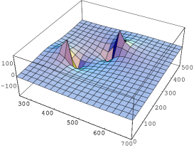
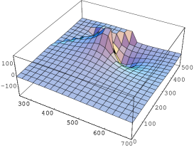
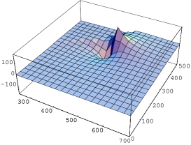
Figure 9: Chiral limit. From left to right, Figs. 9a,b,c respectively. In Fig. 9a the poles of T found in the unphysical sheet are shown for I=0. Analogously for I=1/2 and 1 in Figs. 9b,c respectively.

5 Estimations of the unphysical cut contribution from $\chi$PT and the exchange of resonances.

In this last section we estimate the influence of the unphysical cuts for the elastic $\pi\pi$ and $K\pi$ S-waves with I=0 and 1/2 respectively. The unphysical cuts will be approximated by means of $\chi$PT supplied with the exchange of resonances [24] with spin $\leq$1 in the t- and u-channels. The loops are calculated from $\chi$PT at $\mathcal{O}(p^{4})$ and the exchange of resonances in the crossed channels accounts for a resummation of counterterms up to an infinite order, in the way explained in section 2 after eq. (26). The result can be taken directly from ref. [23], where the $\pi\pi\rightarrow\pi\pi$ and $K\pi\rightarrow K\pi$ amplitudes are calculated up to one loop including explicit resonance fields [24].

In order to extract, from ref. [23], the contribution of the unphysical cuts, which we design by $\hbox{T}_{Left}$, we have made use of eqs. (3.2), (3.10), (3.13), (3.14) for the $\pi\pi$ scattering and of eqs. (3.6), (3.16), (3.19) and (3.20) for the $K\pi$ one. We calculate the loop contributions at the same regularization scale than in [23], that is, $\mu=M_{\rho}=770$ MeV, the same we have taken in this work. In the following, when we refer to an equation in the form (m.n), it should be understood that this equation is the corresponding one from ref. [23]. The work of [23] contains loops and the exchange of resonances in the $s$, $t$ and $u$ channels. The exchange of resonances in the s-channel is also present in our work where the masses and couplings of the scalar resonances, eqs. (79), were fitted to data. Obviously the loops and the exchange of resonances in crossed channels, absent in our work, go to $\hbox{T}_{Left}$. On the other hand, we must also include in $\hbox{T}_{Left}$ a polynomial contribution of $\mathcal{O}(p^{4})$ because the loop functions used in [23], $J_{PQ}^{r}$, $M_{PQ}^{r}$ and $\bar{J}_{PQ}$, where $P$, $Q$ are $\pi$, $K$ or $\eta$, and our loop functions, $(-)g_{0}(s)$, differ in a constant. This polynomial contributions can be interpreted as subtraction terms from a dispersion relation of $\hbox{T}_{Left}$. Since the loops are calculated with ImT at $\mathcal{O}(p^{4})$ one needs three subtractions, which fix the order of the subtraction polynomial. Let us explain first the $\pi\pi$ scattering.

From eq. (3.2) one has the expression of the elastic $\pi\pi$ amplitude with I=0 in terms of the amplitude A$(s,t,u)$, eq. (3.10). Making use of eqs. (3.2) and (3.13) the contribution of the loops in the s-channel is given by

$$\frac{(2s-m_{\pi}^{2})^{2}}{2f_{\pi}^{4}}J^{r}_{\pi\pi}(s)+\frac{3s^{2}}{8f_{\pi}^{4}}J^{r}_{KK}(s)+\frac{m_{\pi}^{4}}{6f_{\pi}^{4}}J^{r}_{\eta\eta}(s)$$ (83)

It is straightforward to see that the imaginary part of eq. (83) is the one required by unitarity up to $\mathcal{O}(p^{4})$ for the I=0 S-wave $\pi\pi$ elastic partial wave with pions, kaons and etas as intermediate states. The squared amplitudes in front of the loop functions are the lowest order $\chi$PT amplitudes since loops are calculated at $\mathcal{O}(p^{4})$. This is the same kind of result we would obtain for the loop contributions in the s-channel from the expansion of the generalization of eq. (45) to coupled channels up to the order considered in eq. (83), after dividing eq. (83) by a global factor 2 to match with our normalization in eq. (1) with $\alpha=2$. However, as we discussed above we use $(-)g_{0}(s)_{ii}$ instead of $J^{r}_{ii}(s)$ in eq. (83) in order to evaluate the loop contributions in the s-channel. Hence, we must include in $\hbox{T}_{Left}$ the following expression

$$\frac{(2s-m_{\pi}^{2})^{2}}{2f_{\pi}^{4}}(J^{r}_{\pi\pi}(s)+g_{0}(s)_{11})+\frac{3s^{2}}{8f_{\pi}^{4}}(J^{r}_{KK}(s)+g_{0}(s)_{22})+\frac{m_{\pi}^{4}}{6f_{\pi}^{4}}(J^{r}_{\eta\eta}(s)+g_{0}(s)_{33})$$ (84)

The former contribution, together with the exchange of resonances and loops in the crossed channels, after projecting over the S-wave using eq. (1) with $\alpha=2$, define $\hbox{T}_{Left}$ in our approach.

For the I=1/2, $L$=0 $K\pi$ partial wave one has essentially the same situation than for $\pi\pi$. From eqs.(3.6) and (3.19) one calculates the contribution of loops, which we project over the S-wave. The loops in the s-channel give the corresponding result to eq. (83) for the $K\pi$ I=1/2 S-wave. In this case, instead of having the loop function $J^{r}_{PP}(s)$, one can write it in terms of $\bar{J}_{K\pi}(s)$ and $\bar{J}_{K\eta}(s)$. After taking into account the difference between $\bar{J}_{PQ}(s)$ and our loop functions, one obtains the analog result to eq. (84) for $K\pi$. This contribution, together with the projection over the S-wave of loops and the exchange of resonances (eqs. (3.6), (3.20)) in crossed channels, give $\hbox{T}_{Left}$.

We have not considered the tadpole contributions coming from pseudoscalar loops without flux of energy and the coupling of scalar resonances to the vacuum ( Fig. 2.b of [23]) because they are reabsorbed into the residues and positions of the CDD poles and the subtraction constant $a_{0}$, eq.(2), which we have phenomenologically fixed.

Table 3: Influence of the unpysical cuts for the I, $L$=0 $\pi\pi$ and I=1/2, $L$=0 $K\pi$ partial waves. The three first columns refer to $\pi\pi$ and the last three to $K\pi$.

$\sqrt{s}$	$\frac{\hbox{T}_{Left}}{|\hbox{T}_{0,11}|}$	$\frac{\hbox{T}_{Left}}{\hbox{T}^{\infty}_{0,11}}$	$\sqrt{s}$	$\frac{\hbox{T}_{Left}}{|\hbox{T}_{0,11}|}$	$\frac{\hbox{T}_{Left}}{\hbox{T}^{\infty}_{0,11}}$
MeV	$\%$	$\%$	MeV	$\%$	$\%$
276	3.7	4.8	634	7.1	8.7
376.	3.5	5.1	684	3.7	4.7
476	4.1	5.7	734	0.3	0.4
576	5.7	6.	784	-2.5	-3.3
676	8.1	6.1	834	-5.7	-7.2
776	11.2	5.6

Including explicit resonance fields as done in [23] increases the range of safe applicability of Chiral Symmetry from $\sqrt{s}\approx$400 MeV, accomplished in $\chi$PT, up to $\sqrt{s}\approx 700-800$ MeV, as can be seen in [23] when comparing their results with the experimental data.

The results which we obtain for the contribution of $\hbox{T}_{Left}$ in the range of energies of [23] are shown in Table 3. In the second and fifth columns we show, respectively, the ratio between $\hbox{T}_{Left}$ and the absolute value of our calculated I, $L$=0 $\pi\pi$ and I=1/2, $L$=0 $K\pi$ partial wave amplitudes up to $\sqrt{s}\approx 800$ MeV. In Table 3 we also compare $\hbox{T}_{Left}$ with the tree level amplitudes $\hbox{T}^{\infty}_{0,11}$. This ratio is also significative because the procedure which we have followed to arrive to a unitarized amplitude from $\hbox{T}^{\infty}_{0,11}$ would not be much affected by the addition of $\hbox{T}_{Left}$ which is a small correction with respect to $\hbox{T}^{\infty}_{0,11}$. We see that these ratios are rather small. Therefore, this supports our point of view of treating the left hand cut as a perturbation in the range of energies we have considered.

It is worth mentioning that this smallness of the unphysical cuts, as shown in Table 3, is a consequence of a cancellation between the contributions to T_Left from the loops and the exchange of resonances in crossed channels. In fact, the individual contributions in the $\pi\pi$ case, for energies around $\sqrt{s}=600$ MeV, are of the order of 15-20$\%$ with respect to $\hbox{T}^{\infty}_{0,11}$.

In a recent work, ref. [57], the authors also combine the N/D method with chiral symmetry studying the (I,$L$)=(0,0), (2,0) and (1,1) $\pi\pi$ partial wave amplitudes. However, in this work only elastic unitarity is considered and the calculations are done in the chiral limit ($m_{\pi}=0$). On the other hand, the left hand cut is approximated only by the exchange of the $\rho$ plus a scalar resonance without including loops in the crossed channels. These loops, as we have seen in this section, cancel to a large extend the crossed resonance contributions for the S-wave I=0 $\pi\pi$ scattering.

6 Conclusions

Making use of the $N/D$ method, we have developed the most general structure that an elastic partial wave amplitude has when the unphysical cuts are neglected. After matching this result with lowest order, ${\mathcal{O}}(p^{2})$, $\chi PT$ [16] and with the exchange of resonances with spin $\leq$1, in a way consistent with chiral symmetry as given in ref. [24], we extend the formalism to handle also coupled channels. Then, $\pi\pi$ and $K\pi$(I=1/2) P-wave amplitudes are described up to $\sqrt{s}=1.2$ GeV. It is shown that these amplitudes can be given rather accurately in terms of $m_{\pi}$, $m_{K}$, $f$ and the masses of the $\rho$ and $K^{*}$ resonances, when restrictions coming from Large $N_{c}$ QCD and unitarity are considered, in the lines of what was observed in [4].

Next, the scalar sector is studied and good agreement with experiment up to $\sqrt{s}=1.4$ GeV is found. An octet and a singlet are included with masses around 1.4 and 1 GeV respectively. The former originates the observed $f_{0}(1500)$, $a_{0}(1450)$ and $K^{*}_{0}(1430)$ resonances, the latter an important contribution to the physical pole of the $f_{0}(980)$. Other poles appearing in our amplitudes, the $a_{0}(980)$, $\sigma$, $\kappa$ and an important contribution to the final $f_{0}(980)$, originate from meson-meson scattering with the lowest order $\chi PT$ amplitudes plus the constant $a^{SL}$ as dynamics source. This situation is very different from the one observed in the vector channels where tree level structures dominate the scattering process and a strong suppression of unitarity loops occurs, as indicated at the end of section 4. As a consequence, the present study supports that a concept like scalar meson dominance, analogous to the well known vector meson one, is not suited at the phenomenological level.

In the last section we have made some estimations in order to investigate the influence of the unphysical cuts. The results obtained support our picture of treating the unphysical cuts in a perturbative way and then establishing the stability of our conclusions in sections 3 and 4 against the corrections coming from cross symmetry.

Acknowledgments

We would like to acknowledge fruitful and basic discussions for the present work with A. Pich. Discussions with S. Peris, J.R. Peláez and A. Kataev are also acknowledged. This work was partially supported by DGICYT under contacts PB96-0753 and by the EEC-TMR Program$-$Contact No. ERBFMRX-CT98-0169. J. A. O. acknowledges financial support from the Generalitat Valenciana.

Appendix A N/D in coupled channels

In this appendix we make use of a matrix formalism to deal with several coupled channels. In analogy with the elastic case, eq. (7), let us define the matrix $\hbox{T}^{\prime}_{L}$ as

$$\hbox{T}^{\prime}_{L}(s)=p^{-L}\hbox{T}_{L}(s)p^{-L}$$ (85)

with $p$ a diagonal matrix which elements are $p_{ij}=p_{i}\delta_{ij}$ where $p_{i}$ is the modulus of the CM momentum of the channel $i$, $\displaystyle{p_{i}=\frac{\lambda^{1/2}(s,m_{1i}^{2},m_{2i}^{2})}{2\sqrt{s}}}$, with $m_{1i}$ and $m_{2i}$ the masses of the two mesons in channel $i$.

From the beginning we neglect the unphysical cuts. As a consequence $\hbox{T}_{L}(s)_{ij}$ will be proportional to $p_{i}^{L}p_{j}^{L}$. This makes that $\hbox{T}_{L}(s)_{ij}$, apart from the right hand cut coming from unitarity (above the thresholds for channels $i$ and $j$, $s_{th}^{i}$ and $s_{th}^{j}$ respectively), will have another cut for odd $L$ between $s_{th}^{i}$ and $s_{th}^{j}$ due to the square roots present in $p_{i}$ and $p_{j}$. In this way, $\hbox{T}^{\prime}_{L}$ will be free of this cut and will have only the right hand cut coming from unitarity. Thus it will satisfy

$$\hbox{Im T}^{\prime-1}_{L}(s)=-p^{L}\rho(s)p^{L}=-\rho(s)p^{2L}$$ (86)

where $\rho(s)$ is a diagonal matrix defined by

$$\rho(s)=-\frac{p}{8\pi\sqrt{s}}\theta(s)$$ (87)

with $\theta(s)$ another diagonal matrix such that $\theta(s)_{ii}$=1 above the threshold of channel $i$ and 0 below it.

We write $\hbox{T}^{\prime}_{L}$ as a quotient of two matrices, $\hbox{N}_{L}$ and $\hbox{D}_{L}$ making use of the coupled channel version of the N/D method [29]

$$\hbox{T}^{\prime}_{L}=\hbox{D}^{\prime-1}_{L}\hbox{N}^{\prime}_{L}$$ (88)

We can always take $\hbox{N}^{\prime}_{L}$ free of poles and also containing all the zeros of $\hbox{T}^{\prime}_{L}$. In such a case $\hbox{N}^{\prime}_{L}$ will be just a matrix of polynomials, we then write

$$\hbox{N}^{\prime}_{L}=\hbox{Q}_{n-L-1}$$ (89)

with $\hbox{Q}_{n-L-1}$ a matrix of polynomials of maximum degree $n-L-1$.

In this way, from eq. (86) and (88) one has

$$\hbox{Im D}^{\prime}_{L}(s)=-\hbox{N}^{\prime}_{L}(s)\rho(s)p^{2L}$$ (90)

and making a dispersion relation for $\hbox{D}^{\prime}_{L}$ one has

$$\hbox{D}^{\prime}_{L}(s)=-\frac{(s-s_{0})^{n}}{\pi}\int_{0}^{\infty}ds^{\prime}\frac{\hbox{Q}_{n-L-1}(s^{\prime})\rho(s^{\prime})p^{2L}(s^{\prime})}{(s^{\prime}-s)(s^{\prime}-s_{0})^{n}}+\hbox{P}_{n-1}$$ (91)

with $\hbox{P}_{n-1}$ a matrix of polynomials of maximum degree $n-1$.

Because $\hbox{N}^{\prime}_{L}$ is just a matrix of polynomials, it can be reabsorbed in $\hbox{D}^{\prime}_{L}$ to give rise to a new $\widetilde{\hbox{D}}^{\prime}_{L}$ which will fulfill eq. (90) but with $\widetilde{\hbox{N}}^{\prime}_{L}=1$. In this way

$$\hbox{T}^{\prime}_{L} = \widetilde{\hbox{D}}^{\prime-1}_{L}$$

$$\widetilde{\hbox{N}}^{\prime}_{L} = 1$$

$$\widetilde{\hbox{D}}_{L}^{\prime} = -\frac{(s-s_{0})^{L}+1}{\pi}\int_{0}^{\infty}\frac{\rho(s^{\prime})p^{2L}(s^{\prime})}{(s^{\prime}-s)(s^{\prime}-s_{0})^{L+1}}+\hbox{R}(s)$$ (92)

with $\hbox{R}(s)$ a matrix of rational functions whose poles will contain the zeros of $\hbox{T}^{\prime}_{L}$. This fact is in clear analogy with the role played by the CDD poles included in Section 2 for the elastic case.

References

• [1] K.L. Au, D. Morgan and M.R. Pennington, Phys. Rev. D 35 (1987) 1633.
• [2] N.A. Tornqvist, Phys. Rev. Lett. 49 (1982) 624; M. Roos and N.A. Tornqvist, Phys. Rev. Lett. 76 (1996) 1575.
• [3] N.N. Achasov and G.N. Shestakov, Phys. Rev. D 49 (1994) 5779.
• [4] F. Guerrero and A. Pich, Phys. Lett. B 412 (1997) 382.
• [5] For general reviews about the issue: L. Montanet, Rep. Prog. Phys. 46 (1983) 337; F. Close, ibid. 51 (1988) 833 and M.R. Pennington, Nucl. Phys. B (Proc. Suppl) 21 (1991) 37.
• [6] D. Morgan, Phys. Lett. B 51 (1974) 71.
• [7] R.J. Jaffe, Phys. Rev. D 15 (1977) 267; R.J. Jaffe, Phys. Rev. D 15 (1977) 281.
• [8] N.N. Achasov, S.A. Devyanin and G.N. Shestakov, Z. Phys. C 22 (1984) 53; N.N. Achasov, S.A. Devyanin and G.N. Shestakov, Phys. Lett. B 96 (1980) 168; N.N. Achasov, S.A. Devyanin and G.N. Shestakov, Phys. Scripta 27 (1983) 330.
• [9] J. Weinstein and N. Isgur, Phys. Rev. Lett. 48 (1982) 659; J. Weinstein and N. Isgur, Phys. Rev. D 27 (1983) 588; J. Weinstein and N. Isgur, Phys. Rev. D 41 (1990) 2236.
• [10] G. Jansen, B.C. Pearce, K. Holinde and J. Speth, Phys. Rev. D 52 (1995) 2690.
• [11] R.L. Jaffe, Phys. Rev. D 15 (1977) 267.
• [12] T. Barnes, in Proceedings of the Fourth Workshop on Polarized Targets Materials and Techniques, Bad Honned, Germany, 1984, edited by W. Meyer (Bonn Univeristy, Bonn, 1984); J.F. Donoghue, in Hadron Spectroscopy-1985, Proceedings of the International Conference, College Park, Maryland, edited by S. Oneda, AIP Conf. Proc. No. 132 (AIP, New York, 1985), p. 460; also, Close [5].
• [13] D. Morgan and M.R. Pennington, Phys. Rev. D 48 (1993) 1185; D. Morgan and M.R. Pennignton, Phys. Lett. B 258 (1991) 444; D. Morgan and M.R. Pennington, Phys. Rev. D 48 (1993) 1185-1204, 5422-5424.
• [14] B.S. Zou and D.V. Bugg, Phys. Rev. D 48 (1993)R3948.
• [15] S. Weinberg, Physica A 96 (1979) 327.
• [16] J. Gasser and H. Leutwyler, Ann. Phys. (NY) 158 (1984) 142, J. Gasser and H. Leutwyler, Nucl. Phys. B 250 (1985) 465, 517, 539; A. Pich, Rep. Prog. Phys. 58 (1995) 563; G. Ecker, Prog. Part. Nucl. Phys. 35 (1995) 1; U.G. Meissner, Rep. Prog. Phys. 56 (1993) 903.
• [17] G.F. Chew and S. Mandelstam, Phys. Rev. 119 (1960) 467.
• [18] K. Kawarabayashi and M. Suzuki, Phys. Rev. Lett. 16 (1996) 255; Rizuddin and Fayyazuddin, Phys. Rev. 147 (1966) 1071.
• [19] J.A. Oller and E. Oset, Nucl. Phys. A 620 (1997) 438.
• [20] J.A. Oller, E. Oset and J.R. PelΓ‘ez, Phys. Rev. D 59 (1999) 074001.
• [21] A. Dobado and J.R. PelΓ‘ez, Phys. Rev. D 56 (1997) 4193
• [22] F. Guerrero and J.A. Oller, to be published in Nucl. Phys. B 537 (1999) 459.
• [23] V. Bernard, N. Kaiser and U.G. Meissner, Nucl. Phys. B 364 (1991) 283.
• [24] G. Ecker, J. Gasser, A. Pich and E. de Rafael, Nucl. Phys. B 321 (1989) 311.
• [25] E. Witten, Nucl. Phys. B 160 (1979) 57.
• [26] L. Castillejo, R.H. Dalitz and F.J. Dyson, Phys. Rev. 101 (1956) 453.
• [27] G.F. Chew and S.C. Frautschi, Phys. Rev. 124 (1961) 264.
• [28] M.S. Chanowitz, M. Golden and H. Georgi, Phys. Rev. D 36 (1987) 1490.
• [29] J.D. Bjorken, Phys. Rev. Lett. 4 (1960) 473.
• [30] C. Cason et al., The European Physical Journal C 3(1998)1.
• [31] G. Ecker, J. Gasser, H. Leutwyler, A. Pich and E. de Rafael, Phys. Lett. B 223 (1989) 425.
• [32] S.J. Lindenbaum and R.S. Longacre, Phys. Lett. B 274 (1992) 492.
• [33] P. Estrabooks and A.D. Martin, Nucl. Phys. B 79 (1974) 301.
• [34] R. Mercer et al., Nucl. Phys. B 32 (1971) 381.
• [35] P. Estrabooks et al., Nucl. Phys. B 133 (1978) 490.
• [36] H. Leutwyler, Nucl. Phys. B (Proc. Suppl.) 7A (1989) 42.
• [37] T.N. Truong, Phys. Rev. Lett. 61 (1988) 2526; ibid. 67 (1991) 2260; A. Dobado, M.J. Herrero and T.N. Truong, Phys. Lett. B 235 (1990) 134; A. Dobado and J.R. PelΓ‘ez, Phys. Rev. D 47 (1993) 4883; J.A. Oller, E. Oset and J.R. PelΓ‘ez, Phys. Rev. Lett. 80 (1998) 3452.
• [38] A. Dobado and J.R. PelΓ‘ez, Phys. Rev. D 56 (1997) 3057; J.A. Oller and F. Guerrero, Nucl.Phys. B 537 (1999) 459.
• [39] A. Dobado, M.J. Herrero and T.N. Truong, Phys. Lett. B 235 (1990) 129; A. Dobado, M.J. Herrero and J. TerrΓ³n, Z. Phys. C 50 (1991) 205; Z. Phys. C 50 (1991) 465; J.R. PelΓ‘ez, Phys. Rev. D 55 (1997) 4193.
• [40] See J. Gasser and H. Leutwyler in [16] corresponding to year 1985.
• [41] H. Leutwyler and M. Roos, Z. Phys. C 25 (1984) 91.
• [42] T.A. Armstrong et al., Z. Phys. C 52 (1991) 389.
• [43] B. Hyams et al., Nucl. Phys. B 64 (1973) 134; P. Estrabooks et al., AIP Conf. Proc. 13 (1973) 37; G. Grayer et al., Proc. 3rd Philadelphia Conf. on Experimental Meson Spectroscopy, Philadelphia, 1972 (American Institute of Physics, New York, 1972) 5; S.D. Protopopescu and M. Alson-Garnjost, Phys. Rev. D 7 (1973) 1279.
• [44] R. Kaminski, L. Lesniak and K. Rybicki, Z. Phys. C 74 (1997) 79.
• [45] W. Ochs, University of Munich, thesis, 1974.
• [46] C.D. Frogratt and J.L. Petersen, Nucl. Phys. B 129 (1977) 89.
• [47] D. Cohen et al., Phys. Rev. D 22 (1980) 2595.
• [48] A. Etkin et al., Phys. Rev. D 28 (1982) 1786.
• [49] W. Wetzel et al., Nucl. Phys. B 115 (1976) 208; V.A. Polychronakos et al., Phys. Rev. D 19 (1979) 1317; G. Costa et al., Nucl. Phys. B 175 (1980) 402.
• [50] D. Aston et al., Nucl. Phys. B 296 (1988) 493.
• [51] H.H. Bingham et al., Nucl. Phys. B 41 (1972) 1.
• [52] Amsterdam-CERN-Nijmegen-Oxford Collaboration, Phys. Lett. B 63 (1976) 220.
• [53] S. Peris, M. Perrottet and E. de Rafael, J. High Energy Physics 05 (1998) 011.
• [54] A. A. Andrianov, D. Espriu and R. Tarrach, Nucl.Phys. B 533 (1998) 429.
• [55] L. Rosselet et al., Phys. Rev. D 15 (1997) 574.
• [56] A. Schenk, Nucl. Phys. B 363 (1991) 97.
• [57] K. Igi and K. Hikasa, Phys Rev. D 59 (1999) 034005.