Production of
Supersymmetric Particles
at High-Energy Colliders
Dissertation
zur Erlangung des Doktorgrades
des Fachbereichs Physik
der Universität Hamburg
vorgelegt von
Tilman Plehn
aus Siegen
Hamburg
1998

Gutachter der Dissertation: Prof. Dr. P.M. Zerwas Prof. Dr. J. Bartels Gutachter der Disputation: Prof. Dr. P.M. Zerwas Prof. Dr. G. Kramer Datum der Disputation: 13. Juli 1998 Sprecher des Fachbereichs Physik und Vorsitzender des Promotionsausschusses: Prof. Dr. B. Kramer

Abstract

The production and decay of supersymmetric particles is presented in this thesis. The search for light mixing top squarks and neutralinos/charginos will be a major task at the upgraded Tevatron and the LHC as well as at a future $e^{+}e^{-}$ linear collider. The dependence of the hadro-production cross section for weakly and strongly interacting particles on the renormalization and factorization scales is found to be weak in next-to-leading order supersymmetric QCD. This yields an improvement of derived mass bounds or the measurement of the masses, respectively, of neutralinos/charginos and stops at the Tevatron and at the LHC. Moreover, the next-to-leading order corrections increase the predicted neutralino/chargino cross section by +20$\%$ to +40$\%$, nearly independent of the mass of the particles. The consistent treatment as well as the phenomenological implications of scalar top mixing are presented. The corrections to strong and weak coupling induced decays of stops, gluinos, and heavy neutralinos [including mixing stop particles] are strongly dependent on the parameters chosen. The decay widths are defined in a renormalization scheme for the mixing angle, which maintains the symmetry between the two stop states to all orders. The correction to the stop production cross sections, depending on the fraction of incoming quarks and gluons, varies between –10$\%$ to +40$\%$ for an increasing fraction of incoming gluons. The dependence of the cross section on all parameters, except for the masses of the produced particles, is in contrast to the light-flavor squark case negligible. The calculation of the stop production cross section was applicable to the Tevatron search for particles which could be responsible for the HERA anomaly.

Zusammenfassung

In dieser Arbeit wird die Produktion und der Zerfall supersymmetrischer Teilchen betrachtet. Die Suche nach leichten mischenden top–Squarks und Neutralinos/Charginos ist eine der wichtigsten Aufgaben am Tevatron und LHC ebenso wie an einem zukünftigen $e^{+}e^{-}$–Linearbeschleuniger. Die Abhängigkeit der Wirkungsquerschnitte für die Produktion stark und schwach koppelnder Teilchen von der Renormierungs– und Faktorisierungsskala ist in nächstführender Ordnung reduziert. Dies erlaubt verbesserte Massenschranken oder eine verbesserte Massenbestimmung für Neutralinos/Charginos und Stops am Tevatron und am LHC. Darüber hinaus vergrößern die Korrekturen den vorhergesagten Wirkungsquerschnitt für Neutralinos/Charginos um +20$\%$ bis +40$\%$, nahezu unabhängig von der Masse der produzierten Teilchen. Weiterhin wird eine konsistente Behandlung der Stop–Mischung vorgestellt und deren phänomenologische Konsequenzen untersucht. Die Korrekturen zu starken und schwachen Zerfällen von top–Squarks, Gluinos und schweren Neutralinos — insofern sie top–Squarks enthalten — hängen signifikant von den gewählten Parametern ab. Die Zerfallsbreiten enthalten die Definition des Stop–Mischungswinkels, welche die Symmetrie zwischen den beiden Stop–Zuständen in beliebiger Ordnung Störungstheorie erhält. Die Korrekturen zu den Wirkungsquerschnitten für Stop–Produktion variieren zwischen –10$\%$ und +40$\%$ und wachsen mit dem Anteil einlaufender Gluonen gegenüber Quarks. Im Gegensatz zur Produktion massenentarteter Squarks ist die Abhängigkeit von Parametern über die Stop–Masse hinaus vernachlässigbar. Die Berechnung des Wirkungsquerschitts für die Stop–Produktion konnte am Tevatron auf die Suche nach Teilchen, die für die HERA–Anomalie verantwortlich sein könnten, angewandt werden.

Vernunft und Wissenschaft gehen oft verschiedene Wege

Paul K. Feyerabend, Wider den Methodenzwang

Introduction

A fundamental element of particle physics are symmetry principles. The electroweak as well as the strong interaction, combined to the Standard Model, are based on the gauge symmetry group SU(3)$\times$SU(2)$\times$U(1). The extension [1] of this concept to a theory incorporating global or local supersymmetry is a well-motivated step for several reasons:

The Standard Model has been well-established by the discovery of the gluon and the weak gauge bosons, and by precision measurements at LEP and at the Tevatron, as well as at HERA. Currently, there is no experimental compulsion to modify the Standard Model at energy scales accessible to these colliders, provided the predicted Higgs boson will be found at LEP or at a future hadron or electron collider. However, a set of conceptual problems cannot be solved in the Standard Model framework: The mass of the only fundamental scalar particle, the Higgs boson, is not stable under quantum fluctuations, i.e. loop contributions to the Higgs mass term become large at high scales and have to be absorbed into the counter terms for the physical Higgs mass. This hierarchy problem leads to fine tuning of the parameters in the Higgs potential, to avoid the breakdown of perturbative weak symmetry breaking.

Possible grand unification scenarios are based on a gauge group at some high unification scale, which contains the different Standard Model gauge groups. Simple unification groups are the SU(5) [2] or SO(10) [3], the latter favored in scenarios with massive neutrinos. Non-minimal scenarios may yield intermediate symmetries and threshold effects, but as long as they include a simple unifying gauge group, the three running Standard Model couplings have to meet in one point at the unification scale. The requirement of one unification point and additional bounds from the non-observation of the proton decay lead to difficulties in the Standard Model, when it is embedded into a grand desert scenario, and most likely restrict the validity of the Standard Model to scales around the weak scale.

In supersymmetric extensions of the Standard Model the masses of scalar particles remain stable even for very large scales, as required by grand unification scenarios. Quantum fluctuations due to fermions and bosons cancel each other; the leading singularities also vanish in softly broken supersymmetric theories. The hierarchy problem does therefore not occur in the extended supersymmetric Higgs sector. Including an intermediate supersymmetry breaking scale, the minimal supersymmetric extension of the Standard Model may be valid up to a grand unification scale without any fine tuning, being compatible with grand desert unification scenarios. Given the strong and the Fermi coupling constant at low scales, it predicts the weak mixing angle in very good agreement with the measured value [4]. For a large top quark mass the renormalization group evolution can drive the electroweak symmetry breaking at low scales. The minimal supersymmetric Higgs sector consists of two doublets, in order to give masses to up and down type quarks while preserving supersymmetry and gauge invariance. Hence, after breaking the weak gauge symmetry, five physical Higgs bosons occur. The non-diagonal CP even current eigenstates yield a light scalar Higgs boson with a strong theoretical upper bound on its mass. In some regimes of the supersymmetric parameter space this particle is accessible to LEP2, and the dependence of the theoretical mass bound on low-energy supersymmetry parameters can be used to constrain the fundamental mixing parameter $\tan\beta$.

In supersymmetric $R$ parity conserving models the lightest supersymmetric particle is stable. This LSP, which in many scenarios turns out to be the lightest neutralino, is a possible candidate for cosmological cold dark matter.

In analogy to the gauge symmetries one may extend the global to a local supersymmetry. This invariance gives rise to higher spin states in the Lagrangean: a massless spin-2 graviton field and its spin-3/2 gravitino partner appear [5]. The general Einstein-gravitation is implemented into a theory of the strong and electroweak interaction. The so-obtained Kähler potential can in simple cases be derived by superstring compactification [6].

The breaking of exact supersymmetry is reflected in the observed mass difference between the Standard Model particles and their partners. Due to the current mass limits, this mass difference is, in case of strongly interacting particles, much larger than the typical mass scale of the Standard Model particles. Assuming no mixing for light-flavor squarks, there are stringent mass limits on the squarks and gluinos from the direct search at the Tevatron [7, 8]. Due to large Yukawa couplings, the partners of the third generation Standard Model particles may mix. Since more parameters of the supersymmetric Lagrangean enter through the non-diagonal mass matrices and the couplings, the mass limits for these third generation sfermions are weakened. Moreover, all supersymmetric partners of the electroweak gauge bosons and the extended Higgs boson degrees of freedom mix. The search for these weakly interacting particles, neutralinos and charginos, at hadron colliders [7] has not reached its limitations and will complete the limits obtained from the search at LEP2 [9]. The search for strongly interacting and also for light weakly interacting supersymmetric particles is one major task for the upgraded Tevatron and the LHC. The investigation of mixing effects in the strong and weak coupling sector requires precision measurements at hadron as well as at lepton colliders.

The reconstruction of supersymmetric particles from detector data is difficult in $R$ parity conserving theories, since two LSPs leave the detector unobserved. Moreover, hadron colliders do not have an incoming partonic state with well-defined kinematics, but the partonic cross sections have to be convoluted with parton density functions. The derivation of mass bounds or the mass determination, respectively, has to be performed by measuring the total hadronic cross section, if rather specific final state cascades cannot be used to determine the mass. Especially for strongly interacting final state particles, the cross sections depend on the factorization and renormalization scales through the parton densities and the running QCD coupling. The scale dependences lead to considerable uncertainties in the determination of mass bounds. The next-to-leading order cross sections will improve the mass bounds not only by their accuracy but also by their size. These hadronic cross sections for mixing supersymmetric particles at the upgraded Tevatron as well as at the LHC will be given in this thesis.

Similarly to light-flavor squarks and gluinos, the search for top squarks with a non-zero mixing angle will lead to stringent mass bounds, which are essentially independent of the mixing parameters and the masses of other supersymmetric particles. However, it will most likely be impossible to measure the mixing angle at hadron colliders directly, since the cross sections for the production of a mixed stop pair are strongly suppressed. The analysis of mixing effects in the stop sector will be completed by the direct measurement of the mixing angle in $e^{+}e^{-}$ collisions [10].

Regarding certain decay channels the direct search for gauginos and higgsinos at hadron colliders resembles the search for weak gauge bosons. Although in most supergravity inspired scenarios not all gauginos and higgsinos are light enough to be found at the upgraded Tevatron, the search for light neutral and charged gauginos is promising and could improve the LEP2 results at the upgraded Tevatron and at the LHC. Even if the leading order cross sections are independent of the QCD coupling, they depend on the factorization scale through the parton densities. The next-to-leading order predictions will again considerably improve the bounds derived for masses and couplings.

However, all search strategies for supersymmetric particles depend on cascade decays leading to leptons, jets, and LSPs in the final state, the latter provided $R$ parity is conserved. As long as the masses of the particles under consideration are not known, the analysis of these multiple decay channels does not give strong limits, e.g. on mixing parameters involved. But for a sufficiently large sample of events including supersymmetric particles, the whole variety of possible decays and couplings will help to determine the mass and mixing parameters of the supersymmetric extension of the Standard Model. The measurement of low energy parameters can then be used to search for universal parameters, predicted by grand unification or supergravity inspired scenarios.

Outline of the Thesis

Since the supersymmetric observables presented in the following analyses can, from a phenomenological point of view, be treated independently, technical features are covered with their first appearance.

The general physics background is described in the first chapter. A short introduction into supersymmetric extensions of the Standard Model is complemented by the discussion of special aspects concerning mixing particles; the next-to-leading order treatment of the mixing angle [11] in the CP conserving stop sector is presented, and the regularization prescriptions used for supersymmetric gauge theories are summarized. The supersymmetric Feynman rules and a complete set of formulae considered useful for the detailed understanding of the calculations are given in the appendices.

The production cross sections for neutralinos and charginos at hadron colliders are treated in chapter 2. They include the virtual and real next-to-leading order corrections, the latter calculated using the dipole subtraction method. The treatment of on-shell singularities is described in detail. The possible improvement of the current analysis by using the next-to-leading order cross section is pointed out.

In chapter 3 the decay widths including mixing stop particles in next-to-leading order supersymmetric QCD [11] are given. They include weak and strong coupling stop decays as well as gluino and heavy neutralino decays to a light stop. The treatment of the mixing angle follows the theoretical description in chapter 1. The complete analytical results for the next-to-leading order stop decay width is presented in the appendix.

The study of scalar top quarks is continued in chapter 4, where the production cross section at hadron colliders is given for both of the mass eigenstates in next-to-leading order supersymmetric QCD [12]. One crucial point is the influence of the mixing angle and supersymmetric parameters, which are present in the virtual corrections, on the experimental analysis and on the mass bounds. The real gluon emission is calculated using the cut-off method.

For a light stop the production cross section at hadron colliders can be adapted to $R$ parity violating scenarios [14]. The resonance cross section for the production of $R$ parity violating squarks in $ep$ collisions is calculated in next-to-leading order [13], and the search results for these particles at HERA and at the Tevatron are combined. The influence of other search strategies for $R$ parity violating squarks is reviewed.

The analytical calculations have been performed using the symbolic manipulation program FORM [15], for the numerical integration routine VEGAS [16] was chosen, and the parton cross sections have been calculated using the CTEQ4 [17] parton densities in leading and next-to-leading order.

Chapter 1 Supersymmetry

1.1 Supersymmetric Extensions of the Standard Model

Global supersymmetry is a possible extension of the set of symmetries appearing in flat space-time gauge theories. The most general extension of a Poincaré invariant theory would be an $N$-extended super-Poincaré Algebra containing central charges [18, 1]. The supersymmetry generators $Q^{i}\;[i=1,...,N]$ and their complex conjugate $\overline{Q}^{i}$ transform fermionic into bosonic fields and vice versa, therefore obeying an anticommutation relation. These anticommutators lead to a ${\mathbb{Z}}_{2}$ graded Lie algebra, containing the supersymmetry as well as the Poincaré group generators and circumventing the No-Go theorem [19]. The dimension of the extension $N$ determines the maximum spin present in the particle spectrum of the theory. Renormalizability requires a maximum spin of one for global supersymmetry, which is equivalent to $N\leq 4$. Including the graviton results a maximum spin two for local supersymmetry, supergravity, and renders $N\leq 8$. For $N=1$ this super-Poincaré algebra becomes particularly simple, since the central charges vanish and the generators $Q,\overline{Q}$ anticommute with themselves. Extended supersymmetric theories have some remarkable features: for $N=2$ the particle spectrum can be calculated non-perturbatively [20], $N=4$ leads to a completely finite theory, and $N\geq 5$ contains gravitation. However, the observed low energy particle spectrum and CP violation are only compatible with ($N$=1) global supersymmetry. We will make use of the incorporation of global supersymmetry into local supergravity only by assuming certain characteristics of the mass spectrum at high scales, where unification is required.

Since supersymmetric theories by definition contain scalar particles not only in the Higgs sector, the behavior of scalar masses is of importance: In the Standard Model the scalar Higgs boson mass suffers from UV divergent radiative corrections, proportional to $g^{2}\Lambda^{2}$ where $g$ is a gauge coupling and $\Lambda$ is an UV cut-off parameter. This cut-off parameter could be fixed by some scale where new physics appears. Assuming the Standard Model not being an effective theory for mass scales around the weak gauge boson mass, e.g. leads to a physical scalar mass of the order of the weak scale and higher order loop contributions of the order of the cut-off, which could be the Planck scale. These corrections have to be absorbed, using fine-tuning of mass and coupling counter terms in the Lagrangean. The large corrections in the Standard Model originate from gauge boson and top quark loops. In supersymmetric extensions additional corrections arising from the supersymmetric partners enter with a minus sign and weaken the UV degree of divergence to a logarithmic behavior [$\delta m/m\propto\log\Lambda^{2}$]. For broken supersymmetry another term proportional to the mass difference between the Standard Model loop particles and their supersymmetric partners arises. Assuming e.g. a grand desert SU(5) scenario the natural shift of the scalar masses between the weak and the unification scale is limited to less than one order of magnitude [22].

Assuming a supersymmetric extension of the Standard Model, the evolution of the gauge couplings can be evaluated, based on different scenarios. Embedding the Standard Model into a simple GUT gauge group does neither fix the gauge group nor possible intermediate scenarios, i.e. SU(5) unification with a grand desert is only one possibility. The evolution of the gauge couplings depends on threshold effects and masses in intermediate unification models. However, it can be shown, that, using supersymmetry, the gauge couplings unify up to a certain accuracy, Fig. 1.1. The unification of the three Standard Model gauge couplings determines one of the three parameters involved [$\alpha,s_{w}^{2}\equiv\sin^{2}\theta_{w},\alpha_{s}$] theoretically. This prediction has to be compared to the measured value e.g. for the weak mixing angle in the $\overline{{\rm MS}}$ scheme. In contrast to the Standard Model, which for reasons described above will hardly be valid up to a large unification scale, the predicted value for the minimal supersymmetric extension of the Standard Model $s^{2}_{w}(m_{\scriptscriptstyle Z})=0.2334\pm 0.005$ agrees very well with the measured value of $0.2316\pm 0.0003$ [4]. Any specific GUT scenario fixes the renormalization group evolution of all the masses and couplings. The determination of $\alpha_{s}(m_{\scriptscriptstyle Z})$ from $\alpha$ and $s^{2}_{w}$ again reflects the improvement of the Standard Model one-scale GUT, which gives $\alpha_{s}(m_{\scriptscriptstyle Z})=0.073\pm 0.002$, to the supersymmetric one-scale GUT, which yields $\alpha_{s}(m_{\scriptscriptstyle Z})=0.129\pm 0.010$. However, the measured value of $\alpha_{s}(m_{\scriptscriptstyle Z})=0.118\pm 0.004$ indicates, that the minimal supersymmetric GUT prefers a slightly larger value; threshold effects may be responsible for the difference. Very light gauginos and very heavy squarks might even for the SU(5) GUT model lead to the measured value of $\alpha_{s}$ [22].

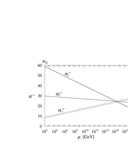
Figure 1.1: The renormalization group evolution of the three Standard Model gauge couplings, assuming a simple SU(5) GUT gauge group and a grand desert [22].

1.2 The Minimal Supersymmetric Standard Model

The Minimal Supersymmetric Standard Model [MSSM] adds a minimal set of supersymmetric partner fields to the Standard Model [SM]. These fields contain scalar partners – sleptons and squarks – of all chiral eigenstates of the Dirac fermions, incorporated into chiral supermultiplets. Absorbing Standard Model gauge fields into vector supermultiplets leaves Majorana fermion partners of the neutral U(1), SU(2), SU(3) gauge fields and Dirac fermion partners of the charged SU(2) gauge fields, called gauginos. The SU(3) ghost fields are defined by re-writing the Fadeev-Popov determinant; therefore they do not receive supersymmetric partners, which enter by requiring the original Lagrangean being invariant under a global supersymmetry transformation.

For reasons described later in this chapter the supersymmetric scalar potential cannot include conjugate fields. Hence, at least two different complex Higgs doublets have to be introduced to give masses to up and down type quarks. They form five physical Higgs particles after breaking SU(2)$\times$U(1) invariance. This extension of the Higgs sector is not generically supersymmetric. However these scalar Higgs degrees of freedom have to develop partner fields. This yields neutral and charged Majorana/Dirac fermions with the same quantum numbers as the SU(2) gauginos.

The supersymmetric Lagrangean in superspace can be constructed by extending the integration over the Lagrange density from space-time to a superspace integration, i.e. by adding two Grassmann dimensions $\{\theta,\bar{\theta}\}$. All superfields can be written as a finite power series in these Grassmann variables, containing the component fields in the coefficients. Only two elements enter the supersymmetric Lagrangean: (i) the so-called $F$ term of a chiral supermultiplet, denoted as $\Phi_{\theta^{2}}$ in the expansion of the superfield in the Grassmann variable $\theta$; (ii) the $D$ term of a vector multiplet $V_{\theta^{2}\bar{\theta}^{2}}$ [1]. The kinetic real vector supermultiplet is defined as the product of a chiral supermultiplet and its conjugate $\overline{\Phi}_{j}\Phi_{j}$, its $D$ terms contain the $F$ components of the chiral multiplets $F_{j}^{*}F_{j}$, which is absorbed into the scalar potential.

The most general ansatz for a superpotential formed by chiral supermultiplets relies on the fact, that the product of two chiral supermultiplet is again chiral:

$${\cal W}(\{\Phi\})=m_{ij}\Phi_{i}\Phi_{j}+\lambda_{ijk}\Phi_{i}\Phi_{j}\Phi_{k}$$ (1.1)

Higher orders in the polynomial would give mass dimensions bigger than four and therefore spoil renormalizability. The superpotential occurs in the Lagrangean as (${\cal W}+\overline{{\cal W}}$). The scalar potential in the component-field Lagrangean contains, after integration over the Grassmann variables, the non-Yukawa terms arising from the superpotential ${\cal W}$; it is defined as

$${\cal V}=-\left(F_{j}^{*}F_{j}+\frac{\partial{\cal W}(A)}{\partial A_{j}}F_{j}+\frac{\partial\overline{{\cal W}}(\overline{A})}{\partial\overline{A}_{j}}F_{j}^{*}\right)$$ (1.2)

The Euler-Lagrange equations yield $F_{j}^{*}=-\partial{\cal W}(A)/\partial A_{j}$ where $A_{j}$ are the sfermion fields in the supermultiplet. This fixes the most general scalar potential including chiral supermultiplets in the matter sector of the Lagrangean:

$${\cal V}=\sum_{j}\left|F_{j}\right|^{2}$$ (1.3)

Including the gauge sector for a non-abelian gauge group leads to vector multiplets containing the gauge fields and their partners. The scalar potential will also contain the $D$ auxiliary component field terms of the gauge multiplet

$${\cal V}=\sum_{j}\left|F_{j}\right|^{2}+\frac{1}{2}\sum_{a}\left(D^{a}\right)^{2}=\sum_{j}\left|F_{j}\right|^{2}+\frac{g^{2}}{2}\sum_{a}\left(S^{*}T^{a}S\right)^{2}$$ (1.4)

The $D$ term is written for a general non-abelian SU(N) gauge group. $S$ are the scalar fields transforming under the fundamental representation of the corresponding gauge group, and $T^{a}$ the generators of the underlying gauge group.

1.2.1 $\mathbf{R}$ Parity

The most general superpotential as given in eq.(1.1) contains trilinear couplings of chiral matter supermultiplets, like the Higgs, the quark, and the lepton supermultiplet. Couplings between the different Higgs fields or between the Higgs field and corresponding lepton or quark supermultiplets are needed to construct the two doublet Higgs sector in the scalar potential. Although these vertices conserve the over-all fermion number, they may violate the baryon and lepton number and would lead to the same effects as leptoquarks, e.g. proton decay [23]. In extensions of the Standard Model these operators are forbidden by gauge invariance, as long as their dimension is less than six. The MSSM either needs to suppress the different couplings or remove the whole set by applying a new ${\mathbb{Z}}_{2}$ symmetry which changes the sign of the Grassmann variables in the Lagrangean. The corresponding conserved charge is defined as

$$R=(-1)^{3B+L+2S}$$ (1.5)

where $B$ is the baryon number, $L$ the lepton number, and $S$ the spin of the particle. This number is chosen to give $(+)$ for Standard Model particles and $(-)$ for supersymmetric partners. The Higgs particles in the two doublet model are all described by $R=+1$. Accounting for $R$ symmetry in the supersymmetric Lagrangean removes trilinear chiral supermultiplet vertices containing no Higgs superfield. The general superpotential eq.(1.1) can be separated into an $R$ parity conserving and an $R$ parity violating part, which read for one generation of quarks and leptons

$${\cal W}= \;{\cal W}_{R}+{\cal W}_{\hbox to0.0pt{\hbox{$\mskip 1.0mu/$}\hss}R}$$

$${\cal W}_{R}= \;\lambda^{E}\overline{E}H_{1}^{j}L^{j}+\lambda^{D}\overline{D}H_{1}^{j}Q^{j}+\lambda^{U}\overline{U}H_{2}^{j}Q^{j}-\mu H_{1}^{j}H_{2}^{j}$$

$${\cal W}_{\hbox to0.0pt{\hbox{$\mskip 1.0mu/$}\hss}R}= \;\frac{1}{2}\lambda L^{j}L^{j}\overline{E}+\lambda^{\prime}L^{j}Q^{j}\overline{D}+\frac{1}{2}\lambda^{\prime\prime}\overline{U}\,\overline{D}\,\overline{D}$$ (1.6)

The contraction of two indices is defined by the antisymmetric ($2\times 2$) matrix $\epsilon_{ij}$; $L,Q$ are electron and quark doublet superfields, $E,D,U$ are the singlet superfields for the electron, $d$ and $u$ type quark; $\lambda^{E,D,U}$ are the Yukawa coupling matrices, and $\mu$ is the Higgs mass parameter, which also defines the higgsino mass [see appendix A]. The Yukawa couplings $\lambda,\lambda^{\prime}$ violate lepton number, $\lambda^{\prime\prime}$ violates baryon number.

The combination $(\lambda^{\prime}\cdot\lambda^{\prime\prime})$ leads to proton decay via an $s$ channel $d$ type leptoquark and therefore has to be strongly suppressed. The conservation of $R$ is therefore a sufficient condition for the stability of the proton. However, this symmetry has been introduced ad hoc for weak scale supersymmetry as a less rigid substitute for the conservation of some combination of $B$ and $L$. The exact vanishing of $(\lambda^{\prime}\cdot\lambda^{\prime\prime})$ is not a necessary condition for a stable proton; i.e. if ${\cal W}_{\hbox to0.0pt{\hbox{$\mskip 1.0mu/$}\hss}R}$ is not removed by hand by demanding $R$ symmetry in the supersymmetry Lagrangean, then many different constraints can be imposed on combinations of couplings and masses in the $R$ parity violating sector. The limits from direct production at HERA as well as from rare decays generically determine $\lambda\cdot\lambda/m^{2}$, dependent on the flavor of the squark considered. The same holds for atomic parity violation. The bounds from neutral meson mixing influence $\lambda\cdot\lambda/m$, and the direct searches at hadron colliders and LEP are only sensitive to the mass, except for the analysis of specific decay channels [24, 25].

Phenomenologically, exact $R$ parity conservation leads to the existence of a stable lightest supersymmetric particle (LSP), and allows for the production of supersymmetric particles only in pairs. For cosmological reasons this LSP has to be charge and color neutral, which restricts the choices in the MSSM framework to the lightest neutralino or the sneutrino. In GUT models exact $R$ parity conservation is not necessary to obtain low-energy $R$ parity conservation. For broken $R$ parity the unstable ’LSP’ could therefore be long-living and charged, allowing for charginos, sleptons and even stops, as long as the lifetime is small enough to circumvent the cosmological constraints.

1.2.2 Soft Breaking

If supersymmetry would be exact, the squarks and sleptons were mass degenerate with the Standard Model particles. Since the gauge couplings have to respect supersymmetry in order to cancel the quadratic divergences, breaking supersymmetry means enforcing a mass difference between Standard Model particles and their supersymmetric partners. The mechanism of introducing mass terms by soft breaking [26] at a given scale has to respect gauge symmetry, weak-scale $R$ parity, stability of scalar masses, and experimental bounds e.g. on FCNC. Soft breaking terms can be added to the superpotential eq.(1.1) at any given scale. They exhibit the generic form

$${\cal L}_{\rm soft}=-\left(m_{0}^{2}\right)_{ij}C^{*}_{i}C_{j}-\frac{1}{2}\left[\left(m_{1/2}\right)_{j}\lambda_{j}\lambda_{j}+{\rm h.c.}\right]-\left[\frac{1}{6}A_{ijk}C_{i}C_{j}C_{k}+B\mu H_{1}H_{2}+{\rm h.c.}\right]$$ (1.7)

The component fields involved are generic scalars $C$, Majorana fermions $\lambda$ and the Higgs fields $H_{1},H_{2}$, which are again contracted using $\epsilon_{ij}$. The possible set of parameters consists of:

• Scalar mass matrices $(m_{0}^{2})_{ij}\;[i,j=1,...n]$ for squarks and sleptons with $n$ generations. The diagonal masses can be chosen real, since $({\cal W}+\overline{{\cal W}})$ enters the Lagrangean.

• Three real gaugino masses $(m_{1/2})_{j}\;[j=1,2,3]$.

• 27 complex trilinear couplings $A_{ijk}[i,j,k=1,2,3]$ which conserve the $R$ charge.

• Two masses for the Higgs scalars and a complex Higgs mass parameter $\mu BH_{1}^{j}H_{2}^{j}$.

Evolving soft breaking mass terms by means of the renormalization group equations can lead to breaking of the U(1)$\times$SU(2) symmetry by driving one mass squared negative. This generalization of the Coleman-Weinberg mechanism [27] links the large top Yukawa coupling to electroweak symmetry breaking.

1.2.3 Supersymmetric QCD

Particle Content

The search for directly produced supersymmetric particles at hadron colliders is dominated by strongly interacting final states. In these production processes the quantum corrections in next-to-leading order are expected to be significant. Moreover, the corrections to the production of weakly interacting particles at hadron colliders are dominated by strong coupling effects. Although the parton picture and thereby the incoming state is not affected by the heavy supersymmetric partners of quarks and gluons, a consistent description of virtual particle effects requires the inclusion of these particles.

The supersymmetric extension of the QCD part of the Standard Model is straightforward, since the SU(3) invariance is unbroken. One chiral mass superfield $Q$ contains the left handed quark doublets $(u_{\scriptscriptstyle L},d_{\scriptscriptstyle L})$ and their squark partners $(\tilde{u}_{\scriptscriptstyle L},\tilde{d}_{\scriptscriptstyle L})$. Two more superfields $\overline{U},\overline{D}$ connect the quark singlet fields $(u^{c}_{\scriptscriptstyle R},d^{c}_{\scriptscriptstyle R})$ to their partners $(\tilde{u}^{*}_{\scriptscriptstyle R},\tilde{d}^{*}_{\scriptscriptstyle R})$. The ${\rm SU}(3)_{C}\times{\rm SU}(2)_{L}\times{\rm U}(1)_{Y}$ quantum numbers for quarks and squarks are identical. Whereas the $\tilde{q}_{\scriptscriptstyle L}$ is a SU(3) triplet, the $\tilde{q}_{\scriptscriptstyle R}$ is an anti-triplet and couples with $(-T^{a})$ to the quark and gluino, as can be seen in Fig. A.2. The gluon vector superfield mirrors the gluons to gluinos ($\tilde{g}$), which are real Majorana fermions and therefore carry two degrees of freedom. The number of generations is not restricted by supersymmetry. The CKM matrix for the quarks will in the following be assumed to be the unity matrix. The same holds for the squark CKM matrix, which is not fixed by first principles to be either diagonal or equal to the quark matrix.

The general mass matrix for up-type squarks is given by

$${\cal M}^{2}\! = \!\left(\begin{array}[]{cc}m_{Q}^{2}\!+\!m_{q}^{2}\!+\!\left(\frac{1}{2}-\frac{2}{3}s_{w}^{2}\right)m_{\scriptscriptstyle Z}^{2}\cos(2\beta)&-m_{q}\left(A_{q}+\mu\cot\beta\right)\\ -m_{q}\left(A_{q}+\mu\cot\beta\right)&m_{U}^{2}\!+\!m_{q}^{2}\!+\!\frac{2}{3}s_{w}^{2}m_{\scriptscriptstyle Z}^{2}\cos(2\beta)\end{array}\right)$$ (1.10)

For down type squarks $\cot\beta$ in the off-diagonal element has to be replaced by $\tan\beta$. The entries $m_{\scriptscriptstyle Q},m_{\scriptscriptstyle U},A_{q}$ are the soft breaking masses. In the diagonal elements the quark mass still appears, as in exact supersymmetry. The $m_{\scriptscriptstyle Z}$ contributions arise from the different SU(2) quantum numbers of the scalar partners of left and right-handed quarks. For light-flavor squarks this matrix can be assumed being diagonal, since the chirality flip Yukawa interactions are suppressed. For the top flavor these off-diagonal elements cannot be disregarded. Taking into consideration bottom-tau unification the ratio of the Higgs vacuum expectation values $\tan\beta$ has to be either smaller than $\sim$2.5 or larger than $\sim$40. In the second case, a large value for $\tan\beta$ compensates for the small bottom quark mass and yields a strongly mixing sbottom scenario. The results for the stop mixing may be generalized to the sbottom case.

Neglecting additional mixing from a CKM like matrix, the chiral squark eigenstates are equal to the mass eigenstates for the light flavors. If we furthermore assume the soft breaking mass being dominant and invariant under SU(2), then the light-flavor mass matrix is proportional to the unity matrix, i.e. the masses of the ten light flavor squarks are equal. As long as only strong coupling processes are considered, we will have to deal with ten identical particles. This will not be the case for the scalar top sector as will be shown in section 1.2.4.

1.2.4 Mixing Stop Particles

Diagonalization of Mass Matrices

For scalar top quarks the off-diagonal elements of the squark mass matrix eq.(1.10) are large. Any real symmetric mass matrix of the form

$${\cal M}^{2}=\left(\begin{array}[]{cc}{\cal M}^{2}_{LL}&{\cal M}^{2}_{LR}\\ {\cal M}^{2}_{LR}&{\cal M}^{2}_{RR}\end{array}\right)$$ (1.13)

can be diagonalized by a real orthogonal transformation, i.e. a uniquely defined real rotation matrix. The eigenvalues are

$$m^{2}_{\scriptscriptstyle 12}=\frac{1}{2}\left[{\rm Tr}({\cal M}^{2})\mp\left[{\rm Tr}^{2}({\cal M}^{2})-4{\rm Det}({\cal M}^{2})\right]^{1/2}\right]$$ (1.14)

The cosine of the mixing angle can be chosen positive $-\pi/4<\theta<\pi/4$:

$$\cos(2\theta)=\frac{\left|{\cal M}^{2}_{LL}-{\cal M}^{2}_{RR}\right|}{\sqrt{{\rm Tr}^{2}({\cal M}^{2})-4{\rm Det}({\cal M}^{2})}}\qquad\qquad\sin(2\theta)=\frac{2{\cal M}^{2}_{LR}}{\sqrt{{\rm Tr}^{2}({\cal M}^{2})-4{\rm Det}({\cal M}^{2})}}$$ (1.15)

There is no flat limit from different to equal mass eigenvalues for this diagonalization procedure, since the diagonalized matrix would be proportional to the unity matrix and therefore commute with any rotational matrix.

Stop Mixing

In the scalar top sector the unrenormalized chiral eigenstates are $\tilde{t}_{{\scriptscriptstyle L}0},\tilde{t}_{{\scriptscriptstyle R}0}$. The chirality-flip Yukawa interactions give rise to off-diagonal elements in the mass matrix eq.(1.10) i.e. the bare mass eigenstates $\tilde{t}_{10}$ and $\tilde{t}_{20}$ are obtained by a leading-order rotation, as described above.

$$\left(\begin{array}[]{c}\tilde{t}_{10}\\ \tilde{t}_{20}\end{array}\right)=\left(\begin{array}[]{cc}\cos\tilde{\theta}_{0}&\ \sin\tilde{\theta}_{0}\\ -\sin\tilde{\theta}_{0}&\ \cos\tilde{\theta}_{0}\end{array}\right)\left(\begin{array}[]{c}\tilde{t}_{{\scriptscriptstyle L}0}\\ \tilde{t}_{{\scriptscriptstyle R}0}\end{array}\right)$$ (1.22)

Figure 1.2: Feynman diagrams for the stop self energy in NLO, including mixing in the second and third diagram, the top-gluino loop and the pure squark tadpole.

The mass eigenvalues and the leading-order rotation angle $\tilde{\theta}_{0}$ can be expressed by the elements of the mass matrix. However, SUSY-QCD corrections, involving the stop and gluino besides the usual particles of the Standard Model, modify the stop mass matrix and the stop fields. The Feynman diagrams are given in Fig. 1.2. As described in appendix A, the coupling to a quark and a gluino as well as the coupling between four squarks can switch the chirality state and therefore contribute not only to the diagonal but also to the off-diagonal matrix elements. This gives rise to the renormalization of the masses and of the wave functions [$\tilde{t}_{i0}=Z^{1/2}_{ij}\,\tilde{t}_{j}$]. Any leading-order observables concerning the mixing top squarks are linked by a re-rotation of $\pi/2$, denoted by ${\cal P}_{12}$, eq.(A.2). In next-to-leading order this symmetry is broken by the mixing stop self energy. In order to restore this symmetry in any order perturbation theory, we choose a real wave-function renormalization matrix $Z^{1/2}$, which is defined to split into a real orthogonal matrix ${\cal R}(\delta\tilde{\theta})$ and a diagonal matrix $Z^{1/2}_{{\rm diag}}$, i.e. $Z^{1/2}={\cal R}(\delta\tilde{\theta})\,Z^{1/2}_{{\rm diag}}$. The rotational part can be reinterpreted as a shift in the mixing angle [11, 28], given by $\tilde{\theta}_{0}-\delta\tilde{\theta}\equiv\tilde{\theta}$:

$$\left(\begin{array}[]{c}\tilde{t}_{1}\\ \tilde{t}_{2}\end{array}\right)=\left(\begin{array}[]{cc}Z^{-1/2}_{{\rm diag},\,11}&0\\ 0&Z^{-1/2}_{{\rm diag},\,22}\end{array}\right)\left(\begin{array}[]{cc}\cos\tilde{\theta}&\ \sin\tilde{\theta}\\ -\sin\tilde{\theta}&\ \cos\tilde{\theta}\end{array}\right)\left(\begin{array}[]{c}\tilde{t}_{{\scriptscriptstyle L}0}\\ \tilde{t}_{{\scriptscriptstyle R}0}\end{array}\right)$$ (1.31)

This counterterm for the mixing angle allows the diagonalization of the real part of the inverse stop propagator matrix in any fixed-order perturbation theory.

$${\rm Re}\left[D_{\rm ren}^{-1}(p^{2})\right]= \big{(}Z^{1/2}\big{)}^{T}\,\left[p^{2}\>{\rm\bf 1}-{\cal M}^{2}+{\rm Re}\,\Sigma(p^{2})\right]\,\big{(}Z^{1/2}\big{)}$$

$$= \big{(}Z^{1/2}_{\rm diag}\big{)}^{T}\,\left[p^{2}\>{\rm\bf 1}-{\cal R}(\delta\tilde{\theta})^{-1}\left({\cal M}^{2}+{\rm Re}\,\Sigma(p^{2})\right){\cal R}(\delta\tilde{\theta})\right]\,\big{(}Z^{1/2}_{\rm diag}\big{)}$$

$$= \big{(}Z^{1/2}_{\rm diag}\big{)}\,{\rm Re}\,D_{\rm diag}^{-1}(p^{2})\,\big{(}Z^{1/2}_{\rm diag}\big{)}$$ (1.32)

This holds as long as the real part of the unrenormalized stop self-energy matrix ${\rm Re}\Sigma(p^{2})$ and thereby the whole next-to-leading order mass matrix is symmetric. The mixing angle depends on the scale of the self energy matrix

$$\tan\left(2\delta\tilde{\theta}(p^{2})\right)=\frac{2\,{\rm Re}\,\Sigma_{12}(p^{2})}{m_{\tilde{t}_{\scriptscriptstyle 1}}^{2}-m_{\tilde{t}_{\scriptscriptstyle 2}}^{2}+{\rm Re}\,\Sigma_{22}(p^{2})-{\rm Re}\,\Sigma_{11}(p^{2})}=\frac{2\,{\rm Re}\,\Sigma_{12}(p^{2})}{m_{\tilde{t}_{\scriptscriptstyle 1}}^{2}-m_{\tilde{t}_{\scriptscriptstyle 2}}^{2}}+{\cal O}(g^{2})$$ (1.34)

We fix the renormalization constants by imposing the following two conditions on the renormalized stop propagator matrix: (i) the diagonal elements should approach the form $1/D_{{\rm ren},\,jj}(p^{2})\to p^{2}-m_{\tilde{t}_{\scriptscriptstyle j}}^{2}+im_{\tilde{t}_{\scriptscriptstyle j}}\Gamma_{\tilde{t}_{j}}$ for $p^{2}\to m_{\tilde{t}_{\scriptscriptstyle j}}^{2}$, with $m_{\tilde{t}_{\scriptscriptstyle j}}$ denoting the pole masses; (ii) the renormalized (real) mixing angle $\tilde{\theta}$ is defined by requiring the real part of the off-diagonal elements $D_{{\rm ren},\,12}(p^{2})$ and $D_{{\rm ren},\,21}(p^{2})$ to vanish. The three relevant counter terms for external scalar particles are

$$\delta m_{\tilde{t}_{\scriptscriptstyle j}}^{2}=\,\text{Re\,}\Sigma_{jj}(m_{\tilde{t}_{\scriptscriptstyle j}}^{2})\qquad\delta Z_{jj}=-\,\text{Re\,}\dot{\Sigma}_{jj}(m_{\tilde{t}_{\scriptscriptstyle j}}^{2})\qquad\delta\tilde{\theta}(p^{2})=-\frac{\,\text{Re\,}\Sigma_{12}(p^{2})}{m_{\tilde{t}_{\scriptscriptstyle 2}}^{2}-m_{\tilde{t}_{\scriptscriptstyle 1}}^{2}}$$ (1.35)

Thus, for the fixed scale $p^{2}$ the real particles $\tilde{t}_{1}$ and $\tilde{t}_{2}$ propagate independently of each other and do not oscillate.

The so-obtained (running) mixing angle depends on the renormalization point $Q$, which we will indicate by writing $\tilde{\theta}(Q^{2})$. The appropriate choice of $Q$ depends on the characteristic scale of the observable that is analyzed. The real shift connecting two different values of the renormalization point is given by the renormalization group, leading to a finite shift at next-to-leading order SUSY-QCD

$$\tilde{\theta}(Q_{1}^{2})-\tilde{\theta}(Q_{2}^{2})=\frac{C_{F}\alpha_{s}m_{\tilde{g}}m_{t}\cos(2\tilde{\theta})}{\pi(m_{\tilde{t}_{\scriptscriptstyle 2}}^{2}-m_{\tilde{t}_{\scriptscriptstyle 1}}^{2})}\,{\rm Re}\!\left[\;B(Q_{2};m_{\tilde{g}},m_{t})\!-\!B(Q_{1};m_{\tilde{g}},m_{t})\;\right]$$ (1.36)

This shift is independent of the regularization. In the limit of large scales the difference behaves as $\log(Q^{2}/{Q^{\prime}}^{2})$. A numerical example is presented in Fig 1.3. As a noteworthy consequence of the running-mixing-angle scheme, we mention that some LO symmetries of the Lagrangean are retained in the NLO observables. For instance, if for only one kind of external stop particle one chooses $Q=m_{\tilde{t}}$, the results for the other stop particle can be derived by the simple operation ${\cal P}_{12}$, eq.(A.2), which then also acts on the argument of the mixing angle.

Figure 1.3: The dependence of $\tilde{\theta}(Q^{2})$ on the renormalization scale $Q$. The input mass values are: $m_{1/2}=150{\rm\,GeV}$, $m_{0}=800{\rm\,GeV}$, $A_{0}=200{\rm\,GeV}$, $\mu>0$, for which the leading-order mixing angle is given by $1.24$ rad. The minimum of the correction corresponds to the threshold $Q=m_{\tilde{g}}+m_{t}$ in the scalar integral.

Considering virtual stop states with arbitrary $p^{2}$, the off-diagonal elements of the propagator matrix can be absorbed into a redefinition of the mixing of the stop fields, described by an effective (complex) running mixing angle $\tilde{\theta}_{\rm eff}(p^{2})\equiv\tilde{\theta}_{0}-\delta\tilde{\theta}_{\rm eff}(p^{2})$. This generalization amounts to a diagonalization of the complex symmetric stop propagator matrix $D_{{\rm ren}}$, including the full self-energy $\Sigma(p^{2})$, by a complex orthogonal matrix ${\cal R}(\delta\tilde{\theta}_{\rm eff})$ exactly in analogy to eq.(1.32). The so-defined effective running mixing angle is given by

$$\tilde{\theta}_{\rm eff}(p^{2})=\tilde{\theta}_{0}-\frac{1}{2}\arctan\!\left[\frac{2\Sigma_{12}(p^{2})}{m_{\tilde{t}_{\scriptscriptstyle 1}}^{2}-m_{\tilde{t}_{\scriptscriptstyle 2}}^{2}+\Sigma_{22}(p^{2})-\Sigma_{11}(p^{2})}\right]\stackrel{{\scriptstyle{\rm NLO}}}{{\rightarrow}}\tilde{\theta}(p^{2})+\frac{{\rm Im}\,\Sigma_{12}(p^{2})}{m_{\tilde{t}_{\scriptscriptstyle 2}}^{2}-m_{\tilde{t}_{\scriptscriptstyle 1}}^{2}}$$ (1.37)

The complex argument of the trigonometric functions leads to hyperbolic functions. From this point of view the use of a diagonal Breit–Wigner propagator matrix is straightforward. For instance, in the toy process $t\tilde{g}\to t\tilde{g}$ all NLO stop-mixing contributions to the virtual stop exchange can be absorbed by introducing the effective mixing angle in the LO matrix elements. The argument of this effective mixing angle is given by the virtuality of the stop particles in the $s$ channel. This procedure also applies to multi-scale processes like $q\bar{q}\to t\tilde{t}_{i}\tilde{g}\,$ or $e^{+}e^{-}\to\tilde{t}_{1}\bar{\tilde{t}}_{2}$, where the effective $g\tilde{t}_{1}\tilde{t}_{2}/\gamma\tilde{t}_{1}\tilde{t}_{2}$ couplings become non-zero due to the different scales of the redefined stop fields.

There exist other renormalization schemes for the stop mixing angle, either fixing the scale of the running mixing angle at some appropriate scale or absorbing certain diagrams e.g. contributing to the production process $e^{+}e^{-}\to\tilde{t}_{1}\bar{\tilde{t}}_{2}$ [29]. Any of these schemes can be regarded as a prescription to measure the mixing angle, either in the mixed production at $e^{+}e^{-}$ linear colliders or in decay modes or quantum corrections. The mixed production induced scheme however has the disadvantage of introducing the $Z\tilde{t}_{1}\tilde{t}_{2}$ weak coupling constants into the QCD counter terms. The measured values of the mixing angle can be translated from one scheme into another by comparing the counter terms. In Fig. 1.3 the numerical effect of the finite renormalization can be seen to be small; the same holds for the different renormalization schemes, which are numerically almost equivalent.

When fixing the counter term for the stop mixing angle $\tilde{\theta}$, one can express the angle in terms of the parameters appearing in the mass matrix eq.(1.10). The counter term $\delta(\sin(2\tilde{\theta}))$ can be linked to the counter terms of these parameters:

$$s_{2\tilde{\theta}}= \;\frac{2m_{t}(A_{t}+\mu{\rm cot}\beta)}{m_{\tilde{t}_{\scriptscriptstyle 1}}^{2}-m_{\tilde{t}_{\scriptscriptstyle 2}}^{2}}$$

$$\frac{\delta s_{2\tilde{\theta}}}{s_{2\tilde{\theta}}}= \;-\frac{\delta(m_{\tilde{t}_{\scriptscriptstyle 1}}^{2}-m_{\tilde{t}_{\scriptscriptstyle 2}}^{2})}{m_{\tilde{t}_{\scriptscriptstyle 1}}^{2}-m_{\tilde{t}_{\scriptscriptstyle 2}}^{2}}+\frac{\delta m_{t}}{m_{t}}+\frac{\delta(A_{t}+\mu{\rm cot}\beta)}{A_{t}+\mu{\rm cot}\beta}$$ (1.38)

where $\delta x$ denotes the counter term of the parameter $x$. Since $\mu$ and $\beta$ appear in the scalar potential only in the weakly interacting sector, they will not be renormalized in next-to-leading order SUSY-QCD. However, $\delta A_{t}$ can be calculated from the mass and mixing angle counter terms. This reflects the fact, that the system of observables used in the Feynman rules is non-minimal, i.e. the on-shell scheme for the masses and the running mixing angle determine the renormalization of the couplings $\tilde{t}_{1}\tilde{t}_{2}G^{0}$ and $\tilde{t}_{1}\tilde{t}_{2}A^{0}$, where $A_{t}$ appears explicitly [30].

1.3 GUT inspired Mass Spectrum

Next-to-leading order calculations in the framework of light-flavor SUSY-QCD [8] only incorporate a few free parameters: the Standard Model set and the gluino and the light-flavor squark mass. Including mixing stops and the mixing neutralinos/charginos the number of low-energy parameters becomes large. Hence, for a rough phenomenological analysis we will use a simplifying scenario, which could be a SUSY-GUT scenario, either supergravity [5] or gauge mediation [31] inspired.

SUSY-GUT Scenario

Inspired by the unification of the three Standard Model gauge couplings in supersymmetric GUT models we will assume a relation between these couplings and the gaugino masses. Independent of the actual form of the simple gauge group and the connected GUT scenario, the three Standard Model gauge groups are embedded into, and independent of intermediate scale particles and thresholds, we can assume gauge coupling unification.

$$\frac{M_{1}(Q)}{\alpha_{1}(Q)}=\frac{M_{2}(Q)}{\alpha_{2}(Q)}=\frac{M_{3}(Q)}{\alpha_{3}(Q)}=\frac{m_{1/2}(M_{X})}{\alpha_{\rm GUT}(M_{X})}$$ (1.39)

where $m_{1/2}$ is the mass entry in the scalar potential, defined at the unification scale $M_{X}$. There the three gauge couplings unify to $\alpha_{\rm GUT}\simeq 1/26$. For the masses at the weak scale this leads to [33]

$$m_{\tilde{B}}\simeq \;M_{1}(m_{Z})\simeq 0.4\;m_{1/2}$$

$$m_{\tilde{W}}\simeq \;M_{2}(m_{Z})\simeq 0.8\;m_{1/2}$$

$$m_{\tilde{g}}\simeq \;M_{3}(m_{Z})\sim 2.6\;m_{1/2}$$ (1.40)

However, the gluino mass is strongly dependent on the scale which can lead to a difference of $30\%$ between the pole mass $m_{\tilde{g}}$ and the running mass $M_{3}(M_{3})$ [33]. For the derivation of these mass relations it is only necessary to assume a simple unification gauge group arising at a scale $M_{X}\sim 2\cdot 10^{16}{\rm\,GeV}$. The gaugino mass unification can be tested experimentally at the LHC [32] as well as at a future linear collider [10].

Mass Unification

In a supergravity inspired MSSM [mSUGRA] the scalar masses and the trilinear couplings are assumed to be universal at the unification scale $M_{X}$. In simple supergravity models they depend on the gravitino mass scale $m_{3/2}$ and on the cosmological constant [5]. The universal parameters at the unification scale $M_{X}$ will be refered to as $m_{0}$ and $A_{0}$. The parameter $\mu B$ occuring in the Higgs sector of the scalar potential [section 1.2.2] will be fixed by the choice of $m_{1/2},m_{0},A_{0},\tan\beta$ and the Standard Model parameters, and by the requirement of electroweak symmetry breaking, up to its sign. The light-flavor squark masses can be expressed in terms of the universal scalar and gaugino masses, the other parameters only enter the off-diagonal elements of the mass matrix eq.(1.10) and can be neglected

$$m_{\tilde{q}_{\scriptscriptstyle L}}^{2}\simeq m_{0}^{2}+6.3m_{1/2}^{2}+0.35D\qquad\qquad m_{\tilde{q}_{\scriptscriptstyle R}}^{2}\simeq m_{0}^{2}+5.8m_{1/2}^{2}+0.16D$$ (1.41)

where $D=m_{Z}^{2}\cos(2\beta)<0$. For mSUGRA scenarios a general prediction for the light-flavor squark mass can be given [33]

$$m_{\tilde{q}}\gtrsim 0.85m_{\tilde{g}}$$ (1.42)

Approximate Solution

Figure 1.4: Some relevant masses in the approximate mSUGRA scenario for $A_{0}=300{\rm\,GeV},\tan\beta=4,\mu>0$; $m_{0}$ and $m_{1/2}$ are varied between 50 and $400{\rm\,GeV}$.

The stop masses can be expressed in terms of the top Yukawa coupling $Y_{t}=h_{t}^{2}/(4\pi)$. For small $\tan\beta$ they approximately read

$$m_{\tilde{t}_{\scriptscriptstyle L}}^{2}\simeq \;m_{0}^{2}\left(1-\frac{Y_{t}}{2Y_{t}^{\rm IR}}\right)+m_{1/2}^{2}\left(6.3-\frac{7Y_{t}}{3Y_{t}^{\rm IR}}-\left(\frac{Y_{t}}{Y_{t}^{\rm IR}}\right)^{2}\right)+0.35D$$

$$m_{\tilde{t}_{\scriptscriptstyle R}}^{2}\simeq \;m_{0}^{2}\left(1-\frac{Y_{t}}{Y_{t}^{\rm IR}}\right)+m_{1/2}^{2}\left(5.8-\frac{14Y_{t}}{3Y_{t}^{\rm IR}}-\left(\frac{2Y_{t}}{Y_{t}^{\rm IR}}\right)^{2}\right)+0.16D$$

$$A_{t}\simeq \;\left(1-\frac{Y_{t}}{Y_{t}^{\rm IR}}\right)-2m_{1/2}$$

$$m_{t}= \;\frac{vs_{\beta}}{\sqrt{2}}h_{t}$$ (1.43)

The IR fixed point of the top mass is $Y_{t}^{\rm IR}\simeq 8\alpha_{3}/9$ and $Y_{t}/Y_{t}^{\rm IR}$ varies from 0.75 to 1 dependent on $\tan\beta$, becoming unity for $\tan\beta=1$. In this limit the universal scalar mass does not influence the lighter right handed stop mass. If the doublet soft breaking mass is larger than the right handed soft breaking mass, the $\tilde{t}_{1}$, defined as the light stop, will be mostly right-handed and the angle will prefer values around $\pi/2$.

The higgsino mass parameter in this limit will be given as

$$\mu^{2}+\frac{m_{Z}^{2}}{2}=-m_{0}^{2}-\frac{1}{2}m_{1/2}^{2}+\;{\rm terms\;including}\;\frac{Y_{t}}{Y_{t}^{\rm IR}}$$ (1.44)

The analyses in the following chapters are carried out using this approximate mSUGRA renormalization group solution. If not explicitly stated otherwise we will vary the high-scale parameters around one central point:

$$m_{1/2}= 150{\rm\,GeV}\quad m_{0}= 100{\rm\,GeV}\quad A_{0}= 300{\rm\,GeV}\quad \tan\beta= 4\quad \mu> 0$$

$$\mu= 277{\rm\,GeV}\quad M_{2}= 122{\rm\,GeV}\quad A_{t}= 355{\rm\,GeV}$$

$$m_{\tilde{\chi}_{\scriptscriptstyle 1}^{\scriptscriptstyle 0}}= 55{\rm\,GeV}\quad m_{\tilde{\chi}_{\scriptscriptstyle 2}^{\scriptscriptstyle 0}}= 103{\rm\,GeV}\quad m_{\tilde{\chi}_{\scriptscriptstyle 3}^{\scriptscriptstyle 0}}= 283{\rm\,GeV}\quad m_{\tilde{\chi}_{\scriptscriptstyle 4}^{\scriptscriptstyle 0}}= 309{\rm\,GeV}$$

$$m_{\tilde{\chi}_{\scriptscriptstyle 1}^{\scriptscriptstyle+}}= 100{\rm\,GeV}\quad m_{\tilde{\chi}_{\scriptscriptstyle 2}^{\scriptscriptstyle+}}= 307{\rm\,GeV}$$

$$m_{\tilde{g}}= 401{\rm\,GeV}\quad m_{\tilde{q}}= 352{\rm\,GeV}\quad m_{\tilde{t}_{\scriptscriptstyle 1}}= 198{\rm\,GeV}\quad m_{\tilde{t}_{\scriptscriptstyle 2}}= 427{\rm\,GeV}\quad \sin(2\tilde{\theta})= -0.97$$ (1.45)

In Fig. 1.4 some relevant low energy mass parameters are given as a function of $m_{0}$ and $m_{1/2}$ to illustrate the qualitative behavior described above. Typical features are the large mass difference between the stop mass eigenstates, nearly independent of the value $A_{0}$, and the clustered neutralino masses, where the two light states are gaugino-type and the two heavy states are higgsino-type. The latter results from the large value for $\mu$ in the mSUGRA scenario. The lightest Higgs mass in this scenario in the given approximation is larger than 100${\rm\,GeV}$ and will not be excluded by LEP2.

1.4 Mass Spectrum and Experimental Limits

Neutralinos and Charginos

Searches for neutralinos and charginos have been carried out at the Tevatron [7] as well as at LEP [9]. Due to low energy $R$ parity conservation they can only be produced in pairs $\tilde{\chi}_{i}^{0}\tilde{\chi}_{j}^{0}$, $\tilde{\chi}_{i}^{+}\tilde{\chi}_{j}^{+}$, and $\tilde{\chi}_{i}^{+}\tilde{\chi}_{j}^{0}$. If the lightest neutralino is the LSP, then the heavier particles have to decay via a cascade into the LSP. However the two and three parton decay channels are strongly dependent on the mass spectrum:

$$\tilde{\chi}_{j}^{0} \longrightarrow\;Z^{*}\tilde{\chi}_{1}^{0},\;h^{*}\tilde{\chi}_{1}^{0} \longrightarrow \;\ell^{+}\ell^{-}\tilde{\chi}_{1}^{0},\;q\bar{q}\tilde{\chi}_{1}^{0}$$

$$\tilde{\chi}_{j}^{0} \longrightarrow\;\ell\tilde{\ell},\;\tilde{\nu}\nu \cdots$$

$$\tilde{\chi}_{j}^{+} \longrightarrow\;{W^{+}}^{*}\tilde{\chi}_{1}^{0},\;{H^{+}}^{*}\tilde{\chi}_{1}^{0} \cdots$$

$$\tilde{\chi}_{j}^{+} \longrightarrow\;\tilde{\ell}\nu,\;\tilde{\nu}\ell \cdots$$ (1.46)

The decay $\tilde{\chi}_{j}^{0}\to\tilde{q}q$ will be dominant if kinematically allowed, but in a SUGRA inspired mass scenario this will be only the case for the two heavy neutralinos. Besides, the chargino can enter the neutralino decay chain via $\tilde{\chi}_{j}^{0}\to\tilde{\chi}_{i}^{+}H^{-},\tilde{\chi}_{i}^{+}W^{-}$. One very promising final state for the mixed neutralino/chargino production is the trilepton event

$$pp/p\bar{p}\longrightarrow\tilde{\chi}_{1}^{+}\;\tilde{\chi}_{2}^{0}\longrightarrow\ell\nu\tilde{\chi}_{1}^{0}\;\ell\ell\tilde{\chi}_{1}^{0}\longrightarrow\ell\ell\ell+\hbox to0.0pt{\hbox{$\mskip 3.0mu/$}\hss}E_{T}$$ (1.47)

where three charged leptons are present in the final state and the missing transverse energy $\hbox to0.0pt{\hbox{$\mskip 3.0mu/$}\hss}E_{T}$ is based on three invisible particles. The exclusion plot is given in Fig. 1.5. The cross section for chargino/neutralino production times the branching ratio into the trilepton channel is given for different squark masses, the gluino mass is fixed by the neutralino/chargino mass and the gaugino mass unification. The mass limits for $\tilde{\chi}_{1}^{+}$ can be read off the axis, they vary between 60 and $80{\rm\,GeV}$.

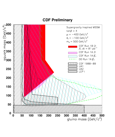
Figure 1.5: Left: The CDF limits on $\sigma\cdot{\rm BR}$ for the $\tilde{\chi}_{2}^{0}\tilde{\chi}_{1}^{+}$ production from the search for trilepton events, eq.(1.47); Right: The CDF limits on the squark and gluino mass including the (jets+$\hbox to0.0pt{\hbox{$\mskip 3.0mu/$}\hss}E_{T}$) and the like-sign lepton signal for the gluino pair production [7]. In part of the parameter space the NLO cross sections have been used [8].

Squarks and Gluinos

The gluino will in general be assumed heavy, as suggested by SUSY-GUT scenarios. The experimental exclusion limits from the direct search for squarks and gluinos are given in the mass plane in Fig. 1.5. The absolute lower limit on the gluino mass is $m_{\tilde{g}}>180{\rm\,GeV}$ [7]. The decay channels considered for the light-flavor squarks and for the gluinos are

$$\tilde{q} \longrightarrow\;q\tilde{\chi}_{j}^{0},\;q^{\prime}\tilde{\chi}_{j}^{+} \longrightarrow \;{\rm jets}+\hbox to0.0pt{\hbox{$\mskip 3.0mu/$}\hss}E_{T}+\cdots$$

$$\tilde{g} \longrightarrow\;q\bar{q}\tilde{\chi}_{j}^{0},\;q^{\prime}\bar{q}\tilde{\chi}_{j}^{+} \longrightarrow \;{\rm jets}+\hbox to0.0pt{\hbox{$\mskip 3.0mu/$}\hss}E_{T}+\cdots$$

$$\tilde{g} \longrightarrow\;q^{\prime}\bar{q}\tilde{\chi}_{j}^{+} \longrightarrow \;{\rm jets}+\hbox to0.0pt{\hbox{$\mskip 3.0mu/$}\hss}E_{T}+\ell\ell\cdots$$

$$\tilde{g} \longrightarrow\;\tilde{t}_{1}\bar{t} \longrightarrow \;b\tilde{\chi}_{j}^{+}\bar{t}\cdots$$ (1.48)

The final state neutralino/chargino decays via a cascade to the lightest neutralino, which is assumed to be the LSP. Products in this decay chain are denoted by the dots. If it is not kinematically forbidden, the gluino can first decay into a squark and a quark, and vice versa. This leads to one more jet in the final state. The stop decay channel of the gluino leads to a higher multiplicity of Standard model particles and bottom jets. A typical signature for the Majorana gluinos arises from the decay via a chargino. Since the gluino is a singlet under the electro-weak gauge group, it decays to $\tilde{\chi}_{j}^{+}$ and $\tilde{\chi}_{j}^{-}$ with the same probability, leading to like-sign leptons in the final state of gluino pair production. A considerable Standard Model background is not present for this signature.

Since supergravity inspired SUSY-GUT relations are used for the experimental search at hadron colliders, there are no strong limits on the squark mass if the gluino mass exceeds $550{\rm\,GeV}$, see Fig. 1.5. The supergravity inspired GUT scenarios as described in section 1.3 do not allow for a gluino mass being much larger than the light-flavor squark mass. In this region of the ($m_{\tilde{q}}-m_{\tilde{g}}$) plane only the general unification of the gaugino masses can be kept. The mass of the lightest neutralino, assumed to be the LSP, grows with the gluino mass and becomes large enough for the squark to decay into an LSP almost at rest. The missing transverse momentum would then become too small to be measured.

The limits on the neutralino/chargino mass from the search at LEP could be translated into limits on the gluino mass, using the gauge coupling unification eq.(1.40). Those are much stricter than the Tevatron limits but model dependent.

Stops

The limits on the stop mass arise from a search for stop pairs decaying into $\tilde{t}_{1}\to c\tilde{\chi}_{1}^{0}$ and are therefore strongly dependent on the mass of the lightest neutralino. For a light stop mass this decay mode will be dominant. In this mass regime the light stop can be produced at LEP $e^{+}e^{-}\to\tilde{t}_{1}\bar{\tilde{t}}_{1}$, Fig. 1.6 [9]. The production cross section depends on the mixing angle, arising from the $\tilde{t}_{1}\tilde{t}_{1}Z$ coupling, and thereby also the mass bound. As will be shown in chapter 4, the hadroproduction cross section is independent of the mixing angle, and both analyses, at LEP and at the Tevatron, yield a mass bound on the lightest stop $m_{\tilde{t}_{\scriptscriptstyle 1}}$ around $79{\rm\,GeV}$ [9, 7]. However, these limits are only valid as long as the $\tilde{\chi}_{1}^{0}$ is light enough and the decay channel $\tilde{t}_{1}\to c\tilde{\chi}_{1}^{0}$ is dominant. Additional limits arising from the search for the decay $t\to\tilde{t}_{1}\tilde{\chi}_{1}^{0}$ are strongly dependent on the branching ratio of this decay mode and therefore weaker than those from the direct search. The different stop decay modes are described in chapter 3, and the direct search at hadron colliders is investigated in chapter 4.

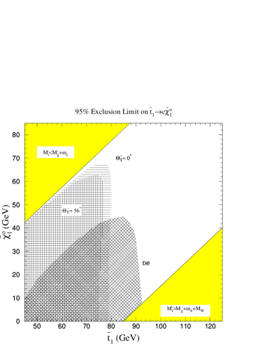
Figure 1.6: Mass limits from the $\tilde{t}_{1}$ pair production at D0 and LEP followed by the decay $\tilde{t}_{1}\to c\tilde{\chi}_{1}^{0}$. The dependence on the mixing angle enters through the coupling $\tilde{t}_{1}\tilde{t}_{1}Z$ at LEP.

1.5 Regularization and Supersymmetric Ward Identities

Dimensional Regularization and Reduction

The $\overline{{\rm MS}}$ renormalization scheme is by definition related to the regularization of infrared and ultraviolet divergences in dimensional regularization (DREG) [35]. This regularization scheme respects gauge symmetry and therefore the gauge symmetry Ward identities. It is less well-suited for supersymmetric theories, since all Lorentz indices are evaluated in $n$ dimensions, whereas the spinors are still four dimensional. This leads to a mismatch between the degrees of freedom carried e.g. by a physical gluon ($n-2$) and a gluino (2). A modified dimensional reduction scheme (DRED) has been introduced to cope with this problem [37]. The number of space-time dimensions is compactified from four to $n$ dimensions, leaving the number of gauge fields invariant i.e. the gauge fields carry the $n$ dimensional Lorentz indices. The remaining ($4-n$) dimensions form the $\epsilon$ scalars. These particles render the $\gamma$ algebra four dimensional. The gauge bosons and the gauginos carry the same number of 4 degrees of freedom. The DRED scheme will be used to illustrate the modified $\overline{{\rm MS}}$ scheme. Except for the unsolved problem of mass factorization in DRED [38, 8] it can be shown that both dimension based schemes are consistent for calculations in the framework of supersymmetric gauge theories.

Starting with a Lagrangean ${\cal L}[W^{a}_{\mu},\lambda^{a},D]$ for a non-abelian supersymmetric gauge theory in the Wess-Zumino gauge one can show that the supersymmetric variation $\delta_{S}$ of the Lagrangean only vanishes in the limit of ($n\to 4$) dimensions, up to a total derivative [39]

$$\delta_{S}{\cal L}[W^{a}_{\mu},\lambda^{a},D]\;\stackrel{{\scriptstyle n\to 4}}{{\longrightarrow}}\;0$$ (1.49)

The component fields $W$ indicate the gauge fields, and $\lambda$ the [Majorana] gauginos. This leads to the Ward identity including the ghost and gauge fixing term ${\cal L}_{G}$, where in $n$ dimensions the variation $\delta_{S}{\cal L}$ has to be kept.

$$0= \;\langle\;\int d^{n}x\left[J^{\mu}\;\delta_{S}W_{\mu}+\bar{j}\;\delta_{S}\lambda+\bar{j}_{D}\;\delta_{S}D+\delta_{S}{\cal L}_{G}+\delta_{S}{\cal L}\right]\;\rangle$$

$$\langle X\rangle\equiv\;\int d\{W_{\mu}\}d\{\lambda\}d\{D\}X\;e^{i\int d^{n}x[{\cal L}+{\cal L}_{G}+J^{\mu}W_{\mu}+\bar{j}\lambda+\bar{j}_{D}D]}$$ (1.50)

Although DREG and thereby the $\overline{{\rm MS}}$ scheme cannot be shown being inconsistent with supersymmetry, they do not respect supersymmetry on the level of naively used Feynman rules. The problem is similar to applying DRED to gauge theories: Evanescent couplings renormalize in a manner different from the physical couplings . In NLO-DREG this results in a finite renormalization of Feynman diagrams which restores supersymmetry explicitly. At higher orders these additional counter terms even include poles in $\epsilon$.

Finite Renormalization

Explicit calculations show that Green’s functions calculated from the MSSM Lagrangean using dimensional regularization may not respect supersymmetry. The supersymmetry transformation mirrors e.g. the gauge coupling $g(qqg)$ to the gauge coupling $g(\tilde{q}\tilde{q}g)$ and the Yukawa coupling $\hat{g}(q\tilde{q}\tilde{g})$. In regularization schemes which respect supersymmetry, like dimensional reduction, the supersymmetric limits of these couplings are identical in any order perturbation theory. In DREG the supersymmetric limit of the Yukawa coupling differs from the gauge couplings at one loop level [40]

$$\hat{g}=g\left[1+\frac{g^{2}}{32\pi^{2}}\left(\frac{4}{3}C(G)-C(r)\right)\right]$$ (1.51)

The Casimir invariants $C$ are defined for the Dirac fermions in the fundamental $(r)$, and for the gauge boson and the Majorana gauge fermions in the adjoint ($G$) representation. This difference has to be compensated to render the calculation supersymmetric. Since the Standard Model quark-gluon coupling $g(qqg)$ is by definition the measured quantity, the Yukawa coupling will be shifted $\hat{g}\to g$ in the expression for the final observable. This finite shift is not a finite field theoretical renormalization of any measured parameter and it is not only present for gauge vs. Yukawa couplings. It is an artifact arising from the supersymmetry violation of naive dimensional regularization.

Supersymmetry relates the weak Higgs Yukawa coupling $Y(qqh)$ to the vertices $Y(\tilde{q}\tilde{q}h)$ and $Y(g\tilde{q}\tilde{h})$. The three couplings $Y$ in the supersymmetric limit and calculated in DREG are not identical in NLO

$$Y(qqh)=Y(\tilde{q}\tilde{q}h)\left[1+\frac{g^{2}}{16\pi^{2}}C(r)\right]=Y(q\tilde{q}\tilde{h})\left[1+\frac{3g^{2}}{32\pi^{2}}C(r)\right]$$ (1.52)

where in the case of weak coupling only $C(r)$ occurs. These two finite differences $\propto\alpha_{s}$ in couplings mediated by $G_{F}$ have to be compensated to make dimensional regularization compatible with supersymmetry.

The usual parameterization of the Yukawa coupling constant is $Y=mg$, where $g$ is defined in the $\overline{{\rm MS}}$ scheme and $m$ is the pole mass, i.e. renormalized in the on-shell scheme. However, the pole mass has to be calculated in the DREG scheme, and the mass appearing in the different couplings eq.(1.52) is — in the supersymmetric limit — only numerically the same. In fact, the scalar mass set to $m$ and the fermion mass set to $m$ behave differently in next-to-leading order, since the counter term for the scalar and the fermion on-shell mass in DREG is not the same.

$$m_{q}=\left[1+\frac{g^{2}}{16\pi^{2}}C(r)\right]\,m_{\tilde{q}}$$ (1.53)

This behavior breaks supersymmetry explicitly and has therefore be removed. The mass shift is responsible for the difference between $Y(qqh)$ and $Y(\tilde{q}\tilde{q}h)$, and it renders the difference to $Y(q\tilde{q}\tilde{h})$ compatible with the general difference between the gauge and Yukawa coupling as given in eq.(1.51):

$$g(qqh)=g(\tilde{q}\tilde{q}h)=g(q\tilde{q}\tilde{h})\left[1+\frac{g^{2}}{32\pi^{2}}C(r)\right]$$ (1.54)

The observable coupling is again defined as in the Standard Model value $Y(qqh)$.

Chapter 2 Production of Neutralinos and Charginos

2.1 Born Cross Sections

Partonic Cross Sections

Neutralinos and Charginos can be produced at hadron colliders in several combinations, all starting from a pure quark incoming state

$$q\,\bar{q}\; \longrightarrow\;\tilde{\chi}_{i}^{0}\tilde{\chi}_{j}^{0}$$

$$q\,\bar{q}\; \longrightarrow\;\tilde{\chi}_{i}^{+}\tilde{\chi}_{j}^{-}$$

$$u\,\bar{d}\; \longrightarrow\;\tilde{\chi}_{i}^{+}\tilde{\chi}_{j}^{0}$$

$$d\,\bar{u}\; \longrightarrow\;\tilde{\chi}_{i}^{-}\tilde{\chi}_{j}^{0}$$ (2.1)

The first two processes are possible for a general quark-antiquark pair. For the latter, charge conservation requires $u$ and $d$ type quarks in the initial state [41].

Figure 2.1: Generic Born diagrams for neutralino/chargino production

Two generic Born Feynman diagrams contribute [Fig. 2.1]: an $s$ channel gauge boson ($\gamma,W,Z$) Drell-Yan like and ($t,u$) channel squark exchange diagrams. Two final state neutralinos are produced by the first diagram purely as higgsino-type. Final state charginos can couple to the $s$ channel gauge boson as gauginos and as higgsinos. For mixed neutralino/chargino production the $s$ channel diagram contributes to all current eigenstates as well. In the given approximation of a trivial squark CKM matrix, the $t,u$ channel squark couples flavor conserving to the incoming quark and will therefore be regarded as light-flavored; the incoming quark originates in the parton density of the proton, and will consistently be assumed massless. This makes the higgsino Yukawa coupling vanish for all possible final states. For the gaugino-like charginos this coupling also vanishes in case of $\tilde{q}_{\scriptscriptstyle R}$, since the $q\tilde{q}\tilde{\chi}$ coupling respects the helicity eigenstates.

The LO partonic cross section $\hat{\sigma}$, which is proportional to the matrix element squared in the limit of $(n\to 4)$ dimensions can for all possible final states be written as [The $n$ dimensional Born cross section is required for the NLO contribution.]

$$\frac{d\hat{\sigma}_{ij}}{dt}=\;\frac{2\pi\alpha^{2}}{Ns^{2}} \Bigg{[}\;\;\frac{2m_{i}m_{j}}{t_{\tilde{q}}}\left(A_{Li}A_{Lj}^{*}C_{T2}+A_{Ri}A_{Rj}^{*}C_{T4}\right)+\frac{2t_{i}t_{j}}{st_{\tilde{q}}}\left(A_{Li}A_{Lj}^{*}C_{T1}+A_{Ri}A_{Rj}^{*}C_{T3}\right)$$

$$-\frac{2m_{i}m_{j}}{u_{\tilde{q}}}\left({A^{c}}_{Lj}{A^{c}}_{Li}^{*}C_{T1}+{A^{c}}_{Rj}{A^{c}}_{Ri}^{*}C_{T3}\right)-\frac{2u_{i}u_{j}}{su_{\tilde{q}}}\left({A^{c}}_{Lj}{A^{c}}_{Li}^{*}C_{T2}+{A^{c}}_{Rj}{A^{c}}_{Ri}^{*}C_{T4}\right)$$

$$+\frac{t_{i}t_{j}+u_{i}u_{j}}{s^{2}}C_{S1}+\frac{m_{i}m_{j}}{s}C_{S2}+\frac{2(u_{1}u_{2}-t_{1}t_{2})}{s(s-M^{2})}C_{S3}$$

$$-\frac{8sm_{i}m_{j}}{t_{\tilde{q}}u_{\tilde{q}}}\left(A_{Lj}A_{Li}^{*}{A^{c}}_{Lj}{A^{c}}_{Li}^{*}+A_{Rj}A_{Ri}^{*}{A^{c}}_{Rj}{A^{c}}_{Ri}^{*}\right)$$

$$+\frac{8t_{i}t_{j}}{t_{\tilde{q}}^{2}}\left(A_{Li}A_{Li}^{*}A_{Lj}A_{Lj}^{*}+A_{Ri}A_{Ri}^{*}A_{Rj}A_{Rj}^{*}\right)$$

$$+\frac{2m_{i}m_{j}}{t_{\tilde{q}}}\left(A_{Lj}A_{Li}^{*}C_{T2}^{*}+A_{Rj}A_{Ri}^{*}C_{T4}^{*}\right)+\frac{2t_{i}t_{j}}{st_{\tilde{q}}}\left(A_{Lj}A_{Li}^{*}C_{T1}^{*}+A_{Rj}A_{Ri}^{*}C_{T3}^{*}\right)$$

$$-\frac{8sm_{i}m_{j}}{t_{\tilde{q}}u_{\tilde{q}}}\left(A_{Li}A_{Lj}^{*}{A^{c}}_{Li}{A^{c}}_{Lj}^{*}+A_{Ri}A_{Rj}^{*}{A^{c}}_{Ri}{A^{c}}_{Rj}^{*}\right)$$

$$+\frac{8t_{i}t_{j}}{u_{\tilde{q}}^{2}}\left({A^{c}}_{Li}{A^{c}}_{Li}^{*}{A^{c}}_{Lj}{A^{c}}_{Lj}^{*}+{A^{c}}_{Ri}{A^{c}}_{Ri}^{*}{A^{c}}_{Rj}{A^{c}}_{Rj}^{*}\right)$$

$$+\frac{2m_{i}m_{j}}{u_{\tilde{q}}}\left({A^{c}}_{Li}{A^{c}}_{Lj}^{*}C_{T1}^{*}+{A^{c}}_{Ri}{A^{c}}_{Rj}^{*}C_{T3}^{*}\right)+\frac{2t_{i}t_{j}}{su_{\tilde{q}}}\left({A^{c}}_{Li}{A^{c}}_{Lj}^{*}C_{T2}^{*}+{A^{c}}_{Ri}{A^{c}}_{Rj}^{*}C_{T4}^{*}\right)\Bigg{]}$$

$$\qquad\text{where}\qquad t_{\tilde{q}}=t-m_{\tilde{q}}^{2}\qquad u_{\tilde{q}}=u-m_{\tilde{q}}^{2}$$ (2.2)

$M$ is the $W$ or $Z$ mass of the $s$ channel gauge boson. The coupling parameters $A$ correspond to the $t,u$ channel couplings for the outgoing particles $i,j$ and are defined in Tab. A.5. The charge conjugate coupling $A^{c}$ is identical to $A$ for the neutralinos. In the chargino case $A_{j}$ is the coupling for outgoing $\tilde{\chi}_{j}^{-}$ containing the mixing matrix $U$, and ${A^{c}}_{j}$ for an outgoing $\tilde{\chi}_{j}^{+}$ containing $V$. The typical couplings $C_{S},C_{T}$ follow from the Feynman rules Fig. 2.1:

$$C_{S1}= \;X_{c}^{2}-\frac{X_{c}s}{2(s-M^{2})}\,\text{Re\,}\left[(\ell+r)(L+R)\right]+\frac{s^{2}}{4(s-M^{2})^{2}}\,(|\ell|^{2}+|r|^{2})\,(|L|^{2}+|R|^{2})$$

$$C_{S2}= \;X_{c}^{2}-\frac{X_{c}s}{2(s-M^{2})}\,\text{Re\,}\left[(\ell+r)(L+R)\right]+\frac{s^{2}}{2(s-M^{2})^{2}}\,(|\ell|^{2}+|r|^{2})\,\,\text{Re\,}\left[|L||R|\right]$$

$$C_{S3}= \;\frac{X_{c}}{4}\,\text{Re\,}\left[(\ell-r)(L-R)\right]+\frac{s}{8(s-M^{2})}\,(|\ell|^{2}-|r|^{2})\,(|L|^{2}-|R|^{2})$$

$$C_{T1}= \;X_{c}+\frac{s}{s-M^{2}}\;\ell R\qquad\qquad\qquad C_{T2}=\;X_{c}+\frac{s}{s-M^{2}}\;\ell L$$

$$C_{T3}= \;X_{c}+\frac{s}{s-M^{2}}\;rL\qquad\qquad\qquad C_{T4}=\;X_{c}+\frac{s}{s-M^{2}}\;rR$$

$$X_{c}= \;-Q\qquad\text{only for}\quad\tilde{\chi}_{j}^{-}\tilde{\chi}_{j}^{+}$$ (2.3)

The gauge boson-quark couplings $r,\ell$ are given in Tab. A.2, the neutralino-chargino couplings in Tab. A.4. Final state charginos require one subtlety in the matrix elements: either the $t$ or the $u$ channel diagrams contribute to the amplitude with a fixed quark flavor, except for the pure neutralino case. For two final state charginos, $A$ only couples to $u$ type, ${A^{c}}$ to $d$ type quarks. In the mixed production processes the couplings $A$ and ${A^{c}}$ have to be arranged making use of charge conservation.

The factor of $C_{S3}$ in the Born cross section eq.(2.2) originates from the contraction of two CP odd Dirac traces ${\rm Tr}(\gamma_{5}\gamma^{\mu}\hbox to0.0pt{\hbox{$\mskip 1.0mu/$}\hss}k_{1}\gamma^{\nu}\hbox to0.0pt{\hbox{$\mskip 1.0mu/$}\hss}k_{2}){\rm Tr}(\gamma_{5}\gamma^{\mu}\hbox to0.0pt{\hbox{$\mskip 1.0mu/$}\hss}p_{1}\gamma^{\nu}\hbox to0.0pt{\hbox{$\mskip 1.0mu/$}\hss}p_{2})$, where the definition of the momenta is given in appendix B.1. Using a naive $\gamma_{5}$ scheme, this term cannot be fixed consistently. We therefore keep this kind of structure in the Born, real gluon and virtual gluon contributions. The different choices for the $\gamma_{5}$ scheme result in ${\cal O}(\epsilon)$ corrections and do not contribute to the final expression, since the corresponding diagrams are finite. The calculation performed in the consistent ’t Hooft-Veltman scheme [35] agrees with the naive calculation.

Hadronic Cross Section

The hadronic cross section for $pp/p\bar{p}$ collisions is given by a convolution of the partonic cross section with the parton densities for the quarks in the proton, e.g. for two hadrons $H_{1}H_{2}$

$$\sigma(S,Q^{2})=\sum_{{\rm partons\,}ij}\;\int_{\tau_{0}}^{1}dx_{i}\int_{\frac{\tau_{0}}{x_{i}}}^{1}dx_{j}\;\left[f^{H_{1}}_{i}(x_{i},Q^{2})\,f^{H_{2}}_{j}(x_{j},Q^{2})+(H_{1}\leftrightarrow H_{2})\right]\;\hat{\sigma}_{ij}(x_{i}x_{j}S,Q^{2})$$ (2.4)

where $k_{1}$ and $k_{2}$ are the incoming parton momenta, $S=(k_{1}+k_{2})^{2}$ is the hadronic cm energy; $m_{j}$ are the masses of the final state particles, and $\tau_{0}=(m_{1}+m_{2})^{2}/S$ is the kinematical limit. $f^{H_{j}}_{i}$ are the parton densities, forming the convoluted hadronic luminosity

$$\sigma(S,Q^{2})\,=\sum_{{\rm partons\,}ij}\;\int_{\tau_{0}}^{1}d\tau\;\frac{d{\cal L}_{ij}}{d\tau}(\tau,Q^{2})\;\hat{\sigma}_{ij}(\tau S,Q^{2})$$

$$\frac{d{\cal L}_{ij}}{d\tau}(\tau,Q^{2})\,=\left[f_{i}\otimes f_{j}\right](\tau,Q^{2})+\left[f_{j}\otimes f_{i}\right](\tau,Q^{2})$$

$$\left[f\otimes g\right](\tau,Q^{2})\equiv\int_{\tau}^{1}\frac{dx}{x}\,f(x,Q^{2})\,g\left(\frac{\tau}{x},Q^{2}\right)$$ (2.5)

where the hadrons $H_{1},H_{2}$ are implicitly fixed by the order of the convolution of the parton densities. For identical incoming gluons a factor 1/2 has to be incorporated.

2.2 Next-to-leading Order Cross Sections

2.2.1 Virtual and Real Gluon Emission

The NLO cross section includes the radiation of real quarks and gluons and virtual gluons and gluinos. The generic diagrams are given in Fig. 2.2 for the $q\bar{q}$ incoming state. The additional $qg$ and $g\bar{q}$ diagrams are obtained by crossing one quark to the final and the gluon to the initial state. The virtual contributions are regularized by dimensional regularization. Therefore a finite shift of the couplings eq.(1.52) has to be applied to restore supersymmetry. The divergences appear as poles in $\epsilon$, as shown in appendix B.3. The UV poles require renormalization; the only parameter in the Born term eq.(2.2) which undergo the renormalization procedure is the squark mass, defined as the pole mass, i.e. in the on-shell scheme. The soft gluon poles cancel with the real gluon emission. The phase space integration for the real gluon emission is given in appendix B.1. These matrix elements have been computed using phase space subtraction, i.e. the additional gluon phase space is integrated numerically. After subtracting the dipole terms the remaining divergences are of collinear type and removed by mass factorization, appearing in the subtraction term, see appendix B.1.

Figure 2.2: Generic NLO diagrams for neutralino/chargino production, the self energy contributions are not shown.

2.2.2 Mass Factorization

The parton densities eq.(2.5) form observable structure functions [e.g. $F_{2}$], which contain divergences in next-to-leading order QCD [54]. These divergences arise from the collinear radiation of gluons and have a universal structure which is fixed by the $Q^{2}$ evolution. They have to be absorbed into the definition of the parton densities to render the physical structure function finite. In analogy to a UV renormalization procedure it is possible to absorb additional finite parts into the re-definition. The minimal set is the $\overline{{\rm MS}}$ scheme, and it leaves the next-to-leading order contribution to the measured structure function with a non-zero finite term. This minimal choice respects the required sum rules naively.

Due to the factorization theorem, the universal form of the partonic cross section in the collinear limit is independent of the order of perturbation theory.

$$s^{2}\frac{d^{2}\hat{\sigma}_{ij}}{dt_{2}ds_{4}}= \;\int_{0}^{1}\frac{dx_{i}}{x_{i}}\int_{0}^{1}\frac{dx_{j}}{x_{j}}\;\Gamma_{li}(x_{i},Q^{2})\,\Gamma_{mj}(x_{j},Q^{2})\left(s^{2}\frac{d^{2}\hat{\sigma}_{lm}^{\rm red}}{dt_{2}ds_{4}}\right)_{x_{i}k_{i},x_{j}k_{j}}$$

$$\Gamma_{ij}(x,Q^{2})=\;\delta_{ij}\,\delta(1-x)-\frac{\alpha_{s}}{2\pi\epsilon}\,\frac{\Gamma(1-\epsilon)}{\Gamma(1-2\epsilon)}\left(\frac{4\pi Q^{2}}{Q_{F}^{2}}\right)^{\epsilon}P_{ij}(x)$$ (2.6)

$\Gamma_{ij}$ is called splitting function and describes the splitting of a parton $i$ to a parton $j$ in the collinear limit. It is evaluated perturbatively and consists of the trivial LO term and a divergent NLO contribution. The appearance of the Altarelli-Parisi kernels $P_{ij}$ fixes the $Q^{2}$ evolution, they are given in eq.(B.23). Other non-minimal schemes lead to a finite renormalization $\Gamma_{ij}\to\Gamma_{ij}+f_{ij}$. The reduced cross section $\hat{\sigma}^{\rm red}$ is finite and, as well as the splitting function, depends on the factorization scale $Q_{F}$. This scale dependence should flatten after adding higher order perturbative contributions, since it is a perturbative artifact.

The renormalization of the parton densities has to cancel the remaining collinear poles in the matrix elements and leave the final expression finite. The counter term which has to be added to the bare cross section to obtain the reduced one in the $\overline{{\rm MS}}$ scheme can be read off eq.(2.6)

$$s^{2}\frac{d^{2}\hat{\sigma}^{MF}_{ij}}{dt_{2}ds_{4}}=\frac{\alpha_{s}}{2\pi\epsilon}\frac{\Gamma(1\!-\!\epsilon)}{\Gamma(1\!-\!2\epsilon)}\left(\frac{4\pi Q^{2}}{Q_{F}^{2}}\right)^{\epsilon}\int_{0}^{1}\frac{dx}{x}\left[P_{li}(x)\!\left(s^{2}\frac{d^{2}\hat{\sigma}^{B}_{lj}}{dt_{2}ds_{4}}\right)_{xk_{l}}+P_{mj}(x)\!\left(s^{2}\frac{d^{2}\hat{\sigma}^{B}_{im}}{dt_{2}ds_{4}}\right)_{xk_{m}}\right]$$

2.2.3 On-Shell Subtraction

Figure 2.3: Feynman diagrams for crossed channel production of neutralinos/charginos including on-shell intermediate states, which have to be subtracted.

Apart from the UV and IR divergences another kind of divergences can occur, due to on-shell intermediate particles. After crossing the NLO production matrix elements, different incoming states may contribute to the ($\chi\chi$+jet) inclusive final state

$$qg \longrightarrow\chi_{i}\chi_{j}q$$

$$g\bar{q} \longrightarrow\chi_{i}\chi_{j}\bar{q}$$ (2.8)

As depicted in Fig. 2.3, these can proceed via an on-shell squark. A natural way of solving the problem would be introducing finite widths for all particles under consideration. However, a finite squark width would spoil gauge invariance. In addition, it would yield a strong dependence of the next-to-leading order production cross section on the physical widths of intermediate states. This dependence would only vanish after including the decays into the calculation. Therefore we instead differentiate between off-shell and on-shell particle contributions, the latter regarded as final states in the set of supersymmetric production cross sections.

Considering an analysis of all production processes for two MSSM particles at hadron colliders this differentiation removes a double counting of the on-shell contributions of the squark, as it would occur in the case of general finite widths:

$$gq\to\tilde{q}^{*}\chi_{i}\to q\chi_{j}\chi_{i}\quad$$ neutralino pair production

$$gq\to\tilde{q}\chi_{i}\cdot{\rm BR}(\tilde{q}\to q\chi_{j})\quad$$ squark neutralino production (2.9)

The on-shell squark contribution is subtracted from the crossed $\chi_{i}\chi_{j}$ production matrix element, leaving it as a contribution to direct $\chi\tilde{q}$ production, eq.(2.9). The off-shell contribution is kept for the first of the processes under consideration. To distinguish these contributions numerically, one regularizes the possibly divergent propagator by introducing the Breit-Wigner propagator $(p^{2}-m^{2})\to(p^{2}-m^{2}+im\Gamma)$. Since this width can be regarded not as a physical property of the final state particle, but as a mathematical cut-off, the matrix element can be evaluated in the narrow width approximation, regarding the final state particles as quasi-stable.

Assuming an on-shell divergence in the variable $M^{2}$, the hard production cross section in the narrow width approximation reads

$$\frac{d\sigma}{dM^{2}} =\;\sigma\left(gq\to\tilde{q}\chi_{i}\right)\,\frac{m_{\tilde{q}}\Gamma_{\tilde{q}}/\pi}{(M^{2}-m_{\tilde{q}}^{2})^{2}+m_{\tilde{q}}^{2}\Gamma_{\tilde{q}}^{2}}\,{\rm BR}\left(\tilde{q}\to q\chi_{j}\right)+{\cal O}\left(\frac{1}{M^{2}-m_{\tilde{q}}^{2}}\right)$$

$$\longrightarrow\;\sigma\left(gq\to\tilde{q}\chi_{i}\right)\,{\rm BR}\left(\tilde{q}\to q\chi_{j}\right)\,\delta(M^{2}-m_{\tilde{q}}^{2})+{\cal O}\left(\frac{1}{M^{2}-m_{\tilde{q}}^{2}}\right)$$ (2.10)

Figure 2.4: The renormalization/factorization scale dependence of the total cross section for $\tilde{\chi}_{2}^{0}\tilde{\chi}_{1}^{+}$ production at the upgraded Tevatron and the LHC. There is no maximum in either of the next-to-leading order curves, and the LO and NLO do not meet for a scale around the average mass. The SUSY scenario determining the masses is given in eq.(1.45).

In case of the neutralino/chargino production $M^{2}=s_{3}+m_{1}^{2}$ and $M^{2}=s_{4}+m_{2}^{2}$ are relevant for the on-shell squarks, the extended set of Mandelstam variables is defined in appendix B. The leading divergence is subtracted from the crossed channel matrix element, as described before. The complete crossed channel matrix element can be written as $|{\cal M}|^{2}=f(M^{2})/[(M^{2}-m_{\tilde{q}}^{2})^{2}+m_{\tilde{q}}^{2}\Gamma_{\tilde{q}}^{2}]$; then the subtraction for an intermediate squark is defined as

$$\frac{f(M^{2})}{(M^{2}-m_{\tilde{q}}^{2})^{2}+m_{\tilde{q}}^{2}\Gamma_{\tilde{q}}^{2}}\,-\,\frac{f(m_{\tilde{q}}^{2})}{(M^{2}-m_{\tilde{q}}^{2})^{2}+m_{\tilde{q}}^{2}\Gamma_{\tilde{q}}^{2}}\,\Theta(\hat{s}-(m_{\tilde{q}}+m_{i})^{2})\,\Theta(m_{\tilde{q}}-m_{j})$$ (2.11)

Since an over-all factor $\delta(M^{2}-m_{\tilde{q}}^{2})$ is absent in the subtracted term, the Breit-Wigner propagator has to be integrated over the phase space variable $M^{2}$. The matrix element, including the remaining phase space integration is evaluated for $M^{2}=m_{\tilde{q}}^{2}$.

The remaining non-leading divergences, arising from interference between finite and divergent Feynman diagrams, are integrable and well-defined using a principal-value integration. Numerically this principal value can be implemented by introducing a small imaginary part ($M^{2}\to M^{2}-i\varepsilon$). Since the matrix element squared may contain subtractions in more than one variable this imaginary part may lead to finite contributions and has therefore to be taken into account.

2.3 Results

$\tilde{\chi}_{i}^{0}\tilde{\chi}_{j}^{0}$	$K_{\rm LHC}$	$\tilde{\chi}_{i}^{0}\tilde{\chi}_{j}^{+}$	$K_{\rm LHC}$	$\tilde{\chi}_{i}^{0}\tilde{\chi}_{j}^{-}$	$K_{\rm LHC}$	$\tilde{\chi}_{i}^{+}\tilde{\chi}_{j}^{-}$	$K_{\rm LHC}$
$\tilde{\chi}_{1}^{0}\tilde{\chi}_{1}^{0}$	1.51	$\tilde{\chi}_{1}^{0}\tilde{\chi}_{1}^{+}$	1.35	$\tilde{\chi}_{1}^{0}\tilde{\chi}_{1}^{-}$	1.37	$\tilde{\chi}_{1}^{+}\tilde{\chi}_{1}^{-}$	1.33
$\tilde{\chi}_{1}^{0}\tilde{\chi}_{2}^{0}$	1.50	$\tilde{\chi}_{2}^{0}\tilde{\chi}_{1}^{+}$	1.33	$\tilde{\chi}_{2}^{0}\tilde{\chi}_{1}^{-}$	1.34	$\tilde{\chi}_{1}^{+}\tilde{\chi}_{2}^{-}$	1.44
$\tilde{\chi}_{1}^{0}\tilde{\chi}_{3}^{0}$	1.35	$\tilde{\chi}_{3}^{0}\tilde{\chi}_{1}^{+}$	1.35	$\tilde{\chi}_{3}^{0}\tilde{\chi}_{1}^{-}$	1.33	$\tilde{\chi}_{2}^{+}\tilde{\chi}_{1}^{-}$	1.41
$\tilde{\chi}_{1}^{0}\tilde{\chi}_{4}^{0}$	1.39	$\tilde{\chi}_{4}^{0}\tilde{\chi}_{1}^{+}$	1.90	$\tilde{\chi}_{4}^{0}\tilde{\chi}_{1}^{-}$	1.98	$\tilde{\chi}_{2}^{+}\tilde{\chi}_{2}^{-}$	1.32
$\tilde{\chi}_{2}^{0}\tilde{\chi}_{2}^{0}$	1.44	$\tilde{\chi}_{1}^{0}\tilde{\chi}_{2}^{+}$	1.38	$\tilde{\chi}_{1}^{0}\tilde{\chi}_{2}^{-}$	1.40
$\tilde{\chi}_{2}^{0}\tilde{\chi}_{3}^{0}$	1.35	$\tilde{\chi}_{2}^{0}\tilde{\chi}_{2}^{+}$	2.51	$\tilde{\chi}_{2}^{0}\tilde{\chi}_{2}^{-}$	2.65
$\tilde{\chi}_{2}^{0}\tilde{\chi}_{4}^{0}$	1.45	$\tilde{\chi}_{3}^{0}\tilde{\chi}_{2}^{+}$	1.35	$\tilde{\chi}_{3}^{0}\tilde{\chi}_{2}^{-}$	1.34
$\tilde{\chi}_{3}^{0}\tilde{\chi}_{3}^{0}$	1.30	$\tilde{\chi}_{4}^{0}\tilde{\chi}_{2}^{+}$	1.31	$\tilde{\chi}_{4}^{0}\tilde{\chi}_{2}^{-}$	1.32
$\tilde{\chi}_{3}^{0}\tilde{\chi}_{4}^{0}$	1.33
$\tilde{\chi}_{4}^{0}\tilde{\chi}_{4}^{0}$	1.38

Table 2.1: A complete set of $K$ factors for neutralino and chargino production at the LHC. The masses are chosen according to the default SUGRA inspired scenario, eq.(1.45). The renormalization and factorization scales are set to the average final state mass. Although the $K$ factors are of a similar size $1.3\cdots 1.5$ for each diagram contributing, large cancelations lead to huge corrections for the scenario under consideration.

Scale Dependence

Since the leading order hadro-production cross section for neutralinos and charginos does not contain the QCD coupling constant, it only depends on the factorization scale through the parton densities. This renders the leading order scale dependence smaller than $\sim 30\%$. The variation of the cross section with the scale is therefore not a good measure for the theoretical uncertainty. In next-to-leading order, this factorization scale dependence becomes weaker; however, an additional dependence on the renormalization scale arises. For $\mu=\mu_{F}=\mu_{R}$ this yields a generally weak scale dependence of $\lesssim 20\%$ at the upgraded Tevatron and $\lesssim 5\%$ at the LHC. As can be seen from the leading order curves in Fig. 2.4, the combination of factorization and renormalization scale dependence leads to a different behavior at the Tevatron and at the LHC, due to different momentum fractions $x$ contributing; in contrast to the strong coupling induced processes a maximum cross section for some small scale does not occur, Fig. 2.4.

Numerical Results

The production of neutralinos and charginos can be probed at the upgraded Tevatron, a $p\bar{p}$ collider with a center-of-mass energy of 2${\rm\,TeV}$, and at the future LHC, a $pp$ collider with an energy of 14${\rm\,TeV}$. The cross section for several combinations of light neutralinos and charginos, which turn out to be gaugino-like in the considered scenario, are given in Fig. 2.5. The size of the cross sections strongly depends on the mixing matrix elements associated with the different couplings. This yields e.g. a larger cross section for $\tilde{\chi}_{2}^{0}\tilde{\chi}_{1}^{+}$ pairs compared to $\tilde{\chi}_{1}^{0}\tilde{\chi}_{1}^{+}$ production. In general, the processes containing no final state chargino are suppressed, independent of the masses, which are almost the same for $\tilde{\chi}_{2}^{0}$ and $\tilde{\chi}_{1}^{+}$. Whereas the cross section for the production of positively and negatively charged mixed pairs are identical at the Tevatron, they differ significantly at the LHC, due to non-symmetric parton luminosities. The dependence on SUSY masses and parameters, which are not contained in the leading order cross section, like the gluino mass, is weak in next-to-leading order. The virtual corrections are generically small [$\lesssim 10\%$] compared to the real gluon emission; however, they are not universal and even do not have a unique sign for the different gaugino and higgsino-type outgoing particles.

The next-to-leading order $K$ factor is consistently defined as $K=\sigma_{NLO}/\sigma_{LO}$. It is dominated by the gluon emission off the incoming partons and therefore similar for all considered processes and a constant function of the masses, Tab. 2.1. Although the real gluon corrections to any diagram contributing to the production process are of the order $1.3\cdots 1.5$, large cancelations give rise to huge $K$ factors. The same effect occurs for the virtual corrections, which grow up to 50$\%$ e.g. for the $\tilde{\chi}_{2}^{0}\tilde{\chi}_{2}^{\pm}$ or the $\tilde{\chi}_{4}^{0}\tilde{\chi}_{1}^{\pm}$ channel. Varying the common gaugino mass $m_{1/2}$ reduces the $K$ factor to values expected by regarding the other channels.

With an integrated luminosity of $\int{\cal L}=20{\rm fb}^{-1}$ in run II, the upgraded Tevatron will have a maximal reach for the mass of the produced particles when probing the $\tilde{\chi}_{2}^{0}\tilde{\chi}_{1}^{+}$ channel. For masses smaller than 150${\rm\,GeV}$, $10^{3}$ to $10^{5}$ events could there be accumulated. Although the $\tilde{\chi}_{1}^{+}\tilde{\chi}_{1}^{-}$ cross section is compatible with the mixed neutralino/chargino channel for a fixed value of the common gaugino mass, the particle masses, which can be probed, stay below 80${\rm\,GeV}$ in the considered SUGRA inspired scenario. The same holds for the LHC, where for typical masses of the $\tilde{\chi}_{1}^{+}$ and $\tilde{\chi}_{2}^{0}$ below 300${\rm\,GeV}$ and an integrated luminosity of $\int{\cal L}=300{\rm fb}^{-1}$ a sample of $10^{4}$ to $10^{6}$ events can be accumulated. In the given scenario the higgsino type neutralinos and charginos are strongly suppressed compared with the lighter gauginos.

Figure 2.5: Some total cross sections for pairs of neutralinos and charginos at the Tevatron and at the LHC as a function of $m_{1/2}$. The different masses of the particles involved are given on secondary axis. The strongly suppressed heavy higgsino cross sections are not given. The $\tilde{\chi}_{2}^{0}\tilde{\chi}_{1}^{+}$ and $\tilde{\chi}_{2}^{0}\tilde{\chi}_{1}^{-}$ cross sections are different due to the non-symmetric parton luminosities.

Chapter 3 Scalar Top Quark Decays

Scalar top quarks can decay into two or three on-shell particles via the strong or electroweak coupling [42]. The possible two body decays are — kinematically allowed for an increasing stop mass in typical mass scenarios:

$$\tilde{t}_{j} \longrightarrow\;c\tilde{\chi}_{1}^{0},\quad b\tilde{\chi}_{i}^{+},\quad t\tilde{\chi}_{i}^{0},\quad[\;Z\tilde{t}_{1},\quad h\tilde{t}_{1},\quad W^{+}\tilde{b},\quad H^{+}\tilde{b},\quad t\tilde{g}\;]$$

$$\tilde{t}_{j} \longrightarrow\;W^{+}b\tilde{\chi}_{1}^{0},\quad H^{+}b\tilde{\chi}_{1}^{0}\quad\cdots$$ (3.1)

The channels in brackets are possible only for the heavier stop, since the $\tilde{t}_{1}$ is assumed to be the lightest scalar quark. The decay into a charm jet is induced by a one-loop amplitude, and will therefore be suppressed, if any other tree-level two or three body decay channel is open. In the intermediate mass range, when the $b\tilde{\chi}_{i}^{+}$ channel is still closed, the three particle decay into $Wb\tilde{\chi}_{1}^{0}$ is dominant. For a heavy $\tilde{t}_{2}$ the strong decay mode including a final state gluino will be the leading one, as will be shown later in this chapter.

3.1 Strong Decays

3.1.1 Born Decay Widths

Since the Yukawa $q\tilde{q}\tilde{g}$ couplings are flavor diagonal, any decay involving a scalar top quark

$$\tilde{t}_{j}\longrightarrow \;t+\tilde{g}\qquad\qquad \left[m_{\tilde{t}_{\scriptscriptstyle j}}>m_{t}+m_{\tilde{g}}\right]$$

$$\tilde{g}\longrightarrow \;\bar{t}+\tilde{t}_{j}\quad\text{and c.c.}\qquad\qquad \left[m_{\tilde{g}}>m_{t}+m_{\tilde{t}_{\scriptscriptstyle j}}\right]$$ (3.2)

includes a top quark in the final state, i.e. the strong decays will only be possible for large mass scenarios. For the light stop $\tilde{t}_{1}$ the weak decays in eq.(3.1) will be the only kinematically allowed.

The calculation including the stop mixing and a massive top quark is a generalization of the light-flavor decay width [43]. To lowest order the partial widths for the stop and gluino decay, eq.(3.2), are given by by

$$\Gamma(\tilde{t}_{1,2}\rightarrow t\,\tilde{g}) =\frac{2\alpha_{s}}{Nm_{\tilde{t}_{\scriptscriptstyle 1,2}}^{3}}\Lambda^{1/2}(m_{\tilde{t}_{\scriptscriptstyle 1,2}}^{2},m_{t}^{2},m_{\tilde{g}}^{2})\left[m_{\tilde{t}_{\scriptscriptstyle 1,2}}^{2}-m_{t}^{2}-m_{\tilde{g}}^{2}\pm 2m_{t}m_{\tilde{g}}\sin(2\tilde{\theta})\right]$$

$$\Gamma(\tilde{g}\rightarrow\bar{t}\,\tilde{t}_{1,2}) =-\frac{\alpha_{s}}{(N^{2}-1)m_{\tilde{g}}^{3}}\Lambda^{1/2}(m_{\tilde{t}_{\scriptscriptstyle 1,2}}^{2},m_{t}^{2},m_{\tilde{g}}^{2})\left[m_{\tilde{t}_{\scriptscriptstyle 1,2}}^{2}-m_{t}^{2}-m_{\tilde{g}}^{2}\pm 2m_{t}m_{\tilde{g}}\sin(2\tilde{\theta})\right]$$ (3.3)

The different factors in front are due to the color and spin averaging of the decaying particle, and the crossing of a fermion line. Interchanging $\tilde{t}_{1}$ and $\tilde{t}_{2}$ in the two leading-order decay widths corresponds to the symmetry operation ${\cal P}_{12}$ in the Lagrangean, as described in section 1.2.4.

3.1.2 Next-to-leading Order SUSY-QCD Corrections

Massive Gluon Emission

The NLO corrections [11] include the emission of an on-shell gluon, Fig. 3.1c. This gluon leads to IR singularities which are regularized using a small gluon mass $\lambda$, subsequently appearing in logarithms $\log\lambda^{2}$. The massive gluon scheme breaks gauge invariance for the non-abelian SU(3) symmetry. Hence the scheme has to be extended by new counter terms if a non-abelian contribution arises from a three or four gluon vertex, otherwise the SU(3) Ward identities would not be satisfied anymore. This is not the case for the stop decays Fig. 3.1. The gluon behaves like a photon and its mass can be regarded as a mathematical cut-off parameter. After integration over the whole phase space the small mass parameter drops out and yields a finite sum of virtual and real gluon matrix elements. However, these massive gluon matrix elements must not be interpreted as exclusive cross sections, since gauge invariance is only restored for inclusive observables, i.e. the gluon integrated out.

In the considered process the logarithms of the gluon mass arise from the integration over the soft and collinear divergent three particle phase space, eq.(B.7). The same kind of logarithms enter through the virtual gluon contributions, e.g. the scalar three point function eq.(B.44) and cancel analytically.

Figure 3.1: (a) Born diagrams for stop and gluino decays; (b) vertex corrections; (c) real gluon emission. The correction to the gluino decay can be obtained by crossing the diagrams

Virtual Corrections

The virtual gluon corrections, including self energy diagrams for all external particles and vertex corrections Fig. 3.1c, are also regularized using the massive gluon scheme. The additional UV divergences have to be regularized dimensionally. The poles $1/\epsilon$ are absorbed into the renormalization of the masses, the strong coupling, and the mixing angle, which are the parameters appearing in the Born decay width eq.(3.3). The counter terms for mass renormalization in the on-shell scheme and the renormalization of $\alpha_{s}$ in $\overline{{\rm MS}}$ can be found in appendix B.4. The mixing angle is renormalized by introducing the running mixing angle and absorbing the mixing stop self energy contributions. This scheme restores the ($\tilde{t}_{1}\leftrightarrow\tilde{t}_{2}$) symmetry ${\cal P}_{12}$ in NLO. The dependence on the mixing angle in NLO can be described by a constant $K$ factor, Fig. 3.2, possibly large contributions from the gluino-top loop are absorbed into the definition of the mixing angle. Renormalizing the strong coupling in the $\overline{{\rm MS}}$ scheme breaks supersymmetry; adding a finite counter term, derived in eq.(1.51), restores supersymmetry.

The Born decay widths are proportional to $\Lambda^{1/2}$, i.e. the relative momentum of the produced particles. One of the vertex correction diagrams is constructed by exchanging a virtual gluon between outgoing color charged particles. Near threshold the exchange of a gluon between two slowly moving particles picks up a factor $\Lambda^{-1/2}$, the Coulomb singularity, which cancels against the phase space suppression factor in the virtual correction matrix element. The NLO decay width therefore does not vanish at threshold. The narrow divergence can be removed by resummation of the contributions near threshold. Moreover, the screening due to a non-zero life time of the final state particles reduces the Coulomb effect considerably.

The complete analytical expression for the stop decay width is given in appendix C. The numerical results are shown together with the weak decays in Fig. 3.3.

Figure 3.2: Left: Renormalization scale dependence of the gluino decay width for the same SUGRA inspired scenario as chosen in Fig. 3.3: $m_{\tilde{t}_{\scriptscriptstyle 1}}=449{\rm\,GeV}$,$m_{\tilde{t}_{\scriptscriptstyle 2}}=847{\rm\,GeV}$, $\sin(2\tilde{\theta})=-0.59$, and $m_{\tilde{g}}=637{\rm\,GeV}$. The renormalization scale is varied as a fraction of the mass of the decaying gluino; Right: mixing angle dependence of this gluino decay, where the stop mixing has been varied over the whole range, independent of the other low energy parameters.

3.2 Weak Decays

The possible weak decay modes including a stop will be dominant once the strong channels are kinematically forbidden. Although this region is not preferred by the mSUGRA scenario even the crossed top decay could be possible, which leads to experimental limits on the branching ratio of this decay mode and thereby on the masses involved [7]

$$\tilde{t}_{j}\longrightarrow \;t+\tilde{\chi}_{j}^{0}\qquad\qquad \left[m_{\tilde{t}_{\scriptscriptstyle j}}>m_{t}+m_{\tilde{\chi}_{\scriptscriptstyle j}}\right]$$

$$\tilde{t}_{j}\longrightarrow \;b+\tilde{\chi}_{j}^{+}\qquad\qquad \left[m_{\tilde{t}_{\scriptscriptstyle j}}>m_{b}+m_{\tilde{\chi}_{\scriptscriptstyle j}}\right]$$

$$t\longrightarrow \;\tilde{t}_{1}+\tilde{\chi}_{j}^{0}\qquad\qquad \left[m_{t}>m_{\tilde{t}_{\scriptscriptstyle 1}}+m_{\tilde{\chi}_{\scriptscriptstyle j}}\right]$$ (3.4)

The Born decay width for the $\tilde{t}_{1}$ decay to a neutralino reads

$$\Gamma(\tilde{t}_{1}\rightarrow t\,\tilde{\chi}_{j}^{0})= \;\frac{2\alpha}{Nm_{\tilde{t}_{\scriptscriptstyle 1}}^{3}}\Lambda^{1/2}(m_{\tilde{t}_{\scriptscriptstyle 1}}^{2},m_{t}^{2},m_{\tilde{\chi}_{\scriptscriptstyle j}}^{2})\left[\left(m_{\tilde{t}_{\scriptscriptstyle 1}}^{2}-m_{t}^{2}-m_{\tilde{\chi}_{\scriptscriptstyle j}}^{2}\right)(C_{L}^{2}+C_{R}^{2})+4m_{t}m_{\tilde{\chi}_{\scriptscriptstyle j}}C_{L}C_{R}\right]$$

$$C_{L}= \;A_{L}\cos\tilde{\theta}+B_{L}\sin\tilde{\theta}$$

$$C_{L}= \;B_{R}\cos\tilde{\theta}-A_{R}\sin\tilde{\theta}$$ (3.5)

The couplings $A$ and $B$ are given in Tab. A.5 for the neutralino involved. The $\tilde{t}_{2}$ decay can be derived using the ${\cal P}_{12}$ operation. The decay channel producing a bottom quark and a chargino can be read off using Tab. A.5 by setting the mixing angle to zero, as long as sbottom mixing is neglected. The NLO calculation is performed exactly as for the strong decay channel, whereby some virtual and real correction diagrams in Fig. 3.1 vanish for a Majorana particle without color charge. Again the finite shift eq.(1.52) has to be added to the weak coupling vertex, no matter if a gaugino or a higgsino is involved.

Figure 3.3: Left: SUSY-QCD corrections to the strong decays $\tilde{t}_{2}\to\tilde{g}t$ and $\tilde{g}\to t\bar{\tilde{t}}_{1}+\bar{t}\tilde{t}_{1}$ as a function of the common gaugino mass. The masses of the particles involved are labeled in the additional axis. The input parameters have been chosen as $m_{0}=900{\rm\,GeV},A_{0}=900{\rm\,GeV},\tan\beta=2.5,\mu>0$, in order to see the possible structures of the curves. The kink in the NLO stop decay width results from the gluino self energy and could be smoothed by inserting a finite gluino width; Right: SUSY-QCD corrections to weak decays of the light $\tilde{t}_{1}$. The input parameters are the usual $m_{0}=100{\rm\,GeV},A_{0}=300{\rm\,GeV},\tan\beta=4,\mu>0$. Only the decay into the two lightest neutralinos and into the light chargino is possible in the $m_{1/2}$ range considered. Note that the mass of the $\tilde{\chi}_{1}^{+}$ and the $\tilde{\chi}_{2}^{0}$ are almost identical in the SUGRA inspired scenario. The dashed line denotes the LO, the solid one the NLO results in both figures.

3.3 Results

In the calculation the renormalization scale of the process is fixed to the mass of the decaying particle. Since the scale dependence should vanish after adding all orders of perturbation theory one expects the variation of the width with the scale to be weaker in NLO than in LO. This is shown in Fig. 3.2 for the strong coupling gluino decay.

The numerical results for the strong decay channels can be seen in Fig. 3.3. Assuming for illustration a SUGRA inspired mass spectrum the light stop $\tilde{t}_{1}$ can decay only via the weakly interacting channels. The strong decays are possible for the gluino and for the heavy stop. With increasing $m_{1/2}$ the gluino becomes heavier compared with the stop masses, i.e. the decay into the gluino vanishes and the gluino decay channel $\tilde{g}\to\bar{\tilde{t}}_{1}t+\tilde{t}_{1}\bar{t}$ opens. A kink in the NLO $\tilde{t}_{2}$ decay widths occurs at the production threshold $\tilde{g}\to t\tilde{t}_{1}$, where the gluino self energy exhibits a large discontinuity. It can be smoothed out by introducing a finite width of the gluino. The Coulomb singularity is present in both of the strong decay channels. However, it can be seen only in the stop decay, since the kink in the gluino self energy and the Coulombic vertex contribution to the NLO decay width cancel each other numerically near threshold. Since each of the large contributions is narrow, the phenomenological consequences are negligible.

The large difference in the size of the virtual corrections between the stop and the gluino decay is due to $\pi^{2}$ terms which are determined by the sign of $(m_{\tilde{t}}-m_{\tilde{g}})$ and arise through the analytical continuation of the matrix element squared into the different parameter regions, Fig. 3.3. For the gluino decay they give rise to destructive interference effects of the different color structures, and render the over-all NLO corrections small. The size and the sign of the NLO correction to the gluino decay depends on the masses involved. The $K$ factor for the stop decay is always large and positive $K=1.35\cdots 1.9$ decreasing far above threshold, the $K$ factor for the gluino decay is in general modest and tends to be smaller than one, $K=0.8\cdots 1$.

The weak decay widths of the light stop $\tilde{t}_{1}$ are shown in Fig. 3.3. They are generically suppressed compared to the strong decay widths, due to the coupling constant. This yields about one order of magnitude between the different contributions. Moreover the typical weak coupling factor includes mixing matrices of the neutralinos and charginos, which may lead to a further suppression. Given that the masses of the four neutralinos cluster for the higgsino type and for the lighter gaugino type mass eigenstates, even the decay width into the heavier neutralinos/charginos can exceed the width to the lighter one [11]. Since the top quark is heavy, the $b\tilde{\chi}_{1}^{+}$ decay mode is typically the first tree level two particle decay kinematically allowed. The neutralino channels open only for higher stop masses, but will then be of a comparable size. The NLO corrections exceed $15\%$ for special choices of masses and parameters only [29].

3.4 Heavy Neutralino Decay to Stops

Heavy neutralinos will be produced at a future $e^{+}e^{-}$ linear collider [10]. In most supergravity inspired scenarios they are higgsino-like, and will therefore not decay into light-flavor quark jets. However, the large top Yukawa coupling may open the decay channel $\tilde{\chi}_{j}^{0}\to\tilde{t}_{1}\bar{t}+\bar{\tilde{t}}_{1}t\;[j=3,4]$ for a light stop. The analytical expression for this decay can be obtained from the stop decay width, eq.(3.5), by crossing the stop and the neutralino.

$$\Gamma(\tilde{\chi}_{j}^{0}\rightarrow t\,\tilde{t}_{1})=-\frac{\alpha}{m_{\tilde{\chi}_{\scriptscriptstyle j}}^{3}}\Lambda^{1/2}(m_{\tilde{t}_{\scriptscriptstyle 1}}^{2},m_{t}^{2},m_{\tilde{\chi}_{\scriptscriptstyle j}}^{2})\left[\left(m_{\tilde{t}_{\scriptscriptstyle 1}}^{2}-m_{t}^{2}-m_{\tilde{\chi}_{\scriptscriptstyle j}}^{2}\right)(C_{L}^{2}+C_{R}^{2})+4m_{t}m_{\tilde{\chi}_{\scriptscriptstyle j}}C_{L}C_{R}\right]$$ (3.6)

The couplings are defined as for the stop decay. The numerical result is shown in Fig. 3.4. Similar to the strong decay width the neutralino decay to two strongly interacting particles exhibits a Coulomb singularity, due to the exchange of a slowly moving gluon between the decay products. Especially for the steeply rising decay of the second heaviest neutralino, this Coulomb singularity is very narrow, as can be seen in Fig. 3.4. Unlike the gluino decay in section 3.1 the next-to-leading order corrections can be of the order $10\%$ and are positive over the whole mass range. The clustering of the masses of the heavy higgsino-like neutralinos is a typical behavior in supergravity inspired scenarios, since the off-diagonal entries of the neutralino mass matrix are small compared to $\mu$.

Figure 3.4: SUSY-QCD corrections to the weak decays of heavy neutralinos to a stop $\tilde{\chi}_{j}^{0}\to t\bar{\tilde{t}}_{1}+\bar{t}\tilde{t}_{1}$ as a function of the common gaugino mass. The masses of the particles involved are labeled in the additional axis. The input parameters have been chosen as $m_{0}=450{\rm\,GeV},A_{0}=600{\rm\,GeV},\tan\beta=4,\mu>0$, in order to see the Coulomb singularity at threshold. The dashed line denotes the LO, the solid one the NLO results.

Chapter 4 Production of Scalar Top Quarks

4.1 Diagonal Stop Pair Production

4.1.1 Born Cross Section

Diagonal pairs of stop particles can be produced at lowest order QCD in quark-antiquark annihilation and gluon-gluon fusion:

$$q\bar{q} \longrightarrow\tilde{t}_{1}\bar{\tilde{t}}_{1}\quad\text{and}\quad\tilde{t}_{2}\bar{\tilde{t}}_{2}$$

$$gg \longrightarrow\tilde{t}_{1}\bar{\tilde{t}}_{1}\quad\text{and}\quad\tilde{t}_{2}\bar{\tilde{t}}_{2}$$ (4.1)

Mixed pairs $\tilde{t}_{1}\bar{\tilde{t}}_{2}$ and $\tilde{t}_{2}\bar{\tilde{t}}_{1}$ cannot be produced in lowest order since the $g\tilde{t}\tilde{t}$ and $gg\tilde{t}\tilde{t}$ vertices are diagonal in the chiral as well as in the mass basis of the squarks involved. The relevant diagrams for the reactions (4.1) are shown in Fig. 4.6 a. The corresponding cross sections for these partonic subprocesses may be written as [44, 12]:

$$\hat{\sigma}_{LO}[q\bar{q}\to\tilde{t}\bar{\tilde{t}}]= \;\frac{\alpha_{s}^{2}\pi}{s} \,\frac{2}{27}\,\beta^{3}$$

$$\hat{\sigma}_{\rm LO}[gg\to\tilde{t}\bar{\tilde{t}}]= \;\frac{\alpha_{s}^{2}\pi}{s} \,\left\{\beta\left(\frac{5}{48}+\frac{31m_{\tilde{t}}^{2}}{24s}\right)+\left(\frac{2m_{\tilde{t}}^{2}}{3s}+\frac{m_{\tilde{t}}^{4}}{6s^{2}}\right)\log\left(\frac{1-\beta}{1+\beta}\right)\right\}$$ (4.2)

The invariant energy of the subprocess is denoted by $\sqrt{s}$, the velocity by $\beta=\sqrt{1-4m_{\tilde{t}}^{2}/s}$. The cross sections coincide with the corresponding expressions for light-flavor squarks [8]

$$\hat{\sigma}_{\rm LO}[q\bar{q^{\prime}}\to\tilde{q}\bar{\tilde{q}}^{\prime}]= \;\frac{\alpha_{s}^{2}\pi}{s} \,\Bigg{\{}\beta\left(\frac{4m_{\tilde{g}}^{2}s}{9(\mu^{4}+m_{\tilde{g}}^{2}s)}-\frac{8}{9}\right)+\left(\frac{4}{9}+\frac{8\mu^{2}}{9s}\right)L$$

$$\quad+\delta_{qq^{\prime}}\left[\frac{4n_{\tilde{q}}\beta^{3}}{27}+\beta\left(\frac{4}{27}+\frac{8\mu^{2}}{27s}\right)+\left(\frac{8\mu^{2}}{27s}+\frac{8\mu^{4}}{27s^{2}}\right)L\right]\Bigg{\}}$$

$$\hat{\sigma}_{\rm LO}[gg\to\tilde{q}\bar{\tilde{q}}]= \;\frac{2n_{\tilde{q}}\alpha_{s}^{2}\pi}{s} \Bigg{\{}\beta\left(\frac{5}{48}+\frac{31m_{\tilde{q}}^{2}}{24s}\right)+\left(\frac{2m_{\tilde{q}}^{2}}{3s}+\frac{m_{\tilde{q}}^{4}}{6s^{2}}\right)\log\left(\frac{1-\beta}{1+\beta}\right)\Bigg{\}}$$

$$\phantom{hhhaaalllllooo}\mu^{2}=m_{\tilde{g}}^{2}-m_{\tilde{q}}^{2}$$

$$\phantom{hhhaaalllllooo}L=\log((1-\beta+2\mu^{2}/s)/(1+\beta+2\mu^{2}/s))$$ (4.3)

in the limit of large gluino masses and for $2n_{\tilde{q}}=1$. The main difference between these two cross sections results from the flavor diagonal $q\tilde{q}\tilde{g}$ coupling, which makes the $t$ channel gluino contribution for the squark production eq.(4.3) vanish in case of stops. This yields a $\beta^{3}$ dependence of the $q\bar{q}\to\tilde{t}\bar{\tilde{t}}$ cross section. As described in section 1.2.3 an additional factor $2n_{\tilde{q}}$ arises for the mass degenerate light-flavor squark production.

Internal gluon propagators in the LO and the NLO calculation are evaluated in the Feynman gauge. External gluons are restricted to their physical degrees of freedom. The sum over the physical polarizations in the axial gauge is

$$P^{\mu\nu}=\sum_{\rm transverse\,DOF}{\varepsilon^{\mu}_{T}}^{*}(k)\,\varepsilon^{\nu}_{T}(k) =-g^{\mu\nu}+\frac{n^{\mu}k^{\nu}+k^{\mu}n^{\nu}}{(nk)}-\frac{n^{2}k^{\mu}k^{\nu}}{(nk)^{2}}$$

$$k_{\mu}P^{\mu\nu}=0=k_{\nu}P^{\mu\nu}$$ (4.4)

with an arbitrary four vector $n$. In the final result this vector $n$ drops out according to gauge invariance. Using the Slavnov-Taylor identity (B.47) this is equivalent to using the polarization sum $(-g^{\mu\nu})$ and removing the momenta $k_{1}^{\mu}$ and $k_{2}^{\nu}$ from the tensor matrix element ${\cal M}^{\mu\nu}(k_{1},k_{2})$.

4.1.2 Next-to-leading Order Cross Section

The incoming gluons in the virtual and real correction matrix elements are treated the same way as in the Born matrix elements. The Feynman diagrams for the virtual gluon correction are shown in Fig. 4.6 b,c. The masses are renormalized in the on-shell scheme, the coupling constant $\alpha_{s}$ in the $\overline{{\rm MS}}$ scheme. The renormalization is performed in such a way, that the heavy particles (top quarks, gluinos, squarks) decouple smoothly for scales smaller than their masses, as described in eq.(B.49). Note that no vertex requiring a finite renormalization according to section 1.5 occurs in the Born term, again in contrast to the light-flavor squark production.

The calculation of the gluon bremsstrahlung matrix element has been performed in the cut-off scheme, appendix B.1. The Feynman diagrams for the different incoming states $gg,q\bar{q},g\bar{q},qg$ are given in Fig. 4.6 d. The angular integrals have been calculated analytically, which leads to an analytic cancelation of the IR poles in $\epsilon$ between the virtual correction, the real correction, and the mass factorization matrix elements squared. The latter one is described in section 2.2.2.

At lowest order, the cross sections for $\tilde{t}_{1}\bar{\tilde{t}}_{1}$ and $\tilde{t}_{2}\bar{\tilde{t}}_{2}$ production are given by the same analytical expression, since the mixing angle does not occur. At next-to-leading order the $t\tilde{t}\tilde{g}$ and four squark coupling introduce an explicit dependence on the mixing angle. The $\tilde{t}_{2}\bar{\tilde{t}}_{2}$ cross section can be obtained using the operation ${\cal P}_{12}$ described in eq.(A.2). However, the dependence on the mixing angle turns out to be very weak.

To perform a more detailed analysis the partonic cross section is expressed in form of scaling functions

$$\hat{\sigma}_{ij}=\frac{\alpha_{s}^{2}(\mu^{2})}{m_{\tilde{t}}^{2}}\left\{f_{ij}^{B}(\eta)+4\pi\alpha_{s}(\mu^{2})\left[f_{ij}^{V+S}(\eta,m_{j},\tilde{\theta})+f_{ij}^{H}(\eta)+\bar{f}_{ij}(\eta)\log\left(\frac{\mu^{2}}{m_{\tilde{t}}^{2}}\right)\right]\right\}$$ (4.5)

where $ij$ are the incoming partons, ($\eta=s/(4m_{\tilde{t}}^{2})-1$) with the partonic cm energy $s$, $m_{j}$ generically denote the set of masses entering the virtual corrections, and $\tilde{\theta}$ is the stop mixing angle. For the sake of simplicity we have identified the renormalization and the factorization scale $\mu_{f}=\mu_{R}=\mu$. The scaling function $f^{B}$ contains the Born term, $f^{V+S}$ the virtual and soft-gluon contributions, $f^{H}$ the hard-gluon contribution, and $\bar{f}$ the scale dependence. The function $\bar{f}$ combined with the running of the strong coupling constant and the scale dependence of the parton densities should yield a decreased dependence on $\mu$.

Figure 4.1: The scaling functions for the production of $\tilde{t}_{1}\bar{\tilde{t}}_{1}$ pairs as a function of $\eta=s/(4m_{\tilde{t}}^{2})-1$. The variation of $f^{V+S}$ for all possible values of the mixing angle $\tilde{\theta}$ is indicated by the line-thickness of the curves.

The scaling functions are shown in Fig. 4.1. The scaling functions $f_{g\bar{q}}$ are identical to $f_{qg}$. Only the scaling function $f^{V+S}$ depends on the mixing angle $\tilde{\theta}$ and on the additional squark and gluino masses. The contribution of $f^{V+S}$ compared to $f^{H}$ is small in general, and the dependence on the mixing angle is suppressed. In contrast to the light-flavor squark production only the gluonic stop production cross section is proportional to $\beta$, whereas the $q\bar{q}$ collision leading to an $s$ channel gluon exhibits an over-all factor $\beta^{3}$, as can be seen in eq.(4.2). A Coulomb singularity similar to the one for the stop decays in section 3.1 appears: The scaling function $f^{V+S}_{gg}$ approaches a non-zero limit near threshold $\eta\to 0$.

The emission of soft gluons from the incoming partons leads to an energy dependence $\beta\log^{i}\beta$ near threshold. The leading $\log^{2}\beta$ terms are universal and could be exponentiated. All scaling functions approach a simple form in the limit $\beta\ll 1$:

$$f_{gg}^{B}=\frac{7\pi\beta}{384} f_{q\bar{q}}^{B}=\frac{\pi\beta^{3}}{54}$$

$$f_{gg}^{V+S}=f_{gg}^{B}\,\frac{11}{336\beta} f_{q\bar{q}}^{V+S}=-f_{q\bar{q}}^{B}\,\frac{1}{48\beta}$$

$$f_{gg}^{H}=f_{gg}^{B}\left[\frac{3}{2\pi^{2}}\log^{2}(8\beta^{2})-\frac{183}{28\pi^{2}}\log(8\beta^{2})\right] f_{q\bar{q}}^{H}=f_{q\bar{q}}^{B}\left[\frac{2}{3\pi^{2}}\log^{2}(8\beta^{2})-\frac{107}{36\pi^{2}}\log(8\beta^{2})\right]$$

$$\bar{f}_{gg}=-f_{gg}^{B}\,\frac{3}{2\pi^{2}}\log(8\beta^{2}) \bar{f}_{q\bar{q}}=-f_{q\bar{q}}^{B}\,\frac{2}{3\pi^{2}}\log(8\beta^{2})$$ (4.6)

In the high energy limit $\eta\gg 1$ the LO cross section scales $\propto 1/s$, eq.(4.2). The NLO cross sections involving at least one gluon in the initial state approach a finite value in this limit. This is caused by the exchange of soft gluons in the $t$ or $u$ channel. Exploiting $k_{T}$ factorization [45] the non-zero limits of the scaling functions can be determined:

$$f_{gg}^{H} = \frac{2159}{43200\pi} \qquad f_{qg}^{H} = \frac{2159}{194400\pi}$$

$$\bar{f}_{gg} = -\frac{11}{720\pi} \qquad\bar{f}_{qg} = -\frac{11}{3240\pi}$$ (4.7)

The ratio of $f_{gg}$ and $f_{qg}$ is given by $2N:C_{F}$ which are the color factors for the exchange of a gluon between an incoming quark or one of the two incoming gluons, and the Born diagram, which in both cases is the $gg$ one.

4.1.3 Results

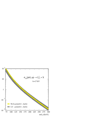
Figure 4.2: Left: The renormalization/factorization scale dependence of the total cross section for $\tilde{t}_{1}$ pair production at the Tevatron and the LHC. the maximum for the NLO cross section at the LHC is reached only for very small scales; Right: Effect of the variation of the scale on the upgraded Tevatron production cross section, as a function of the stop mass. The LO and NLO bands show the improvement of the theoretical uncertainties in the derivation of mass bounds. The SUSY scenario determining the masses is given in eq.(1.45).

The hadronic cross section is obtained from the partonic by convolution with the parton densities, eq.(2.5). The phase space integration for the Born cross section as well as for the real gluon emission is given in appendix B.1.

Scale Dependence

The dependence on the scale $\mu=\mu_{F}=\mu_{R}$ has been analyzed for the production of $\tilde{t}_{1}$ pairs both at the upgraded Tevatron and at the LHC. The hadronic cross sections include $\alpha_{s}$ and the CTEQ4 [17] parton densities consistently in LO or NLO, which also enters the definition of the $K$ factor $K=\sigma_{\rm NLO}/\sigma_{\rm LO}$. The scale dependence is shown in Fig. 4.2. The leading order dependence is monotonic and varies by about $\sim 100\%$ for scales between $m_{\tilde{t}_{\scriptscriptstyle 1}}/2$ and $2m_{\tilde{t}_{\scriptscriptstyle 1}}$. The increase for small scales results from the large value of the running QCD coupling in leading order. At next-to-leading order the variation with the scale is reduced to $\sim 30\%$. The monotonic behavior of the leading order curve is corrected in next-to-leading order, yielding a maximum value at some small scale, Fig. 4.2.

Supersymmetric Parameter Dependence

Figure 4.3: $K$ factors for diagonal stop-pair production at the upgraded Tevatron and the LHC for a sample of stop masses. Scale choice: $\mu=m_{\tilde{t}_{\scriptscriptstyle 1}}$. For a comparison of Tevatron and LHC also the LO initial-state $gg$ and $q\bar{q}$ fractions are given.

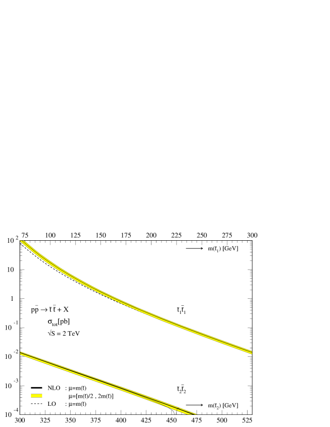
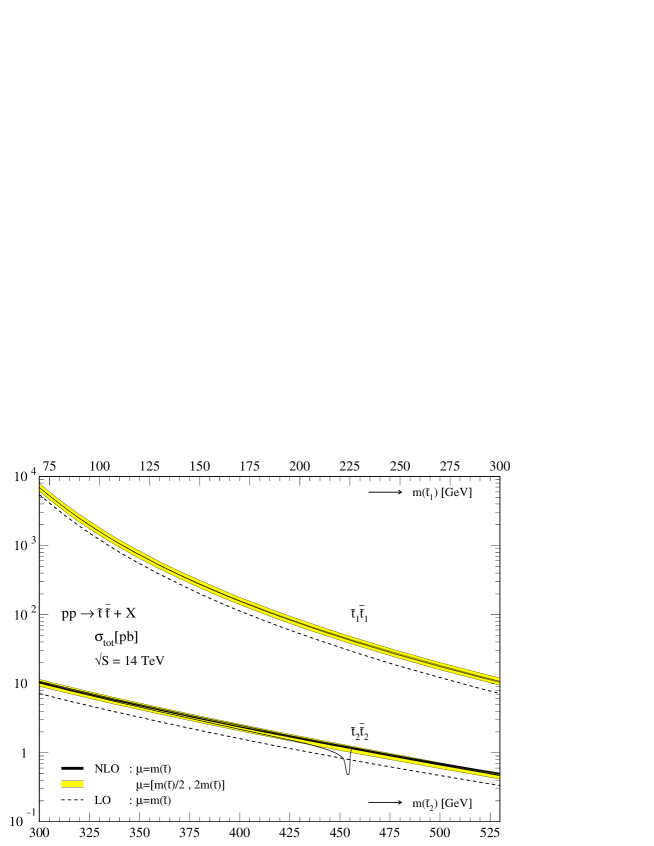
Figure 4.5: The total cross section for $\tilde{t}_{1}$ and $\tilde{t}_{2}$ pair production at the Tevatron and at the LHC. The band for the NLO results indicates the uncertainty due to the scale dependence. The mass scenario is given in eq.(1.45). The line thickness of the NLO curves represents the variation of the gluino mass between 280 and $900{\rm\,GeV}$ and of the mixing angle over its full range. The kink in both of the cross section results from the on-shell decay of the heavy stop to a very light gluino and a top, and can be regularized by introducing a finite stop width.

The total hadronic cross sections at the Tevatron and at the LHC are given in Fig. 4.5. The masses involved are fixed by a SUGRA inspired scenario eq.(1.45). All squarks except the top squark are assumed to be mass degenerate. The mass range of the outgoing stop is varied independently of the other mass parameters. The same is done for the mixing angle and for the gluino mass. The dependence of the cross section on these internal mass parameters is small, as can be seen from the finite width of the central lines in the figures, i.e. the cross sections depend essentially on the outgoing masses and do not distinguish between $\tilde{t}_{1}$ and $\tilde{t}_{2}$. The light-flavor squark and the gluino contributions appearing in the loops are decoupled even for numerically small masses. The search for stops therefore yields limits on their masses independent of any other parameter, unlike the squark/gluino or the neutralino/chargino case.

One exception of this behavior is the kink in the next-to-leading order cross sections for the heavy stops. Similarly to the decay width of a heavy stop to a gluino, Fig. 3.3, threshold contributions occur. In the stop production case the heavy stop can decay into an on-shell gluino and a top quark. The kink will be regularized by introducing a finite width for the stop, and for an analysis it has to be removed by resummation. However, for the search for stops at the Tevatron this parameter region is not of interest.

The strong mass dependence of the $K$ factor is due to different $K$ factors for the quark and the gluon channel, both of which are only weakly mass dependent. However the contribution of the two channels varies strongly with the mass of the external particle, as can be read off Fig. 4.3. Whereas the gluonic $K$ factor is large (about 1.3), the quark $K$ factor tends to be smaller than and close to one. Weighted with the fraction of the incoming state these combine to the $K$ factor given in Tab. 4.3. Since at the Tevatron the contribution of the incoming quarks decreases as the stops become light, the $K$ factor grows from 1.03 to 1.43 far from threshold. At the LHC the gluons dominate over the whole considered mass region and the $K$ factor varies between 1.27 and 1.50.

With cross sections between 0.1 and 100 pb the integrated luminosity $\int{\cal L}=20{\rm fb}^{-1}$ should be sufficient for collecting a sample of $10^{3}$ and $10^{6}$ stop events, provided the particle exists and with a mass less than $450{\rm\,GeV}$. The LHC with an integrated luminosity of $\int{\cal L}=300{\rm fb}^{-1}$ could collect $10^{5}$ to $10^{8}$ stop events in the mass range of 200 to $500{\rm\,GeV}$.

The normalized differential cross sections with respect to the transverse momentum and the rapidity is shown in Fig. 4.4. The transverse momentum of the outgoing stops is shifted to a softer regime by the momentum carried by the additional jet in the final state. A naive description using the $K$ factor would not take into account this shift and therefore lead to large errors in the size of the cross section for a certain value of $p_{T}$. The rapidity distribution keeps almost the same shape in NLO as in LO. However, it is not symmetric in NLO anymore.

4.2 Non-diagonal Stop Production

	$\sigma$[fb]	$\sigma_{q\bar{q}}$	$\sigma_{q\bar{q}}^{\rm limit}$	$\sigma_{gg}$	$\sigma_{gg}^{\rm limit}$
Tevatron	$\tilde{t}_{1}\bar{\tilde{t}}_{1}$	0.201 $\cdot 10^{3}$	0.202 $\cdot 10^{3}$	0.087 $\cdot 10^{3}$	0.087 $\cdot 10^{3}$
	$\tilde{t}_{2}\bar{\tilde{t}}_{2}$	0.333	0.337	0.016	0.016
	$\tilde{t}_{1}\bar{\tilde{t}}_{2}+\tilde{t}_{2}\bar{\tilde{t}}_{1}$	–	0	–	0.131 $\cdot 10^{-4}$
LHC	$\tilde{t}_{1}\bar{\tilde{t}}_{1}$	4.137 $\cdot 10^{3}$	4.150 $\cdot 10^{3}$	70.13 $\cdot 10^{3}$	75.00 $\cdot 10^{3}$
	$\tilde{t}_{2}\bar{\tilde{t}}_{2}$	0.169 $\cdot 10^{3}$	0.172 $\cdot 10^{3}$	1.422 $\cdot 10^{3}$	1.458 $\cdot 10^{3}$
	$\tilde{t}_{1}\bar{\tilde{t}}_{2}+\tilde{t}_{2}\bar{\tilde{t}}_{1}$	–	0	–	0.149

Table 4.1: Cross sections for diagonal and non-diagonal pair production at the Tevatron and the LHC, using the default SUGRA-inspired scenario eq.(1.45). The non-diagonal results are given without the mixing factor $\sin^{2}(4\tilde{\theta})$.The superscript ’limit’ denotes the asymptotic value of the cross section for large gluino masses.

In hadron collisions mixed pairs $\tilde{t}_{1}\bar{\tilde{t}}_{2}$ and $\tilde{t}_{2}\bar{\tilde{t}}_{1}$ cannot be produced in lowest order, unlike in $e^{+}e^{-}$ collisions, since the involved coupling conserve the chirality eigenstate, which does not hold for the coupling to a $Z$. The mixed production cross section is therefore ${\cal O}(\alpha_{s}^{4})$. For a general mass scenario it is small but difficult to calculate. In the diagonal production we observe that the limit of a decoupled gluino gives a good approximation for the size of the cross sections. Therefore we calculate the production cross section for $\tilde{t}_{1}\bar{\tilde{t}}_{2}+\tilde{t}_{2}\bar{\tilde{t}}_{1}$ in this limit. Only two one-loop diagrams contribute to the amplitude in the limit, they are given in Fig. 4.6 e. They involve the production of diagonal stop pairs in $gg$ fusion, which are rescattered to mixed pairs by the four squark vertex. The incoming quarks are suppressed.

The evaluation of the loops yields

$$\hat{\sigma}_{\infty}[gg\to\tilde{t}_{1}\bar{\tilde{t}}_{2}+\bar{\tilde{t}}_{1}\tilde{t}_{2}]=\sin^{2}(4\tilde{\theta})\,\frac{37}{13824}\,\frac{\alpha_{s}^{4}\,\Lambda^{1/2}}{2\pi s^{3}}\,\left|m_{\tilde{t}_{\scriptscriptstyle 1}}^{2}\log^{2}(x_{1})-m_{\tilde{t}_{\scriptscriptstyle 2}}^{2}\log^{2}(x_{2})\right|^{2}$$ (4.8)

where the subscript in the cross section $\hat{\sigma}_{\infty}$ indicates the limit $m_{\tilde{g}}\to\infty$. The coefficient $\Lambda^{1/2}$ is the usual 2-particle phase-space factor, i.e. $\Lambda=[s-(m_{\tilde{t}_{\scriptscriptstyle 1}}+m_{\tilde{t}_{\scriptscriptstyle 2}})^{2}][s-(m_{\tilde{t}_{\scriptscriptstyle 1}}-m_{\tilde{t}_{\scriptscriptstyle 2}})^{2}]$, and $x_{k}=(\beta_{k}-1)/(\beta_{k}+1)$; the logarithmic discontinuities are defined properly by the infinitesimal shift $s\to s+i\varepsilon$ in $\beta_{k}$. The fraction $37/13824$ originates from the color factor $(N-1)[5N^{2}-2(N-1)^{2}]/[256N^{3}(N+1)]$.

The cross section depends strongly on the mixing angle $\tilde{\theta}$ through the overall factor $\sin^{2}(4\tilde{\theta})$. Numerical values for the diagonal and non-diagonal pair cross sections are compared in Tab. 4.1. Note that the mixed-pair cross section is given in this table without the mixing factor $\sin^{2}(4\tilde{\theta})$. The values for the cross section for producing mixed stop pairs in the large $m_{\tilde{g}}$ limit are very small at the Tevatron as well as at the LHC.

Figure 4.4: The normalized differential cross section for the production of $\tilde{t}_{1}$ pairs at the Tevatron. The mass scenario using the central scale is defined in eq.(1.45).

Figure 4.6: Generic Feynman diagrams for the diagonal stop pair production: (a) Born diagrams for quark and gluon incoming state; (b) vertex corrections; (c) box contributions; (d) real gluon/quark emission for different incoming states; (e) mixed stop pair production in the limit of decoupled gluinos. The self energy contributions are not shown.

Chapter 5 $\mathbf{R}$ Parity Violating Squarks

5.1 Production in $\mathbf{ep}$ Collisions

Limits on the mass and the coupling $\lambda^{\prime}$ as defined in eq.(1.6) can be derived from the direct search at different colliders. HERA $ep$ scattering could produce squarks via the $R$ parity violating coupling $\lambda^{\prime}$ to quarks and electrons, where the flavor of the squark has to be chosen consistent with the whole set of current bounds [53, 24, 25]:

$$eq\longrightarrow\tilde{q}$$ (5.1)

This resonant $s$ channel production process can be described in terms of general scalar leptoquarks. The Yukawa matrix $\lambda^{\prime}$ does not have to be diagonal in flavor or generations.

For the leading order hadronic cross section the convolution with the parton density, as defined in eq.(2.5) becomes trivial, since the energy-momentum conservation yields a factor $\delta(1-m^{2}/(xS))$

$$\hat{\sigma}_{\rm LO}= \;\frac{\pi{\lambda^{\prime}}^{2}}{4m^{2}}$$

$$\sigma_{\rm LO}= \;\frac{m^{2}}{S}\,f^{P}_{q}\left(\frac{m^{2}}{S},\mu^{2}\right)\,\hat{\sigma}_{\rm LO}$$ (5.2)

The parton densities $f^{P}_{q}$ are taken at the factorization scale $\mu$, and possible flavors of incoming quark are fixed by charge conservation and the charge of the outgoing squark.

The NLO contributions consist of virtual gluons, real gluon emission, and the crossed $eg$ incoming state. All other supersymmetric particles in this scenario are assumed to be decoupled, see appendix A.3. Some generic Feynman diagrams for the matrix element can be derived from Fig. 3.1 by replacing the external gluino by a positron and removing all internal gluino contributions. After renormalization and mass factorization the dimensionally regularized NLO cross section is finite and can be written as

$$\sigma_{\rm NLO}= \;\frac{m^{2}}{S}\,f^{P}_{q}(x)\,\hat{\sigma}_{\rm LO}\left[1-\frac{C_{F}\alpha_{s}}{\pi}\zeta_{2}\right]+\Delta_{q}+\Delta_{g}$$

$$\Delta_{q}= \;\frac{\alpha_{s}}{\pi}\,\hat{\sigma}_{\rm LO}\int_{x}^{1}dy\,f^{P}_{q}(y)\,\Bigg{\{}-\frac{z}{2}P_{qq}(z)\log z+C_{F}\left(1+z\right)$$

$$\qquad\qquad\qquad+C_{F}\left[2\left(\frac{\log(1-z)}{1-z}\right)_{+}-\left(\frac{1}{1-z}\right)_{+}-(2+z+z^{2})\log(1-z)\right]\Bigg{\}}$$

$$\Delta_{g}= \;\frac{\alpha_{s}}{\pi}\,\hat{\sigma}_{\rm LO}\int_{x}^{1}dy\,f^{P}_{q}(y)\,\frac{z}{2}\Bigg{\{}-P_{qg}(z)\left[\log\frac{z}{(1-z)^{2}}+2\right]+z(1-z)\log z+1\Bigg{\}}$$ (5.3)

where $x=m^{2}/S$ and $z=x/y$, and the renormalization and factorization scales are set $\mu_{F}=\mu_{R}=m$. The splitting functions $P_{ij}$ are defined in eq.(B.23), and the + distributions are given in eq.(B.24). The NLO cross section is proportional to $\hat{\sigma}_{\rm LO}$, i.e. the anomalous coupling drops out of the $K$ factor. In the formulae the factorization and renormalization scales have been identified with the squark mass.

The $K$ factors for the production of an up-type and a down-type squark are given in Fig. 5.1. The next-to-leading order correction for the HERA process is dominated by the gluon emission from an incoming quark. They are positive in the whole mass region considered. The virtual correction as well as the crossed channel are suppressed. Since the parton distributions enter the $K$ factor, the different up and down type valence and sea quarks receive different corrections.

Figure 5.1: Left: $K$ factors for $ed,eu\to\tilde{q}$ as a function of the mass of the produced squark; Right: $K$ factor for the $d$ type quark vs. the renormalization and factorization scale.

The dependence on the factorization and renormalization scale can be made explicit in eq.(5.3) by adding $\log\mu_{FR}^{2}/m^{2}$ to the $\zeta_{2}$ term in the virtual correction and to the logarithms multiplied by $P_{ij}$. Additionally the mass $m$ in the argument of the parton densities and the running coupling $\lambda^{\prime}$ has to be replaced by $\mu$. The decrease of the scale dependence of the cross section is shown in Fig. 5.1.

The partial width for the decay of a $R$ parity violating squark can be computed using the results for the scalar top squark. The width for the decay channel

$$\tilde{q}\longrightarrow eq$$ (5.4)

in NLO reads

$$\Gamma_{\rm NLO}(\tilde{q}\to eq)=\frac{{\lambda^{\prime}}^{2}m}{16\pi}\left[1+\left(\frac{27}{8}-2\zeta_{2}\right)\frac{C_{F}\alpha_{s}}{\pi}\right]$$ (5.5)

This correction is small ($\sim 10\%$). If the $R$ parity breaking coupling $\lambda^{\prime}$ is small, then the squark will be long-lived, and the NLO correction will not change this effect. A typical scenario could be a squark with a mass of $200{\rm\,GeV}$ and a Yukawa coupling $\lambda^{\prime}\sim e/10$, which leads to a decay width of $\Gamma\sim 3{\rm\,GeV}$. Bound states however will only occur, if $R$ parity conserving decay modes are kinematically forbidden.

5.2 Production in Hadron Collisions

In contrast to the HERA production process the production of squarks at hadron colliders, $R$ parity conserving and $R$ parity violating, is fixed by the QCD coupling, as long as the production process does not involve any weakly interacting particles. In the scenario under consideration all other non-Standard Model particles are decoupled. The Feynman diagrams for the Born cross section [14] are the same as for the stop pair production, Fig. 4.6a:

$$q\bar{q}\,/\,gg\longrightarrow\tilde{q}\bar{\tilde{q}}$$ (5.6)

Figure 5.2: Renormalization/factorization scale dependence of the total cross section $p\bar{p}\to\tilde{q}\bar{\tilde{q}}$ at the non-upgraded Tevatron. The arrow indicated the average invariant energy $<s>^{1/2}$ in the hard subprocess, which was used in the original analysis.

The Born cross section is given by eq.(4.2), the $t$ channel diagram for quark-antiquark collisions is in this case not suppressed by the incoming state but absent, due to the decoupling of the gluino. The strong coupling is independent of the flavor of the light squark, i.e. in case of hadroproduction all flavors look identical, unlike Fig. 5.1. The calculation for $R$ parity breaking squark production is the same as for the stop pairs, the Feynman diagrams are given in Fig. 4.6 taking the limit of decoupling gluino and removing the strong four-squark coupling. This follows from appendix A. The partonic NLO cross section only depends on the partonic cm energy $s$ and on the mass of the squark, leading to the [in this case literal] scaling functions for the Born, virtual and soft, hard, and scale dependent contributions

$$\hat{\sigma}_{ij}=\frac{\alpha_{s}^{2}(\mu^{2})}{m_{\tilde{q}}^{2}}\left\{f_{ij}^{B}(\eta)+4\pi\alpha_{s}(\mu^{2})\left[f_{ij}^{V+S}(\eta)+f_{ij}^{H}(\eta)+\bar{f}_{ij}(\eta)\log\left(\frac{\mu^{2}}{m_{\tilde{q}}^{2}}\right)\right]\right\}$$ (5.7)

where $i,j$ denote the initial state partons. The factorization and the renormalization scale have been identified, and $\eta=s/(4m_{\tilde{q}}^{2})-1$. The numerical form and the structure of these scaling functions are very similar to the stop case, Fig. 4.1, since the SUSY parameters except for the outgoing mass influence the stop scaling functions only marginally, and the four-squark vertex only contributes to the numerically suppressed virtual corrections. This result for the $R$ parity violating squarks can also be obtained from the even more general light-flavor squark production [8] in the limit of a large gluino mass. However, the occurrence of the gluino mass in the Born term requires a numerically large gluino mass for the analysis. And the four-squark coupling has to be removed as for the derivation from the diagonal stop pair production.

Exactly as for the stops, the scale dependence Fig. 5.2 in NLO leads to a maximum and an increasing accuracy for the derivation of limits on the mass of the particles from non-observation. Since in leading order any scale of the process can be considered, choosing the invariant energy of the final state $\mu=\sqrt{s}$ is possible. Especially if NLO calculations are not available the choice of the scale of the process leads to considerable uncertainties, which is illustrated in this example: In NLO the choice of the factorization scale is no longer free, since it must be a parameter defined in terms of external variables, which does not allow for $\mu=\sqrt{s}$. The choice of $\mu=\sqrt{s}$ in next-to-leading order leads to an inconsistence of the order $\alpha_{s}$, independent of the order of perturbation theory, in which the process has been calculated [48]. Another scale for the production of massive particles would be the final state mass $m$, which turns out to be much smaller than $\sqrt{s}$ averaged with the weight of the cross section. The different $K$ factors for both choices of the scale are given in Fig. 5.2. For the typical behavior of the leading and next-to-leading order cross section the large scale, $\sqrt{s}$, is far from the point of maximal convergence. This reflects the appearance of logarithms $\log m^{2}/\mu^{2}$, which render the corrections unnaturally large.

The NLO cross section and the LO cross section for the central mass scale for the upgraded Tevatron are given in Fig. 5.3. The variation of the cross section with the scale decreases from $100\%$ to $30\%$ if the NLO result is used. Compared to the $\mu=m$ leading order result this leads to a more accurate and always higher mass limit, the improvement of the mass bounds however stays below $10{\rm\,GeV}$ for the central scale.

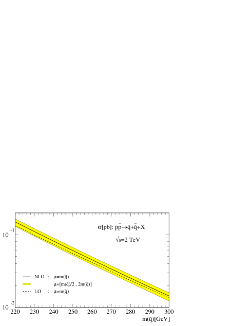
Figure 5.3: Total hadronic cross section for the production of $R$ parity violating squarks in hadron collisions $p\bar{p}\to\tilde{q}\bar{\tilde{q}}$. The leading order result is given for the renormalization/factorization scale $\mu=m$. In the first case also the values of $\alpha_{s}$ and the parton densities have been taken in leading order. The $K$ factor for the smaller central scale $m$ is comparably small.

Experimental Analyses

One of the design features of the $ep$ collider HERA is the search for leptoquark-like particles, i.e. particles which carry electron and quark quantum numbers, and can in case of scalars be identified with $R$ parity violating squarks. They can occur either in the $s$ or in the $t$ channel and lead to an excess in the $ep$ cross section [49]. The decay channel of this squark strongly depends on the masses of the supersymmetric scenario considered, but may well include a high-$p_{T}$ electron. This signal is essentially background free [23]. The interpretation of the combined data of ZEUS and H1 as $R$ parity violating squarks leads to combined limits on the Yukawa coupling $\lambda^{\prime}$ and the branching ratio ${\rm BR}$ to the observed high-$p_{T}$ electron final state [The numbers are based on the data analyzed by fall 1997.].

$$e^{+}u\quad: \qquad\lambda^{\prime}\sqrt{{\rm BR}}\sim 0.017\cdots 0.025$$

$$e^{+}d\quad: \qquad\lambda^{\prime}\sqrt{{\rm BR}}\sim 0.025\cdots 0.033$$

$$e^{+}s\quad: \qquad\lambda^{\prime}\sqrt{{\rm BR}}\sim 0.15\cdots 0.25$$ (5.8)

Couplings to $\bar{d}$ and $\bar{u}$ would lead to a large enhancement in the $e^{-}p$ run and are forbidden because of their non-observation. Moreover, couplings involving a positron and an up-type quarks would lead to electric charges, which do not occur for MSSM-type squarks. The coupling $\lambda^{\prime}$ has to be interpreted as entries into the non-diagonal Yukawa coupling matrix, connecting down-type quarks to squarks and electrons. The diagonal matrix element $\lambda^{\prime}_{111}$, which would lead to the production $e^{+}d\to\tilde{u}$, is excluded by neutrinoless double beta decay. Possible candidates for a resonance production are

$$e^{+}d\to\tilde{c}_{L},\tilde{t}_{L}\qquad\qquad\qquad e^{+}s\to\tilde{t}_{L}$$ (5.9)

As depicted in section 1.2.1, atomic parity violation yields strong limits on $\lambda^{\prime}{}^{2}/m^{2}$ for any leptoquark interacting with valence quarks. They can for a mass of $\sim 200{\rm\,GeV}$ be translated into bounds on the Yukawa coupling matrix $\lambda^{\prime}\lesssim 0.055\,[e^{+}d]$ [24, 25]. Combined with the measured values at HERA, eq.(5.8), this yields lower limits on the branching ratio to the observed $eq$ final state ${\rm BR}\gtrsim 0.2\cdots 0.4\,[e^{+}d]$. The limits obtained from atomic parity violation are derived for the presence of only one particle being responsible for the possible deviation from the Standard Model. More than one $R$ parity violating squark influences this analysis, the result depending on the sign of interference terms and thereby on the quantum numbers. The assumed left handed stop quark is in general a superposition of two states with different mass and equal electroweak properties. This strengthens the bound on the branching ratio:

$${\rm BR}\longrightarrow{\rm BR}\left(1+\tan^{2}\tilde{\theta}\,\frac{m_{\tilde{t}_{\scriptscriptstyle 1}}^{2}}{m_{\tilde{t}_{\scriptscriptstyle 2}}^{2}}\right)$$ (5.10)

At LEP, the obtained limits on $\lambda^{\prime}$ are relevant for sea quarks only [24, 25]. By the same token as for atomic parity violation they start from $\lambda^{\prime}\lesssim 0.6\,[e^{+}s]$ and give ${\rm BR}\gtrsim 0.05\cdots 0.2\,[e^{+}s]$.

The data from the search at the Tevatron can be written — given the mass of $\sim 200{\rm\,GeV}$ from the HERA analysis — as an upper bound in the branching ratio ${\rm BR}\lesssim 0.5\cdots 0.7$. Theoretically the competition between supersymmetric $R$ parity conserving, and $R$ parity violating decays makes it possible to vary the branching ratio into the $eq$ mode with the mass of the particles forming the decay chains.

In the case of $ed\to\tilde{c}_{L}$ the most important MSSM-like decay modes are $c\tilde{\chi}_{j}^{0}$ and $s\tilde{\chi}_{j}^{+}$. Assuming the gauginos being heavy [$m_{\tilde{\chi}_{\scriptscriptstyle 1}^{\scriptscriptstyle+}}>200{\rm\,GeV}$] insures that the branching ratio lies in the region of ${\rm BR}\sim 1/2$. The higgsino decays suffer from the small strange quark mass. For $ed\to\tilde{t}_{L}$ the strong decay channels are forbidden, as depicted in section 3. The decays into $t\tilde{\chi}_{j}^{0}$ and $b\tilde{\chi}_{j}^{+}$ can be suppressed by large gaugino and higgsino mass parameters. However, suppressing the whole set of possible stop decays, eq.(3.1), yields some fine tuning of masses and mixing also in the sbottom sector. The coupling $\lambda^{\prime}$ for the $es\to\tilde{t}_{L}$ production channel is comparably large, which renders the different Yukawa coupling and gauge coupling mediated decay channels of similar size, and thereby prevents from any fine tuning.

The interpretation of the HERA excess as $R$ parity violating squarks is therefore not ruled out by the bounds set by other experimental and theoretical analyses, but give an impression how different collider experiments and non-collider experiments like atomic parity violation and search for neutrinoless beta decay can altogether constrain the parameters in the same model. Incorporating all available data, HERA itself is the only experiment able to remove this interpretation by non-confirming the excess.

Chapter 6 Conclusions

In this work supersymmetric QCD corrections to decays involving scalar top quarks and to the hadroproduction of neutralinos/charginos and stops are presented. The decay widths as well as the production cross sections calculated in perturbation theory exhibit an unphysical dependence on the renormalization and/or factorization scales. In leading order this dependence is in general strong. Compared to a central scale, which could be the mass $m$ for the decay width and the hadro–production cross section of massive particles, this leads to variations up to a factor of two for scales between $m/2$ and $2m$. In next-to-leading order this dependence is considerably weaker, i.e. in addition to the $K$ factor, the next-to-leading order results always improve the precision of the theoretical prediction used for the experimental analysis.

The basic properties of the scalar top sector are investigated by calculating the supersymmetric QCD corrections to the strongly and weakly coupling decays, including a stop either in the initial or in the final state. An elegant definition of a running mixing angle in next-to-leading order is given, in order to restore the Born type symmetries between the stops in next-to-leading order observables. The mixing angle counter term is compared to other renormalization schemes. Although the phenomenological motivations for the various schemes are different, the numerical differences are shown to be small.

The different stop decay widths obey a strong hierarchy, starting with rare decay channels, and then proceeding towards weak and strong two-body decays for an increasing mass of the decaying stop. The strong decay will be dominant for a heavy stop state. The next-to-leading order corrections to the heavy stop state decaying into a gluino are large $\sim 30\%$ and always positive, while for the gluino decay into a top squark they turn out to be small and negative $\sim-5\%$. This feature also arises for the light-flavor squarks and is due to interference between different color structures and the different analytical continuation of logarithms. The dependence of all decay widths on the mixing angle can be described by a $K$ factor, which stays constant for varying angle. The scale dependence of the decay widths is reduced from a factor of two to about $50\%$ in next-to-leading order.

The weak decays of a light stop into a neutralino and a chargino are analyzed, to illustrate the running mixing angle. The next-to-leading order supersymmetric QCD corrections are small compared with typical strong decays. Apart from special mass scenarios and threshold effects they are $\lesssim 10\%$. In contrast to the strong decays the sign of the correction is not fixed, it is strongly dependent on the mass scenario considered. The same holds for decays of heavy neutralinos. They can be produced at $e^{+}e^{-}$ linear colliders and will in supergravity inspired scenarios be higgsino-like. Therefore the decay induced by the top-stop Yukawa coupling can give large contributions, whereas the light-flavor final states are strongly suppressed. The next-to-leading order corrections to these widths are moderate: $\sim 10\%$.

The next-to-leading order production cross section for neutralinos and charginos can be used to derive mass limits at the upgraded Tevatron and at the LHC. This yields an improvement of the mass bounds for these particles obtained at LEP2. Although mass and mixing parameters could be derived from cascade decays of strongly interacting particles, the only way to keep maximal independence of the choice of the model is the direct search. Similar to the case of gluino production, on-shell and off-shell intermediate particle contributions have to be distinguished. This is done in a manner, which naturally coincides with the experimental analyses. The different higgsino-like and gaugino-like contributions to the production cross section can be analyzed and give a smooth picture of the next-to-leading order corrections. Although the scale dependence in next-to-leading order is not as much improved as for strongly interacting particles, where the dependence on the running QCD coupling arises in leading order, it stays below few percent in next-to-leading order. The $K$ factor for all possible final state neutralinos/charginos is nearly constant for varying masses and corrects the leading order result by +20$\%$ to +50$\%$. However, strong cancelations between different diagrams may lead to large $K$ factors in the mixed production channel, strongly dependent on the mass and mixing parameters chosen.

The search for scalar top quarks is naturally the next step after the search for light-flavor squarks and gluinos at the upgraded Tevatron and at the LHC. Since the QCD type couplings are invariant under chiral transformations, and cannot distinguish between the right and the left stop, the production cross section in leading order depends only on the mass of the produced particles. The mixing angle as well as the mass of the light-flavor squarks and the gluino only enters through the virtual corrections. This dependence is found to be much smaller than the scale dependence and thereby negligible. The corrections to the diagonal stop pair production are different for quark and gluon incoming states. Whereas they are small and negative $\sim-5\%$ for incoming quarks, they are large and positive $\sim 50\%$ for gluons. Since even at the Tevatron only very heavy stops are produced mainly in quark-antiquark collisions, this mass dependent $K$ factor leads to an increase of the mass bounds derived in leading order. In addition to the total cross section the differential cross sections are analyzed: The rapidity distribution at the upgraded Tevatron can be described using a $K$ factor, the transverse momentum distribution however is shifted to a softer regime in next-to-leading order.

The search for mixed stop final states could be a means to measure the stop mixing angle directly at hadron colliders. However, the cross section is based on a one-loop amplitude, and the calculation in the limit of decoupled gluinos shows, that it is much smaller than the cross section for the production of two heavy stop particles. The direct measurement of the stop mixing angle will be possible only in the process $e^{+}e^{-}\to\tilde{t}_{1}\bar{\tilde{t}}_{2}$.

The calculation of the stop production cross section can be adapted to the search for supersymmetric $R$ parity violating squarks at the Tevatron. Similar to the HERA production process, the next-to-leading order calculation for the hadroproduction gives rise to improved bounds on the mass and on the branching ratio into the observed $eq$ channel. However, this is not sufficient to close the window in the branching ratio between the atomic parity violation and LEP on one side and the Tevatron on the other side, before the excess completely vanishes by accumulating more HERA data.

All calculations have been performed in a supergravity inspired GUT scenario. This connects not only the different gaugino masses, but also the masses of the squarks and the stops. All these particles can be searched for at the upgraded Tevatron and at the LHC. In Fig. 6.1 the relevant cross sections are given as a function of the mass of the produced particles. The weakly interacting particles are strongly suppressed at the LHC; however, the search for leptonic events at hadron colliders is completely different from the hadronic final states. Assuming a similar efficiency for the search for stops and light-flavor squarks the search for both of them in parallel seems to be promising, in particular, since the search for squarks is a two dimensional, the search for stops a one dimensional problem. The smaller stop cross section, due to the missing $t$ channel gluino contribution and the fixed non-degenerate flavor, is compensated by the small mass of the light stop state in typical scenarios. For gluinos, like-sign leptons in the final state should improve the efficiency considerably, yielding all production processes given in Fig. 6.1 very promising at the upgraded Tevatron and the LHC.

Figure 6.1: The total cross section for pairs of squarks, gluinos, stops, and neutralinos/charginos as a function of the mass of the produced particles. The usual SUGRA mass spectrum $m_{0}=100{\rm\,GeV},m_{1/2}=150{\rm\,GeV},A_{0}=300{\rm\,GeV},\tan\beta=4,\mu>0$ is denoted by the arrows. The masses of $\tilde{\chi}_{2}^{0}$ and $\tilde{\chi}_{1}^{-}$ differ only by a few ${\rm\,GeV}$ in the small $m_{1/2}$ regime. For the neutralino/chargino production cross section the masses are consistently varied with $m_{1/2}$. The cross sections are given for the upgraded Tevatron and for the LHC.

Acknowledgments

I would like to thank my advisor, Prof. Peter M. Zerwas, for the continuous support of this work and for his enthusiasm and encouragement.

Furthermore, I would like to thank Roland Höpker, Wim Beenakker and Michael Krämer for a pleasing collaboration and encouraging discussions. Also I would like to thank Michael Spira for his guidance and countless clarifying discussions during our collaboration in the last five years.

Finally I would like to thank Michael Plümacher, Gudrun Hiller, Thomas Gehrmann, Aude Gehrmann-De Ridder, Axel Krause, Hubert Spiesberger, Christoph Jünger, and all members of the DESY theory group for numerous discussions and an enjoyable working atmosphere.

Appendix A SUSY Lagrangean

A.1 Feynman Rules for Supersymmetric QCD

In this appendix we give a complete set of Feynman rules, as used in the calculation of the various processes. Since fermion number violating processes have to be considered, the rules make use of a continuous fermion flow [50], which has to be fixed once for any process. The Dirac trace has to be evaluated in the opposite direction of this fermion flow. If not stated otherwise, we assume the fermion flow being identical to the Dirac fermion flow e.g. for the quarks.

Using these Feynman rules makes it needless to introduce charge conjugation matrices. Moreover, the relative signs of different diagrams contributing to the same process can be fixed: Any permutation of the fermion flow of two external fermion lines gives rise to a factor $(-1)$ for the matrix element, due to Fermi statistics and Wick ordering. To match the spinors for processes including two external Majorana and two external Dirac fermions, all diagrams have to be evaluated with two different directions of the fermion flow. We have checked explicitly that the two possible orientations of the fermion flow of two combined diagrams lead to the same result.

By changing the orientation of the fermion flow, the signs of vertices with different types of couplings [$S,P,V,A$] change:

coupling			sign
scalar ($S$)	$C\;1\;C^{-1}\;=$	$1^{T}$	$+$
pseudo-scalar ($P$)	$C\;\gamma_{5}\;C^{-1}\;=$	$\gamma_{5}^{T}$	$+$
vector ($V$)	$C\;\gamma_{\mu}\;C^{-1}\;=$	$-\gamma_{\mu}^{T}$	$-$
axial-vector ($A$)	$C\;(\gamma_{5}\gamma_{\mu})\;C^{-1}\;=$	$(\gamma_{5}\gamma_{\mu})^{T}$	$+$

Table A.1: Transformation of couplings with the orientation of the fermion flow. $C$ is the charge conjugation matrix.

Standard Model Feynman Rules

All momenta in the Feynman rules are defined incoming. The Standard Model couplings of quarks, gluons, Fadeev-Popov ghosts and weak gauge bosons are given in Fig. A.1 in the Feynman gauge. The generators of SU(3)_C obey the relations

$${\rm Tr}\left(T^{a}T^{b}\right)=\frac{1}{2}\delta^{ab}\qquad\qquad\left[T^{a},T^{b}\right]=if^{abc}T_{c}$$ (A.1)

Figure A.1: Feynman rules for Standard Model quarks, gluons, ghosts and weak gauge bosons, the dotted lines for scalars refer to Fadeev-Popov ghosts. The generic couplings $\ell,r$ are defined in Tab. A.2; $P_{LR}$ are the chiral projectors $(1\mp\gamma_{5})/2$

	$\ell$	$r$
$q\bar{q}\gamma$	$Qe$	$\ell$
$q\bar{q}Z$	$\displaystyle\frac{e}{s_{w}c_{w}}\left(T_{3}-Qs_{w}^{2}\right)$	$\ell\;[T_{3}=0]$
$u\bar{d}W^{+}_{\rm out}$	$\displaystyle\frac{e}{\sqrt{2}s_{w}}$	0

Table A.2: Couplings of quarks to weak gauge bosons as used in Fig. A.1.

The fermion propagators are defined as $i/(\hbox to0.0pt{\hbox{$\mskip 1.0mu/$}\hss}p-m+i\varepsilon)$, where $p$ is the momentum in the direction of the fermion flow. The fermion number flow does not occur. The gluon propagator is $-ig^{\mu\nu}/(p^{2}+i\varepsilon)$.

Supersymmetric QCD Feynman Rules

The Feynman rules for supersymmetric QCD include, besides the Standard Model particles, the gluino ($\tilde{g}$), the light flavor squarks ($\tilde{q}_{\scriptscriptstyle L},\tilde{q}_{\scriptscriptstyle R}$), and the mixing top squarks ($\tilde{t}_{1},\tilde{t}_{2}$). Like in Fig. A.1, all momenta are defined incoming. The coupling $q\tilde{q}\tilde{g}$ preserves the helicity of the quark and its scalar partner as well as the flavor. In higher orders it has to be modified to restore the supersymmetric Ward identity, as described in chapter 1.5. The same holds for the $\tilde{q}\tilde{q}g$ coupling. In leading order we use $g_{s}$ for all strong Standard Model and their supersymmetry transformed couplings.

Figure A.2: Feynman rules for supersymmetric QCD. The dotted lines denote the squark $\tilde{q}_{\scriptscriptstyle L},\tilde{q}_{\scriptscriptstyle R}$. The tensors $S_{ijkl}$ are defined in Tab. A.3; $P_{LR}$ are the chiral projectors $(1\mp\gamma_{5})/2$

The $\tilde{q}\tilde{q}g(g)$ vertices preserve the flavor and the ’helicity’ of the squark. Since only two squarks are present, this coupling cannot mix the mass eigenstates.

The $q\tilde{q}\tilde{g}$ vertex Feynman rule is given for a light-flavor $\tilde{q}_{\scriptscriptstyle LR}$ with the corresponding sign and projector. To obtain the rules for $\tilde{t}_{1}$ one has to add the contributions of the helicity eigenstates and multiply the $L$ term with $\sin\tilde{\theta}$ and the $R$ term with $\cos\tilde{\theta}$. The mixing of the scalar top quark is described in detail in chapter 1.2.4. The relevant terms for stop mixing in the Lagrangean include the coupling to the gluino and the four squark coupling which arises from the $D$ term in the scalar potential, described in eq.(1.4). They can be expressed using the permutation operator

$${\cal P}_{12}\quad:\quad[\tilde{t}_{1}\leftrightarrow\tilde{t}_{2};\ c_{\tilde{\theta}}\to-s_{\tilde{\theta}},\ s_{\tilde{\theta}}\to c_{\tilde{\theta}}]$$ (A.2)

which links the vertices including $\tilde{t}_{1}$ and $\tilde{t}_{2}$

$${\cal L}_{3}\quad =\ -\sqrt{2}\,g_{s}T^{a}_{ij}\left(1+{\cal P}_{12}\right)\bar{\tilde{g}}_{a}\Big{[}c_{\tilde{\theta}}\,P_{L}-s_{\tilde{\theta}}\,P_{R}\Big{]}t_{j}\,\tilde{t}_{1}{}_{i}^{*}+\text{h.c.}$$

$${\cal L}_{4}\quad =\ -\frac{g_{s}^{2}}{8}\,\left(1+{\cal P}_{12}\right)\tilde{t}_{1}{}_{i}^{*}\,\tilde{t}_{1}{}_{j}\,\bigg{\{}c^{2}_{2\tilde{\theta}}\,S_{2}^{ijkl}\,\tilde{t}_{1}{}_{k}^{*}\,\tilde{t}_{1}{}_{l}+2\,\Big{[}s^{2}_{2\tilde{\theta}}\,S_{2}^{ijkl}-S_{1}^{ijkl}\Big{]}\,\tilde{t}_{2}{}_{k}^{*}\,\tilde{t}_{2}{}_{l}$$

$$\hphantom{-\frac{g_{s}^{2}}{8}\,\left(1+{\cal P}_{12}\right)\tilde{t}_{1}{}_{i}^{*}\,\tilde{t}_{1}{}_{j}aA}{}+4\,c_{2\tilde{\theta}}\,S_{1}^{ijkl}\sum_{\tilde{q}\neq\tilde{t}}\big{(}\tilde{q}_{\scriptscriptstyle L}{}_{k}^{*}\,\tilde{q}_{\scriptscriptstyle L}{}_{l}-\tilde{q}_{\scriptscriptstyle R}{}_{k}^{*}\,\tilde{q}_{\scriptscriptstyle R}{}_{l}\big{)}\bigg{\}}$$ (A.3)

The sine/cosine of an angle $\beta$ is as usually denoted by $s_{\beta},c_{\beta}$. However, these vertices describe only processes which are essentially diagonal either in $\tilde{t}_{1}$ or in $\tilde{t}_{2}$. Four squark vertices, mixing $\tilde{t}_{1}$ and $\tilde{t}_{2}$, can be derived from the Lagrangean

$${\cal L}^{\prime}_{4}\quad =\ \frac{g_{s}^{2}}{4}\,s_{2\tilde{\theta}}\,\big{(}\tilde{t}_{1}{}_{i}^{*}\,\tilde{t}_{2}{}_{j}+\tilde{t}_{2}{}_{i}^{*}\,\tilde{t}_{1}{}_{j}\big{)}\,\bigg{\{}c_{2\tilde{\theta}}\,S_{2}^{ijkl}\,\big{(}\tilde{t}_{1}{}_{k}^{*}\,\tilde{t}_{1}{}_{l}-\tilde{t}_{2}{}_{k}^{*}\,\tilde{t}_{2}{}_{l}\big{)}$$

$$\hphantom{\frac{g_{s}^{2}}{4}\,s_{2\tilde{\theta}}\,\big{(}\tilde{t}_{1}{}_{i}^{*}\,\tilde{t}_{2}{}_{j}+\tilde{t}_{2}{}_{i}^{*}\,\tilde{t}_{1}{}_{j}\big{)}\,A}{}+2\,S_{1}^{ijkl}\sum_{\tilde{q}\neq\tilde{t}}\big{(}\tilde{q}_{\scriptscriptstyle L}{}_{k}^{*}\,\tilde{q}_{\scriptscriptstyle L}{}_{l}-\tilde{q}_{\scriptscriptstyle R}{}_{k}^{*}\,\tilde{q}_{\scriptscriptstyle R}{}_{l}\big{)}\bigg{\}}$$ (A.4)

The structure of the four squark coupling is given in terms of the flavor $f_{j}$ and the helicity of the Standard Model partner $h_{j}$. The two tensors used in Tab. A.3 are

$$S_{ijkl}^{(1)}=\left(\delta_{il}\delta_{jk}-\frac{1}{N}\delta_{ij}\delta_{kl}\right)$$

$$S_{ijkl}^{(2)}=\frac{N-1}{N}\left(\delta_{il}\delta_{jk}+\delta_{ij}\delta_{kl}\right)\phantom{HHHHAAAASSSSSSS}$$ (A.5)

$\tilde{q}_{i}\tilde{q}_{j}\tilde{q}_{k}\tilde{q}_{l}$	$S_{ijkl}$
$\tilde{q}\tilde{q}\tilde{q}\tilde{q}\quad[h_{i}=h_{j}\;h_{j}=h_{l}\;f_{i}=f_{j}\;f_{j}=f_{l}]$	$-S_{ijkl}^{(2)}$
$\tilde{q}\tilde{q}\tilde{q}\tilde{q}\quad[h_{i}=h_{j}\;h_{j}=h_{l}\;f_{i}\neq f_{j}\;f_{j}\neq f_{l}]$	$-S_{ijkl}^{(1)}$
$\tilde{q}\tilde{q}\tilde{q}\tilde{q}\quad[h_{i}\neq h_{j}\;h_{j}\neq h_{l}]$	$+S_{ijkl}^{(1)}$
$\tilde{t}_{1}\tilde{t}_{1}\tilde{q}_{\scriptscriptstyle LR}\tilde{q}_{\scriptscriptstyle LR}$	$\mp c_{2\tilde{\theta}}\;S_{ijkl}^{(1)}$
$\tilde{t}_{2}\tilde{t}_{2}\tilde{q}_{\scriptscriptstyle LR}\tilde{q}_{\scriptscriptstyle LR}$	$\pm c_{2\tilde{\theta}}\;S_{ijkl}^{(1)}$
$\tilde{t}_{1}\tilde{t}_{2}\tilde{q}_{\scriptscriptstyle LR}\tilde{q}_{\scriptscriptstyle LR}\quad\tilde{t}_{2}\tilde{t}_{1}\tilde{q}_{\scriptscriptstyle LR}\tilde{q}_{\scriptscriptstyle LR}$	$\pm s_{2\tilde{\theta}}\;S_{ijkl}^{(1)}$
$\tilde{t}_{1}\tilde{t}_{1}\tilde{t}_{1}\tilde{t}_{1}\qquad\;\;\tilde{t}_{2}\tilde{t}_{2}\tilde{t}_{2}\tilde{t}_{2}$	$-c_{2\tilde{\theta}}^{2}\;S_{ijkl}^{(2)}$
$\tilde{t}_{1}\tilde{t}_{1}\tilde{t}_{1}\tilde{t}_{2}\qquad\;\;\tilde{t}_{1}\tilde{t}_{1}\tilde{t}_{2}\tilde{t}_{1}$	$+s_{2\tilde{\theta}}c_{2\tilde{\theta}}\;S_{ijkl}^{(2)}$
$\tilde{t}_{2}\tilde{t}_{2}\tilde{t}_{2}\tilde{t}_{1}\qquad\;\;\tilde{t}_{2}\tilde{t}_{2}\tilde{t}_{1}\tilde{t}_{2}$	$-s_{2\tilde{\theta}}c_{2\tilde{\theta}}\;S_{ijkl}^{(2)}$
$\tilde{t}_{1}\tilde{t}_{1}\tilde{t}_{2}\tilde{t}_{2}$	$S_{ijkl}^{(1)}-s_{2\tilde{\theta}}^{2}\;S_{ijkl}^{(2)}$
$\tilde{t}_{1}\tilde{t}_{2}\tilde{t}_{1}\tilde{t}_{2}\qquad\;\;\tilde{t}_{2}\tilde{t}_{1}\tilde{t}_{2}\tilde{t}_{1}$	$-s_{2\tilde{\theta}}^{2}\;S_{ijkl}^{(2)}$

Table A.3: Tensors arising in the generic four squark coupling in Fig. A.2. The tensors $S^{(1)}$ and $S^{(2)}$ are defined in eq.(A.5).

A.2 Neutralinos and Charginos

Diagonalization for Neutralinos

The diagonalization procedure for Neutralinos is described e.g. in [51]. The four Majorana neutralinos ($\tilde{\chi}_{j}^{0}$) are defined as the mass basis of all neutral higgsinos, the photino, and the zino interaction eigenstates. They are four component Majorana spinors, therefore the mass matrix is symmetric. It is possible to start from a non-diagonal matrix in the $(\tilde{B}\tilde{W}_{3})$ basis or in the $(\tilde{\gamma}\tilde{Z})$ basis. We denote the two possible mass matrices as ${\cal M}$ and ${\cal M}^{\prime}$ for the two component states:

$${\cal M}=\left(\begin{array}[]{cccc}m_{\scriptscriptstyle{\tilde{B}}}&0&-m_{\scriptscriptstyle Z}s_{w}c_{\beta}&m_{\scriptscriptstyle Z}s_{w}s_{\beta}\\ 0&m_{\scriptscriptstyle{\tilde{W}}}&m_{\scriptscriptstyle Z}c_{w}c_{\beta}&-m_{\scriptscriptstyle Z}c_{w}s_{\beta}\\ -m_{\scriptscriptstyle Z}s_{w}c_{\beta}&m_{\scriptscriptstyle Z}c_{w}c_{\beta}&0&-\mu\\ m_{\scriptscriptstyle Z}s_{w}s_{\beta}&-m_{\scriptscriptstyle Z}c_{w}s_{\beta}&-\mu&0\end{array}\right)$$ (A.10)

Figure A.3: Feynman rules for neutralinos and charginos. The dotted lines denote a left or right scalar quarks $\tilde{q}_{\scriptscriptstyle L},\tilde{q}_{\scriptscriptstyle R}$. $L,R$ are defined in Tab. A.4, $A,B$ in Tab. A.5. Note that the $q\tilde{q}\tilde{\chi}$ vertices for incoming and outgoing squarks are linked.

The corresponding unitary mixing matrices $N,N^{\prime}$ diagonalize these mass matrices, $N$ in the $(\tilde{B}\tilde{W}_{3})$ and $N^{\prime}$ in the $(\tilde{\gamma}\tilde{Z})$ basis. In case the mass matrix is real, the mixing matrices $N,N^{\prime}$ are also chosen to be real, to keep the couplings from becoming complex i.e. in this special case the in general complex unitary transformation becomes real and orthogonal. However, for CP invariant observables the typical coupling factors must be purely real or imaginary for any complex unitary mixing matrix.

$$N^{*}\;{\cal M}\;N^{-1}={\cal M}_{\rm diag}$$

$$N^{\prime}{}^{*}\;{\cal M}^{\prime}\;N^{\prime}{}^{-1}={\cal M}_{\rm diag}\qquad\qquad\qquad {N^{\prime}}_{j1}=N_{j1}c_{w}+N_{j2}s_{w}$$

$${N^{\prime}}_{j2}=-N_{j1}s_{w}+N_{j2}c_{w}$$

$${N^{\prime}}_{j3}=N_{j3}$$

$${N^{\prime}}_{j4}=N_{j4}$$ (A.11)

The mixing matrix is defined in terms of the arbitrary-sign eigenvalues of the mass matrix, $m_{i}$:

$$\frac{N_{i2}}{N_{i1}}= \,-\frac{c_{w}}{s_{w}}\frac{m_{\scriptscriptstyle{\tilde{B}}}-m_{i}}{m_{\scriptscriptstyle{\tilde{W}}}-m_{i}}$$

$$\frac{N_{i3}}{N_{i1}}= \,\frac{\mu(m_{\scriptscriptstyle{\tilde{B}}}-m_{i})(m_{\scriptscriptstyle{\tilde{W}}}-m_{i})-m_{\scriptscriptstyle Z}^{2}s_{\beta}c_{\beta}[(m_{\scriptscriptstyle{\tilde{B}}}-m_{\scriptscriptstyle{\tilde{W}}})c_{w}^{2}+m_{\scriptscriptstyle{\tilde{W}}}-m_{i}]}{m_{\scriptscriptstyle Z}s_{w}(m_{\scriptscriptstyle{\tilde{W}}}-m_{i})(\mu c_{\beta}+m_{i}s_{\beta})}$$

$$\frac{N_{i4}}{N_{i1}}= \,\frac{-m_{i}(m_{\scriptscriptstyle{\tilde{B}}}-m_{i})(m_{\scriptscriptstyle{\tilde{W}}}-m_{i})-m_{\scriptscriptstyle Z}^{2}c_{\beta}^{2}[(m_{\scriptscriptstyle{\tilde{B}}}-m_{\scriptscriptstyle{\tilde{W}}})c_{w}^{2}+m_{\scriptscriptstyle{\tilde{W}}}-m_{i}]}{m_{\scriptscriptstyle Z}s_{w}(m_{\scriptscriptstyle{\tilde{W}}}-m_{i})(\mu c_{\beta}+m_{i}s_{\beta})}$$

$$N_{i1}= \,\left[1+\left(\frac{N_{i2}}{N_{i1}}\right)^{2}+\left(\frac{N_{i3}}{N_{i1}}\right)^{2}+\left(\frac{N_{i4}}{N_{i1}}\right)^{2}\right]^{-1/2}$$ (A.12)

	$L$	$R$
$\tilde{\chi}_{i}^{0}\tilde{\chi}_{j}^{0}Z$	$\displaystyle\frac{e}{2s_{w}c_{w}}\left({\mathfrak{N}^{\prime}}_{i3}{\mathfrak{N}^{\prime}}^{*}_{j3}-{\mathfrak{N}^{\prime}}_{i4}{\mathfrak{N}^{\prime}}^{*}_{j4}\right)$	$L^{*}\;[{\mathfrak{N}^{\prime}}_{k4}\leftrightarrow-{\mathfrak{N}^{\prime}}_{k3}]$
$\tilde{\chi}_{i}^{+}\tilde{\chi}_{j}^{-}\gamma$	$e\delta_{ij}$	$L^{*}$
$\tilde{\chi}_{i}^{+}\tilde{\chi}_{j}^{-}Z$	$\displaystyle\frac{e}{s_{w}c_{w}}\left(V_{i1}V^{*}_{j1}+\frac{1}{2}V_{i2}V^{*}_{j2}-\delta_{ij}s_{w}^{2}\right)$	$L^{*}\;[V\to U]$
$\tilde{\chi}_{i}^{0}\tilde{\chi}_{j}^{+}W^{+}_{\rm out}$	$\displaystyle\frac{e}{\sqrt{2}s_{w}}\left({\mathfrak{N}^{\prime}}_{i4}V^{*}_{j2}-\sqrt{2}\left(s_{w}{\mathfrak{N}^{\prime}}_{i1}+c_{w}{\mathfrak{N}^{\prime}}_{i2}\right)V^{*}_{j1}\right)$	$L^{*}\;[V\to U,{\mathfrak{N}^{\prime}}_{i4}\to-{\mathfrak{N}^{\prime}}_{i3}]$
$\tilde{\chi}_{i}^{0}\tilde{\chi}_{j}^{-}W^{+}_{\rm in}$	$\displaystyle\frac{e}{\sqrt{2}s_{w}}\left({\mathfrak{N}^{\prime}}^{*}_{i4}V_{j2}-\sqrt{2}\left(s_{w}{\mathfrak{N}^{\prime}}^{*}_{i1}+c_{w}{\mathfrak{N}^{\prime}}^{*}_{i2}\right)V_{j1}\right)$	$L^{*}\;[V\to U,{\mathfrak{N}^{\prime}}_{i4}\to-{\mathfrak{N}^{\prime}}_{i3}]$

Table A.4: Couplings of neutralinos and charginos to weak gauge bosons as used in Fig. A.3. The mixing matrix ${\mathfrak{N}^{\prime}}$ is defined in the photino-zino basis. For charginos, the fermion flow is assumed to follow the $\tilde{\chi}_{i}^{+}$ fermion number flow.

The entries of ${\cal M}_{\rm diag}$ are not necessarily positive, if the mixing matrix is kept real, i.e. the eigenvalues are only equal to the physical masses $m_{\tilde{\chi}_{\scriptscriptstyle j}}$ up to a sign. It is possible to work with a Lagrangean including negative mass eigenvalues $m_{j}$. In the final expression these eigenvalues have to be substituted by their absolute values $m_{j}\to\pm m_{\tilde{\chi}_{\scriptscriptstyle j}}$, in order to express the analytical result in terms of physical masses. An equivalent way of introducing these phases is to define a complex mixing matrix [${\mathfrak{N}},{\mathfrak{N}^{\prime}}$], in which a row is multiplied by $i$, if the corresponding eigenvalue is negative:

$$N_{kl}=\begin{cases}{\mathfrak{N}}_{kl}\quad[l=1,...,4]&\text{if eigenvalue $m_{k}$ positive}\\[2.84526pt] i{\mathfrak{N}}_{kl}\quad[l=1,...,4]&\text{if eigenvalue $m_{k}$ negative}\\ \end{cases}$$ (A.13)

The re-definition of $N^{\prime}\to{\mathfrak{N}^{\prime}}$ is defined in analogy; in typical scenarios one of the higgsino eigenvalues $m_{k}\;[k=3,4]$ turns out to be negative, whereas the re-rotation ${\mathfrak{N}}\to{\mathfrak{N}^{\prime}}$ only affects the gaugino part of the mass matrix. Using this matrix ${\mathfrak{N}},{\mathfrak{N}^{\prime}}$ one can always stick to the positive mass values.

$${\mathfrak{N}}^{*}\;{\cal M}\;{\mathfrak{N}}^{-1} =\;{\rm Diag}\left(m_{\tilde{\chi}_{\scriptscriptstyle j}}\right)$$

$${\mathfrak{N}^{\prime}}^{*}\;{\cal M}^{\prime}\;{\mathfrak{N}^{\prime}}^{-1} =\;{\rm Diag}\left(m_{\tilde{\chi}_{\scriptscriptstyle j}}\right)\qquad j=1,2,3,4$$ (A.14)

The masses of the four neutralinos are re-ordered by their size after diagonalization, where $\tilde{\chi}_{1}^{0}$ is defined being the lightest of the four. Combining the complex couplings including the matrix ${\mathfrak{N}},{\mathfrak{N}^{\prime}}$ leads to exactly the same analytical results for CP invariant observables as using the matrix $N,N^{\prime}$; the phase factors from the negative masses now enter by collecting factors of $i^{2}$ in the typical combinations of the couplings and by anti-commuting the Dirac matrices. One advantage of the latter strategy is, that the neutralino mass matrix is not fixed to real values by first principles [52].

Diagonalization for Charginos

Charginos ($\tilde{\chi}_{j}^{-},\tilde{\chi}_{j}^{+}$) are the mass eigenstates of charged winos and higgsinos. The positive and negative charge particles mix independently. Since the charginos are no Majorana particles the mass matrix is not symmetric. Nevertheless the Dirac-chargino vertices can be fermion number violating.

$${\cal M}=\left(\begin{array}[]{cc}m_{\scriptscriptstyle{\tilde{W}}}&\sqrt{2}m_{\scriptscriptstyle W}s_{\beta}\\ \sqrt{2}m_{\scriptscriptstyle W}c_{\beta}&\mu\end{array}\right)$$ (A.17)

The unitary diagonalization matrices for the positive and negative winos and higgsinos are $V$ and $U$, and the eigenvalues of the diagonalized mass matrix can in general assumed to be real. The mixing matrices themselves are only real, if $\mu$ is chosen to be real.

$$U^{*}\;{\cal M}\;V^{-1}={\rm Diag}\left(m_{\tilde{\chi}_{\scriptscriptstyle j}}\right)\qquad j=1,2$$ (A.18)

Neutralino/Chargino Feynman Rules

The Feynman rules for the neutralinos and charginos are given in Fig. A.3. The $\tilde{q}q\tilde{\chi}$ vertex is given for left and right squarks, the coupling to the mixing scalar top quark is a superposition of both couplings, as it is for the gluino case.

	$A_{L}$	$A_{R}$	$B_{L}$	$B_{R}$
$\tilde{u}u\tilde{\chi}_{j}^{0}$	$\displaystyle gs_{w}Q{\mathfrak{N}^{\prime}}_{j1}+\frac{g}{c_{w}}{\mathfrak{N}^{\prime}}_{j2}\left(T_{3}-Qs_{w}^{2}\right)$	$A_{L}^{*}\;[T_{3}=0]$	$\displaystyle\frac{gm_{u}}{2m_{\scriptscriptstyle W}s_{\beta}}{\mathfrak{N}^{\prime}}^{*}_{j4}$	$B_{L}^{*}$
$\tilde{d}d\tilde{\chi}_{j}^{0}$	$\displaystyle gs_{w}Q{\mathfrak{N}^{\prime}}_{j1}+\frac{g}{c_{w}}{\mathfrak{N}^{\prime}}_{j2}\left(T_{3}-Qs_{w}^{2}\right)$	$A_{L}^{*}\;[T_{3}=0]$	$\displaystyle\frac{gm_{d}}{2m_{\scriptscriptstyle W}c_{\beta}}{\mathfrak{N}^{\prime}}^{*}_{j3}$	$B_{L}^{*}$
$\tilde{d}u\left(\tilde{\chi}_{j}^{-}\right)_{\rm out}$	$\displaystyle\frac{g}{\sqrt{2}}U_{j1}$	$0$	$\displaystyle-\frac{gm_{u}}{2m_{\scriptscriptstyle W}s_{\beta}}V^{*}_{j2}$	$\displaystyle-\frac{gm_{d}}{2m_{\scriptscriptstyle W}c_{\beta}}U_{j2}$
$\tilde{u}d\left(\tilde{\chi}_{j}^{+}\right)_{\rm out}$	$\displaystyle\frac{g}{\sqrt{2}}V_{j1}$	$0$	$\displaystyle-\frac{gm_{d}}{2m_{\scriptscriptstyle W}c_{\beta}}U^{*}_{j2}$	$\displaystyle-\frac{gm_{u}}{2m_{\scriptscriptstyle W}s_{\beta}}V_{j2}$

Table A.5: Couplings of neutralinos and charginos to squarks and quarks as used in Fig. A.3. The mixing matrix ${\mathfrak{N}^{\prime}}$ is defined in the photino-zino basis..

A.3 $\mathbf{R}$ Parity breaking Squarks

The breaking of $R$ parity only adds new interaction terms to the Lagrangean, eq.(1.6), which are not related to any of the Standard Model gauge symmetries. For any of these scenarios including non-MSSM squark couplings, the QCD Feynman rules are still completely fixed by the requirement, that any squark should be part of the fundamental representation of SU(3)_C, i.e. carries quark-type color charge [53].

Under the simplifying assumption of one light squark flavor, one can integrate out all heavy strongly interacting supersymmetric particles and regard the $R$ parity violating scenario as the extension of the Standard Model by one leptoquark-like squark. Another difference between a scalar leptoquark model and the MSSM squark sector occurs: The MSSM four-squark coupling originates from the $D$ terms in the scalar potential eq.(1.4). In the most general effective model this term need not be present. The four-squark coupling will then be proportional to the weak coupling constant, and quadratic divergences of scalar masses occur.

The coupling to any pair of Dirac and Majorana fermions can be identified with the most general parameterization of the $\tilde{t}_{1}t\tilde{\chi}_{j}^{0}$ coupling. However, the $q\tilde{q}e$ coupling constant is not fixed by any gauge coupling, but results from the superpotential term eq.(1.6)

$${\cal L}_{\rm int}=\lambda^{\prime}\bar{e}q\tilde{q}+{\rm h.c.}$$ (A.19)

Since its Dirac structure is fixed by the helicity of the quark and the electron, the coupling can be parameterized as $-i(A_{L}P_{l}+A_{R}P_{R})$. For unpolarized particles this yields $(A_{L}^{2}+A_{R}^{2})$ in the HERA production cross section and the decay width, likewise for leading and next-to-leading order, this means the coupling completely drops out of the next-to-leading order QCD $K$ factors.

Because the coupling $\lambda^{\prime}$ connects two strongly interacting particles, it has to be renormalized, e.g. in $\overline{{\rm MS}}$. Furthermore, it runs in complete analogy to the running QCD coupling constant

$${\lambda^{\prime}}^{2}(\mu_{R})=\frac{{\lambda^{\prime}}^{2}(M)}{1+\frac{\alpha_{s}}{\pi}\log\frac{\mu_{R}^{2}}{M^{2}}}$$ (A.20)

Appendix B Radiative Corrections

B.1 Phase Space and Partonic Cross Sections

$\mathbf{(2\to 1)}$ Production Cross Section

Assume the production of one final state particle in NLO

$$q(k_{1})+\bar{q}(k_{2})\to X_{1}(p_{1})[+g(k_{3})]$$ (B.1)

with massless partons $k_{j}[j=1,2,3]$ and a massive particle in the final state $p_{1}^{2}=m^{2}$. The invariants are the usual Mandelstam variables

$$s=2(k_{1}k_{2})\qquad t_{1}=2(k_{1}k_{3})\qquad u_{1}=2(k_{2}k_{3})$$ (B.2)

These Mandelstam variables can be expressed in terms of the rescaled gluon emission angle $\theta$

$$y= \;\frac{1}{2}\left(1+c_{\theta}\right)\in[0,1]$$

$$t= \;-s(1-\tau)y$$

$$u= \;-s(1-\tau)(1-y)$$ (B.3)

where $\tau=m^{2}/s$ and $c_{\theta}=\cos\theta$. The formula for the cross section becomes [54]:

$$s\frac{d\hat{\sigma}^{R}}{dy}=K_{ij}\frac{\pi(4\pi)^{-2+\epsilon}}{\Gamma(1-\epsilon)}\left(\frac{m^{2}}{\mu^{2}}\right)^{-\epsilon}\frac{\tau^{\epsilon}(1-\tau)^{1-2\epsilon}}{y^{\epsilon}(1-y)^{\epsilon}}\sum\left|{\cal M}^{R}\right|^{2}$$ (B.4)

$K_{ij}$ are the spin-color averaging factors, for the HERA process $K_{eq}=1/(4N)$. For the general squark production at HERA the integration over the gluon emission angle can be performed analytically. Poles in $\epsilon$ appearing in the soft/collinear phase space region cancel with the divergences arising from the virtual gluon contributions and with the mass factorization, i.e. the renormalization of the parton densities described in section 2.2.2.

$\mathbf{(1\to 2)}$ Decay Widths

The calculation of the different decays has been performed in four dimensions. The general decay mode is

$$X_{1}(p_{1})\to X_{2}(p_{2})+X_{3}(p_{3})[+g(k)]$$ (B.5)

where all particles are assumed massive $p_{j}^{2}=m_{j}^{2}[j=1,2,3]$ and $k^{2}=\lambda^{2}$. The Born and real gluon emission decay width is

$$\Gamma^{B}= \;K_{i}\frac{1}{16\pi m_{1}}\frac{\Lambda^{1/2}(m_{1}^{2},m_{2}^{2},m_{3}^{2})}{m_{1}^{2}}\sum\left|{\cal M}^{B}\right|^{2}$$

$$\Gamma^{R}= \;K_{i}\frac{1}{64\pi m_{1}}\int\frac{d^{3}p_{2}}{2p_{2}^{0}}\frac{d^{3}p_{3}}{2p_{3}^{0}}\frac{d^{3}k}{2k^{0}}\frac{1}{\pi^{2}}\delta^{4}(p_{1}+p_{2}+p_{3}+k)\sum\left|{\cal M}^{R}\right|^{2}$$ (B.6)

$K_{\tilde{q}}=1/N$ is the spin-color averaging factor for the decay of the squark. The integrals

$$I^{i_{1}\cdots i_{n}}_{j_{1}\cdots j_{m}}=\frac{1}{\pi^{2}}\int\frac{d^{3}p_{2}}{2p_{2}^{0}}\frac{d^{3}p_{3}}{2p_{3}^{0}}\frac{d^{3}k}{2k^{0}}\;\delta^{4}(p_{1}+p_{2}+p_{3}+k)\;\frac{2(kp_{i_{1}})\cdots 2(kp_{i_{n}})}{2(kp_{j_{1}})\cdots 2(kp_{j_{m}})}$$ (B.7)

can be found in the literature [55].

$\mathbf{(2\to 2)}$ Production Cross Section

The partonic production process of two massive particles can be written as

$$q(k_{1})+\bar{q}(k_{2})\to X_{1}(p_{1})+X_{2}(p_{2})[+g(k_{3})]$$ (B.8)

The $k_{j}[j=1,2,3]$ are assumed massless, the $p_{j}[j=1,2]$ will in general have different masses $m_{1},m_{2}$. Replacing quarks by gluons and vice versa does not have any effect on the kinematics. We introduce the invariants:

$$s= \;2(k_{1}k_{2})\qquad$$

$$t_{1}= \;2(k_{1}p_{1})\qquad u_{1}= \;2(k_{2}p_{1})\qquad s_{4}= \;2(k_{3}p_{1})$$

$$t_{2}= \;2(k_{2}p_{2})\qquad u_{2}= \;2(k_{1}p_{2})\qquad s_{3}= \;2(k_{3}p_{2})$$

$$t^{\prime}= \;2(k_{2}k_{3})\qquad u^{\prime}= \;2(k_{1}k_{3}) s_{5}= \;2(p_{1}p_{2})+m_{1}^{2}+m_{2}^{2}$$ (B.9)

All momenta are chosen incoming: $k_{1}+k_{2}+k_{3}+p_{1}+p_{2}=0$. Only five invariants are independent:

$$s_{3}= \;-s_{5}-t_{2}-u_{2}-m_{2}^{2}+m_{1}^{2}$$

$$s_{4}= \;-s_{5}-t_{1}-u_{1}-m_{1}^{2}+m_{2}^{2}$$

$$s_{5}= \;+s+t^{\prime}+u^{\prime}$$

$$u^{\prime}= \;-s-t_{1}-u_{2}$$

$$t^{\prime}= \;-s-t_{2}-u_{1}$$ (B.10)

From the relation $s_{4}=s+t_{2}+u_{2}-m_{1}^{2}+m_{2}^{2}$ one can see that the limit $s_{3},s_{4}\to 0$ is equivalent to the Born kinematics. The differential cross section in the Born approximation therefore includes a factor $\delta(s_{4})$:

$$s^{2}\frac{d^{2}\hat{\sigma}^{B}}{dt_{2}ds_{4}}=K_{ij}\frac{\pi(4\pi)^{-2+\epsilon}}{\Gamma(1-\epsilon)}\left(\frac{t_{2}u_{2}-sm_{2}^{2}}{s\mu^{2}}\right)^{-\epsilon}\delta(s_{4})\sum\left|{\cal M}^{B}\right|^{2}$$ (B.11)

with the $n$ dimensional spin-color averaging factors for different strongly interacting incoming states

$$K_{q\bar{q}}=\frac{1}{4N^{2}}\qquad K_{gg}=\frac{1}{4(1-\epsilon)^{2}(N^{2}-1)^{2}}\qquad K_{qg}=K_{g\bar{q}}=\frac{1}{4(1-\epsilon)N(N^{2}-1)}$$ (B.12)

The matrix element for the real gluon emission corresponds to a differential cross section in four variables.

$$s^{2}\frac{d^{2}\hat{\sigma}^{R}}{dt_{2}ds_{4}}=K_{ij}\frac{\mu^{2\epsilon}(4\pi)^{-4+2\epsilon}}{2\Gamma(1-2\epsilon)}\left(\frac{t_{2}u_{2}-sm_{2}^{2}}{s\mu^{2}}\right)^{-\epsilon}\frac{s_{4}^{1-2\epsilon}}{(s_{4}+m_{1}^{2})^{1-\epsilon}}\int d\Omega\sum\left|{\cal M}^{R}\right|^{2}$$ (B.13)

The total partonic cross section is defined as

$$\hat{\sigma}= \;\int_{t_{2}^{\rm min}}^{t_{2}^{\rm max}}\int_{0}^{s_{4}^{\rm max}}\frac{d^{2}\hat{\sigma}}{dt_{2}ds_{4}} s_{4}^{\rm max}=\;s+t_{2}+m_{2}^{2}-m_{1}^{2}+\frac{sm_{2}^{2}}{t_{2}}$$

$$t_{2}^{\rm min/max}=-\frac{s+m_{2}^{2}-m_{1}^{2}\pm\Lambda^{1/2}(s,m_{1}^{2},m_{2}^{2})}{2}$$ (B.14)

To integrate over the angle of the final state gluon analytically, one chooses different parameterizations of the phase space. The angular integration is performed in the center-of-mass frame of $p_{1}$ and $k_{3}$. One of the three dimensional components of $k_{2},k_{1}$ or $p_{2}$ is taken parallel to the $z$ axis. In the first case the momenta are [38]:

$$k_{1}= \;\left(-w_{1},...,0,-ps_{\psi},-pc_{\psi}+w_{2}\right)$$

$$k_{2}= \;\left(-w_{2},...,0,0,-w_{2}\right)$$

$$k_{3}= \;\left(w_{3},...,w_{3}s_{1}s_{2},w_{3}s_{1}c_{2},w_{3}c_{1}\right)$$

$$p_{1}= \;\left(E_{1},...,-w_{3}s_{1}s_{2},-w_{3}s_{1}c_{2},-w_{3}c_{1}\right)$$

$$p_{2}= \;\left(E_{2},...,0,ps_{\psi},pc_{\psi}\right)$$ (B.15)

$s_{i},c_{i}$ are defined as the sine and cosine of the angles $\theta_{1},\theta_{2},\psi$. The angles $\theta_{j}$ are connected to the angular integration for the additional gluon:

$$\int d\Omega=\int_{0}^{\pi}d\theta_{1}s^{n-3}_{1}\int_{0}^{\pi}d\theta_{2}s^{n-4}_{2}$$ (B.16)

The non-invariant variables can be expressed in the invariants:

$$w_{1}= \;\frac{s+u_{2}}{2\sqrt{s_{4}+m_{1}^{2}}}\qquad w_{2}= \;\frac{s+t_{2}}{2\sqrt{s_{4}+m_{1}^{2}}}\qquad w_{3}= \;\frac{s_{4}}{2\sqrt{s_{4}+m_{1}^{2}}}$$

$$E_{1}= \;\frac{s_{4}+2m_{1}^{2}}{2\sqrt{s_{4}+m_{1}^{2}}}\qquad E_{2}= \;\frac{t_{2}+u_{2}+2m_{2}^{2}}{2\sqrt{s_{4}+m_{1}^{2}}}$$

$$p= \;\frac{\sqrt{(t_{2}+u_{2})^{2}-4sm_{2}^{2}}}{2\sqrt{s_{4}+m_{1}^{2}}}\qquad c_{\psi}= \;\frac{t_{2}(s_{4}-m_{2}^{2}+m_{1}^{2})-s(u_{2}+2m_{2}^{2})}{(s+t_{2})\sqrt{(t_{2}+u_{2})^{2}-4sm_{2}^{2}}}$$ (B.17)

Inserting these equalities into the matrix element after partial fractioning leads to the typical integral [38]

$$\int d\Omega\;\frac{1}{(a+bc_{1})^{k}}\frac{1}{(A+Bc_{1}+Cs_{1}c_{2})^{l}}\qquad k,l\,\epsilon\,{\mathbb{N}}$$ (B.18)

Note that it is not necessary to perform this integration analytically, if the divergent regions of phase space are regularized e.g. by the subtraction method [56].

Cut-off Method

The radiation of on-shell gluons leads to divergences in the phase space integration in two limiting cases: (i) the gluon is soft, all components of its four vector vanish $k_{\mu}\to 0\,[\mu=0,1,2,3]$; (ii) the gluon is collinear to another massless particle with the momentum $p$, i.e. $k\sim p+k_{\perp}$ with $k_{\perp}\to 0$. In both cases the invariant vanishes, $(pk)\to 0$, leading to infrared divergences in the matrix element. In the limit of a soft gluon the invariants for the three body process approach

$$s_{3}\to \;0\qquad t^{\prime}\to \;0\qquad t_{2}\to \;t_{1}+m_{1}^{2}-m_{2}^{2}$$

$$s_{4}\to \;0\qquad u^{\prime}\to \;0\qquad u_{2}\to \;u_{1}+m_{1}^{2}-m_{2}^{2}\qquad s_{5}\to \;s$$ (B.19)

The integration of real gluon matrix element is split into two regions, corresponding to soft and hard gluons [38]:

$$\int_{0}ds_{4}\frac{d^{2}\hat{\sigma}}{dt_{2}ds_{4}} =\left(\int_{0}^{\Delta}+\int_{\Delta}\right)ds_{4}\frac{d^{2}\hat{\sigma}}{dt_{2}ds_{4}}$$

$$=\int_{0}^{\Delta}ds_{4}\frac{d^{2}\hat{\sigma}}{dt_{2}ds_{4}}\Bigg{|}_{\rm approx}+\int_{\Delta}ds_{4}\frac{d^{2}\hat{\sigma}}{dt_{2}ds_{4}}$$ (B.20)

In the second integrand the limit $\Delta\to 0$ has to be checked numerically. The soft gluon matrix element in the first integrand is evaluated in the eikonal approximation, where the gluon momentum is neglected compared to any other variable [$\delta(s_{4})$]. The angular integral is analytically evaluated using the angular integrals eq.(B.18). In addition to soft poles in $\epsilon$ logarithms $\log^{j}\Delta[j=1,2]$ appear. These have to be added to the final expression. To cancel the $\Delta$ dependence of the hard gluon part, these terms are rewritten as

$$\int_{0}^{s_{4}^{\rm max}}ds_{4}\;\log\left(\frac{\Delta}{\mu^{2}}\right)\;\delta(s_{4})= \;\int_{\Delta}^{s_{4}^{\rm max}}ds_{4}\;\left[\;\frac{\log(s_{4}^{\rm max}/\mu^{2})}{s_{4}^{\rm max}-\Delta}-\frac{1}{s_{4}}\;\right]$$

$$\int_{0}^{s_{4}^{\rm max}}ds_{4}\;\log^{2}\left(\frac{\Delta}{\mu^{2}}\right)\;\delta(s_{4})= \;\int_{\Delta}^{s_{4}^{\rm max}}ds_{4}\;\left[\;\frac{\log^{2}(s_{4}^{\rm max}/\mu^{2})}{s_{4}^{\rm max}-\Delta}-\frac{2\log(s_{4}/\mu^{2})}{s_{4}}\;\right]$$ (B.21)

In addition to the soft singularities in the gluon emission matrix element collinear poles arise in next-to-leading order. As long as the final state particles are massive, these have to be absorbed completely into the renormalization of the parton densities, as described in chapter 2.2.2. The additional terms are of the form

$$s^{2}\frac{d^{2}\hat{\sigma}^{MF}_{ij}}{dt_{2}ds_{4}}\simeq\frac{\alpha_{s}}{2\pi}\left[\frac{1}{\epsilon}-\gamma_{E}+\log\left(\frac{4\pi\mu^{2}}{Q_{F}^{2}}\right)\right]\int_{0}^{1}\frac{dx}{x}\,P_{li}(x)\;\left(s^{2}\frac{d^{2}\hat{\sigma}^{B}_{lj}}{dt_{2}ds_{4}}\right)_{xk_{l}}$$ (B.22)

The splitting function $P_{ij}$ describes an incoming parton $i$ changing to $j$

$$P_{gg}(x)= \;2C_{A}\left[\;\left(\frac{x}{1-x}\right)_{+}+\frac{1-x}{x}-1+x(1-x)\;\right]+\delta(1-x)\left[\;\frac{11}{6}C_{A}-\frac{2}{3}T_{R}n_{f}\;\right]$$

$$P_{gq}(x)= \;C_{F}\frac{1+(1-x)^{2}}{x}$$

$$P_{qg}(x)= \;T_{R}\left(x^{2}+(1-x)^{2}\right)$$

$$P_{qq}(x)= \;C_{F}\left(\frac{1+x^{2}}{1-x}\right)_{+}$$ (B.23)

with the + distribution defined as

$$\left(F(x)\right)_{+}=F(x)\;\theta(1-x-\beta)-\delta(1-x-\beta)\int_{0}^{1-\beta}d\xi F(\xi)$$ (B.24)

in the limit $\beta\to 0$; the parameter $\beta$ separates soft from hard gluons. Numerically the + distributions can be evaluated following

$$\int_{\tau}^{1}dx\left[f(x)\left(L(x)\right)_{+}+g(x)\right]=\int_{\tau}^{1-\beta}dx\left[f(x)L(x)+g(x)\right]-f(1)\int_{\tau}^{1-\beta}dx\left[L(x)+\frac{\bar{L}}{1-\tau}\right]\;$$ (B.25)

where $\bar{L}=\int_{0}^{\tau}dxL(x)$ has to be calculated analytically and $\beta\to 0$. The second part of the + distribution eq.(B.24) contributes to the soft gluon part of the splitting function. After performing the integration over the momentum shift $x$ using the $\delta(1-x)$ term, the result follows the Born kinematics and cancels the collinear divergences of the virtual corrections. The separating parameter can be linked to the cut-off $\Delta$ via $\beta=\Delta/(s+t_{2})$ and $\beta=\Delta/(s+u_{2})$ for a shifted momentum $k_{2}$ or $k_{1}$.

For hard gluons the four momentum conservation $\delta(s_{4})$ included in the Born differential cross section can be used to remove the integration over the shift in the four momentum, i.e. the mass factorization term cancels the collinear divergences arising from the virtual and from the real corrections.

Subtraction Method

The subtraction method [56] is used to calculate the neutralino production cross section, i.e. there are no massive strongly interacting particles present in the final state and $q\bar{q}$ is the only incoming state.

Given a divergent real gluon matrix element, a subtraction matrix element $\sigma^{A,3}$ is constructed for the three particle final state, in order to remove the soft and collinear singularities point-wise from the gluon emission phase space.

$$s^{2}\frac{d^{2}\hat{\sigma}^{R}}{dt_{2}ds_{4}}-s^{2}\frac{d^{2}\hat{\sigma}^{A,3}}{dt_{2}ds_{4}}\;\sim\;\sum\left|{\cal M}^{R}\right|^{2}-{\cal D}^{13,2}-{\cal D}^{23,1}$$ (B.26)

In case of only two initial state partons $k_{1},k_{2}$ and one emitted gluon $k_{3}$ the dipole terms

$${\cal D}^{13,2}= \;\frac{1}{2x(k_{1}k_{3})}\;V^{13,2}(x)\;\sum\left|{\cal M}^{B}\right|^{2}_{\rm subst1}$$

$${\cal D}^{23,1}= \;\frac{1}{2x(k_{2}k_{3})}\;V^{23,1}(x)\;\sum\left|{\cal M}^{B}\right|^{2}_{\rm subst2}$$ (B.27)

have to be added to $\sum\left|{\cal M}^{R}\right|^{2}$. The rescaling factor for the split incoming momentum is given as $x=(k_{1}k_{2}+k_{3}k_{1}+k_{3}k_{2})/k_{1}k_{2}$ and re-defines the kinematics of the Born matrix element $k^{\prime}_{i},p^{\prime}_{j}$ e.g. for ${\cal D}^{13,2}$

$$k^{\prime}_{1}= \;x\;k_{1}$$

$$k^{\prime}_{2}= \;k_{2}$$

$$p^{\prime}_{j}= \;p_{j}-\frac{2p_{j}K+2p_{j}K^{\prime}}{(K+K^{\prime})^{2}}\;(K+K^{\prime})+\frac{2p_{j}K}{K^{2}}\;K$$ (B.28)

with $K=k_{1}+k_{2}+k_{3}$ and $K^{\prime}=k^{\prime}_{1}+k^{\prime}_{2}$. The result for ${\cal D}^{23,1}$ is obtained by interchanging the incoming quarks. The kernels $V^{13,2}$ and $V^{23,1}$ are of the form

$$V^{qg,q}(x)=8\pi\mu^{2\epsilon}\alpha_{s}P_{qq}(x)=8\pi\mu^{2\epsilon}\alpha_{s}C_{F}\left[\;\frac{2}{1-x}-(1+x)+\epsilon(1-x)\;\right]$$ (B.29)

Since this subtracted real gluon emission matrix element is finite, $d\hat{\sigma}^{R}$ and $d\hat{\sigma}^{A,3}$ can be evaluated in $n=4$ dimensions. However, this does not hold for the virtual corrections matrix elements, where one has to use the dipole terms $d\hat{\sigma}^{A,2}$, which arise from the exact integration of the subtraction term $d\hat{\sigma}^{A,3}$ over the additional gluon emission phase space. This results in soft and collinear poles in $\epsilon$, therefore the dipole moments for the calculation of the virtual subtraction term have to be evaluated in $n$ dimensions. The integrated soft and collinear gluon subtraction yields

$$s^{2}\frac{d\hat{\sigma}^{A,2}}{dt_{2}}=\int_{0}^{1}dx\;I(x,\epsilon)\;\left[\;\left(s^{2}\frac{d\hat{\sigma}^{B}}{dt_{2}}\right)_{xk_{1}}+\left(s^{2}\frac{d\hat{\sigma}^{B}}{dt_{2}}\right)_{xk_{2}}\right]$$ (B.30)

The integration of $V^{qg,q}(x)$ and the mass factorization leads to the integration kernels for quark-antiquark and quark-gluon incoming states:

$$I_{qq}(x,\epsilon)=\;\frac{\alpha_{s}}{2\pi}\Bigg{[} \delta(1-x)\;\frac{C_{F}}{\Gamma(1-\epsilon)}\left(\frac{4\pi\mu^{2}}{s}\right)^{\epsilon}\left(\;\frac{1}{\epsilon^{2}}+\frac{3}{2\epsilon}+5-3\zeta_{2}\;\right)$$

$$-P_{qq}(x)\log\left(\frac{Q_{F}^{2}}{xs}\right)+C_{F}\left(4\left(\frac{\log(1-x)}{1-x}\right)_{+}-2(1-x)\log(1-x)+1-x\right)\Bigg{]}$$

$$I_{qg}(x)=\;\frac{\alpha_{s}}{2\pi}\Bigg{[} -P_{qg}\log\left(\frac{Q_{F}^{2}}{(1-x)^{2}s}\right)+2\,T_{R}\,x(1-x)\Bigg{]}$$ (B.31)

Since using the subtraction method the gluon emission angles are integrated numerically the mass factorization terms are not added analytically to the real gluon matrix element. Instead of using the $\delta(s_{4})$ distribution to remove the integration over the momentum shift $x$, it is kept for the phase space integration. The convolution is then performed numerically. The separation into virtual-soft and hard gluon contributions is by no means unique.

B.2 Hadronic and Differential Cross Sections

For a general hadronic cross section the partons are treated as parts of a massive hadron $h_{j}[j=1,2]$. The hadronic variables are referred to as capital letters.

$$h_{1}(K_{1})+h_{2}(K_{2})\to X_{1}(p_{1})+X_{2}(p_{2})[+g(k_{3})]$$ (B.32)

The additional gluon $k_{3}$ is again assumed massless, the $p_{j}[j=1,2]$ will in general have different masses $m_{1},m_{2}$. We introduce the invariants:

$$S= \;2(K_{1}K_{2})\qquad T_{1}= \;2(K_{1}p_{1})\qquad U_{1}= \;2(k_{2}p_{1})$$

$$T_{2}= \;2(K_{2}p_{2})\qquad U_{2}= \;2(K_{1}p_{2})$$ (B.33)

All momenta are chosen incoming. After integration of the gluon emission angles the real emission matrix element together with the parton densities is a differential cross section with respect to four variables including some general function $F$:

$$\sigma_{\rm tot}=\;\int_{x_{1}^{\rm min}}^{1}dx_{1}\int_{x_{2}^{\rm min}}^{1}dx_{2}\int_{t_{2}^{\rm min}}^{t_{2}^{\rm max}}dt_{2} \int_{0}^{s_{4}^{\rm max}}ds_{4}\;F$$

$$x_{1}^{\rm min}=\;\frac{(m_{1}+m_{2})^{2}}{4S}$$

$$x_{2}^{\rm min}=\;\frac{(m_{1}+m_{2})^{2}}{4Sx_{1}}$$

$$s_{4}^{\rm max}=\;s+t_{2}+m_{2}^{2}-m_{1}^{2}+\frac{sm_{2}^{2}}{t_{2}}$$

$$t_{2}^{\rm min/max}=-\frac{s+m_{2}^{2}-m_{1}^{2}\pm\Lambda^{1/2}(s,m_{1}^{2},m_{2}^{2})}{2}$$ (B.34)

This can be rewritten for the on-shell subtraction in the $s_{4}$ channel, when the final state particle $X_{1}$ is produced via decay of one on-shell squark [8]:

$$\sigma_{\rm tot}=\;\int_{x_{1}^{\rm min}}^{1}dx_{1} \int_{x_{2}^{\rm min}}^{1}dx_{2}\int_{0}^{s_{4}^{\rm max}}ds_{4}\int_{t_{2}^{\rm min}}^{t_{2}^{\rm max}}dt_{2}\;F$$

$$s_{4}^{\rm max}=\;s+m_{2}^{2}-m_{1}^{2}-2\sqrt{sm_{2}^{2}}$$

$$t_{2}^{\rm min/max}=-\frac{s-s_{4}+m_{2}^{2}-m_{1}^{2}\pm\sqrt{(s-s_{4}+m_{2}^{2}-m_{1}^{2})^{2}-4sm_{2}^{2}}}{2}$$ (B.35)

The integration variables $x_{1},x_{2}$ are only used to compute the total hadronic cross section. Therefore the subtraction in $s_{3}$ involving the particle $X_{2}$ can be obtained by exchanging $p_{1}\leftrightarrow p_{2}$ in the subtraction matrix element and in the phase space. This holds only if the gluon emission angle $d\Omega$ is integrated out completely.

To be able to compute differential cross sections with respect to the transverse momentum of one of the final state particles or the rapidity

$$p_{T}^{2}=\frac{T_{2}U_{2}-Sm_{2}^{2}}{S}=\frac{t_{2}u_{2}-sm_{2}^{2}}{s}\qquad\qquad y=\frac{1}{2}\log\left(\frac{T_{2}}{U_{2}}\right)$$ (B.36)

the integration has to be ordered differently

$$\sigma_{\rm tot}=\;\int_{0}^{p_{T}^{\rm max}}dp_{T}\int_{-y^{\rm max}}^{y^{\rm max}}dy\int_{0}^{s_{4}^{\rm max}}ds_{4} \int_{x_{1}^{\rm min}}^{1}dx_{1}\;2p_{T}S\;\frac{x_{1}x_{2}}{x_{1}S+T_{2}}\;F$$

$$p_{T}^{\rm max}=\;\frac{1}{2\sqrt{S}}\;\Lambda^{1/2}(S,m_{1}^{2},m_{2}^{2})$$

$$y^{\rm max}=\;{\rm arcosh}\left(\frac{S+m_{2}^{2}-m_{1}^{2}}{2\sqrt{S(p_{T}^{2}+m_{2}^{2})}}\right)$$

$$s_{4}^{\rm max}=\;S+T_{2}+U_{2}+m_{2}^{2}-m_{1}^{2}$$

$$x_{1}^{\rm min}=\frac{s_{4}-T_{2}-m_{2}^{2}+m_{1}^{2}}{S+U_{2}}$$ (B.37)

with $x_{2}=(s_{4}-x_{1}U_{2}-m_{2}^{2}+m_{1}^{2})/(x_{1}S+T_{2})$.

The subtraction of differential cross sections in the $s_{3}$ channel requires a substitution of one of the two angular integrations in $d\Omega$ [8], which is implicitly included in eq.(B.37). We refer to the integration boundaries therein as $s_{4}^{*},x_{1}^{*}$.

$$\int_{0}^{s_{4}^{*}}ds_{4}\int_{x_{1}^{*}}^{1}dx_{1}\int d\Omega =\int_{0}^{s_{4}^{*}}ds_{4}\int_{x_{1}^{*}}^{1}dx_{1}\int_{0}^{\pi}d\theta_{1}\int_{0}^{\pi}d\theta_{2}s_{1}$$

$$=\int_{0}^{s_{3}^{\rm max}}ds_{3}\int_{x_{1}^{\rm min}}^{1}dx_{1}\int_{s_{4}^{\rm min}}^{s_{4}^{\rm max}}ds_{4}\int_{0}^{\pi}d\theta_{2}\frac{2(s_{4}+m_{1}^{2})}{s_{4}\sqrt{s-s_{4}-m_{1}^{2}+m_{2}^{2}}}$$ (B.38)

The integration borders are

$$s_{3}^{\rm max} = \frac{S+T_{2}+U_{2}+m_{2}^{2}-m_{1}^{2}}{2(S+T_{2}+U_{2}+m_{2}^{2})}\left(-T_{2}-U_{2}-2m_{2}^{2}+\sqrt{(T_{2}+U_{2})^{2}-4m_{2}^{2}S}\right)$$

$$x_{1}^{\rm min} = \frac{1}{2(S+U_{2})(m_{2}^{2}S+m_{2}^{2}U_{2}+s_{3}U_{2})}\Bigg{[}-2m_{2}^{4}S+2m_{2}^{2}m_{1}^{2}S-2m_{2}^{2}Ss_{3}-Ss_{3}^{2}-2m_{2}^{2}ST_{2}$$

$$-Ss_{3}T_{2}-2m_{2}^{4}U_{2}+m_{2}^{2}m_{1}^{2}U_{2}-3m_{2}^{2}s_{3}U_{2}+m_{1}^{2}s_{3}U_{2}-s_{3}^{2}U_{2}-2m_{2}^{2}T_{2}U_{2}-2s_{3}T_{2}U_{2}$$

$$-s_{3}\Big{(}4m_{2}^{4}S^{2}-4m_{2}^{2}m_{1}^{2}S^{2}+4m_{2}^{2}S^{2}s_{3}+S^{2}s_{3}^{2}+4m_{2}^{2}S^{2}T_{2}+2S^{2}s_{3}T_{2}+S^{2}T_{2}^{2}+4m_{2}^{4}SU_{2}$$

$$\qquad-4m_{2}^{2}m_{1}^{2}SU_{2}+6m_{2}^{2}Ss_{3}U_{2}-2m_{1}^{2}Ss_{3}U_{2}+sSs_{3}^{2}U_{2}+2m_{2}^{2}ST_{2}U_{2}+2m_{1}^{2}ST_{2}U_{2}$$

$$\qquad+2Ss_{3}T_{2}U_{2}+m_{2}^{4}U_{2}^{2}-2m_{2}^{2}m_{1}^{2}U_{2}^{2}+m_{1}^{4}U_{2}^{2}+2m_{2}^{2}s_{3}U_{2}^{2}-2m_{1}^{2}s_{3}U_{2}^{2}+s_{3}^{2}U_{2}^{2}\Big{)}^{1/2}\Bigg{]}$$

$$s_{4}^{\rm min/max} = \frac{s_{3}}{2(m_{2}^{2}x_{1}S+m_{2}^{2}T_{2}+s_{3}T_{2})}\Bigg{[}-m_{2}^{2}T_{2}-m_{1}^{2}T_{2}-s_{3}T_{2}-2m_{2}^{2}x_{1}S-x_{1}Ss_{3}-x_{1}^{2}SU_{2}$$

$$\mp\Big{(}(-m_{2}^{2}T_{2}-m_{1}^{2}T_{2}-s_{3}T_{2}-2m_{2}^{2}x_{1}S-x_{1}Ss_{3}-x_{1}^{2}SU_{2})^{2}$$

$$\qquad-4m_{1}^{2}(x_{1}S+T_{2})(m_{2}^{2}x_{1}S+m_{2}^{2}T_{2}+s_{3}T_{2})\Big{)}^{1/2}\Bigg{]}\quad\text{for}\;s_{3}\leq s_{3}^{*}$$

$$s_{4}^{\rm max} = \;x_{1}(S+U_{2})+T_{2}+m_{2}^{2}-m_{1}^{2}\hskip 113.81102pt\text{for}\;s_{3}>s_{3}^{*}$$

$$s_{3}^{*} = \frac{x_{1}S+T_{2}+x_{1}U_{2}+m_{2}^{2}-m_{1}^{2}}{2(x_{1}S+T_{2}+x_{1}U_{2}+m_{2}^{2})}\Big{(}-T_{2}-x_{1}U_{2}-2m_{2}^{2}-\sqrt{(T_{2}+x_{1}U_{2})^{2}-4m_{2}^{2}x_{1}S}\Big{)}$$

B.3 Scalar Integrals

Dimensional Regularization

The analytical expressions for the virtual corrections contain scalar integrals which are multiplied by polynomials including the Mandelstam variables. The scalar integrals $A,B,C,D$ in case of dimensional regularization [35, 57] are defined in $n=4-2\epsilon$ dimensions and are used to calculate the production processes of neutralinos/charginos and stops.

$$C(\{p_{i}\};\{m_{j}\}) =\int\frac{d^{n}q}{i(2\pi)^{n}}\frac{\mu^{4-n}}{[q^{2}-m_{1}^{2}][(q+p_{1})^{2}-m_{2}^{2}][(q+p_{12})^{2}-m_{3}^{2}]}$$

$$D(\{p_{i}\};\{m_{j}\}) =\int\frac{d^{n}q}{i(2\pi)^{n}}\frac{\mu^{4-n}}{[q^{2}-m_{1}^{2}][(q+p_{1})^{2}-m_{2}^{2}][(q+p_{12})^{2}-m_{3}^{2}][(q+p_{123})^{2}-m_{4}^{2}]}$$

$$p_{ijk} =p_{i}+p_{j}+p_{k}$$ (B.40)

The definition of the one and two point functions $A,B$ follows the same conventions. Using this integration measure, the non-absorptive virtual contributions are real and the integrals have got integer dimension. The infrared and collinear divergences occur as poles $1/\epsilon^{k}\;[k=1,2]$ [38, 8]. $\mu$ is the renormalization scale of the process.

As long as only CP conserving observables are calculated, the typical combinations of couplings in front of the scalar integrals are real, therefore only the real part of the scalar integrals is needed. If, as described in appendix A, we chose the parameters in the Lagrangean as being complex we also need the imaginary parts of the scalar integrals.

The expressions for finite integrals have been taken from the literature [58, 55]. The divergent integrals have been calculated using Cutkosky cut rules and dispersion relations [59], and most of them are also present in the literature [8].

A typical singular scalar three point function occuring in the neutralino/chargino production cross section is:

$$C(p_{1},k_{1};m_{x},0,0)=\frac{C_{\epsilon}}{t_{1}}\Bigg{[} -\frac{1}{\epsilon}\log\left(\frac{-t_{x}}{M_{1}^{2}}\right)+{\rm Li}_{2}\left(\frac{t}{m_{x}^{2}}\right)-{\rm Li}_{2}\left(\frac{m_{1}^{2}}{m_{x}^{2}}\right)$$

$$+\log^{2}\left(\frac{-t_{x}}{m_{x}^{2}}\right)-\log^{2}\left(\frac{M_{1}^{2}}{m_{x}^{2}}\right)+\log\left(\frac{m_{x}^{2}}{M^{2}}\right)\log\left(\frac{-t_{x}}{M_{1}^{2}}\right)\Bigg{]}$$

$$t_{x}=t-m_{x}^{2}$$

$$M_{i}^{2}=m_{x}^{2}-m_{i}^{2}$$ (B.41)

The definition of the momenta and Mandelstam variables follows appendix B.1. The factor in front contains the typical $\overline{{\rm MS}}$ terms

$$C_{\epsilon}=\frac{1}{16\pi^{2}}e^{-\epsilon\gamma_{E}}\left(\frac{4\pi\mu^{2}}{M^{2}}\right)^{\epsilon}$$ (B.42)

The scale $M$ is either chosen as the mass of the outgoing particle or, for different masses in the final state, as the averaged mass. The factor $C_{\epsilon}$ is a common factor of all virtual gluon contributions and can be pulled out of all renormalization contributions, i.e. it occurs as an over-all factor in the regularized and renormalized matrix element and can then be evaluated in the limit $n=4$.

One scalar four point function is

$$D(k_{2},k_{1},p_{1};0,0,0,m_{x})=\frac{C_{\epsilon}}{st_{x}}\Bigg{[} \frac{1}{\epsilon^{2}}-\frac{1}{\epsilon}\left(\log\left(\frac{-s}{M^{2}}\right)+\log\left(\frac{-t_{x}}{M_{1}^{2}}\right)+\log\left(\frac{-t_{x}}{M_{2}^{2}}\right)\right)$$

$$-2{\rm Li}_{2}\left(1+\frac{M_{1}^{2}}{t_{x}}\right)-2{\rm Li}_{2}\left(1+\frac{M_{2}^{2}}{t_{x}}\right)-{\rm Li}_{2}\left(1+\frac{M_{1}^{2}M_{2}^{2}}{sm_{x}^{2}}\right)$$

$$-\log\left(1+\frac{M_{1}^{2}M_{2}^{2}}{sm_{x}^{2}}\right)$$

$$\quad\left[\log\left(\frac{-M_{1}^{2}M_{2}^{2}}{sm_{x}^{2}}\right)-\log\left(\frac{M_{1}^{2}}{M^{2}}\right)-\log\left(\frac{M_{2}^{2}}{M^{2}}\right)+\log\left(\frac{-sm_{x}^{2}}{M^{4}}\right)\right]$$

$$+\frac{1}{2}\log^{2}\left(\frac{-s}{M^{2}}\right)-\frac{1}{2}\log^{2}\left(\frac{-s}{m_{x}^{2}}\right)+2\log\left(\frac{-s}{M^{2}}\right)\log\left(\frac{-t_{x}}{m_{x}^{2}}\right)$$

$$-\log\left(\frac{M_{1}^{2}}{M^{2}}\right)\log\left(\frac{M_{1}^{2}}{m_{x}^{2}}\right)-\log\left(\frac{M_{2}^{2}}{M^{2}}\right)\log\left(\frac{M_{2}^{2}}{m_{x}^{2}}\right)\Bigg{]}-\frac{3}{2}\zeta_{2}$$ (B.43)

The $\log(1+M_{1}^{2}M_{2}^{2}/(sm_{x}^{2}))$ multiplied with the terms in brackets originates from the analytical continuation of the Dilogarithm [59]. This method of calculating scalar integrals omits the typical roots, which appear by using the Feynman parameterization after partial fractioning. Thereby, large cancelations are absent in our results, which improves the numerical accuracy.

Massive gluon regularization

For the massive gluon regularization scheme, as it is used for the calculation of the decay processes, the conventions concerning the scalar integrals are exactly the same as for dimensional regularization in the limit $n=4$. In this case we obtain divergences in form of logarithms of the gluon mass $\log\lambda^{2}$ [59]. For linear divergences the $\log\lambda^{2}$ description can naively be translated into $1/\epsilon$, whereas for higher divergences this is more involved.

For the gluino decay the divergent scalar integral

$$C(p_{1},p_{2};m_{1},\lambda,m_{2})=\frac{C_{\epsilon}x_{s}}{m_{1}m_{2}(1-x_{s}^{2})}\Bigg{[} \log(x_{s})\left[-\log\left(\frac{\lambda^{2}}{m_{1}m_{2}}\right)-\frac{1}{2}\log(x_{s})+2\log\left(1-x_{s}^{2}\right)\right]$$

$$+{\rm Li}_{2}\left(1-x_{s}\frac{m_{1}}{m_{2}}\right)+{\rm Li}_{2}\left(1-x_{s}\frac{m_{2}}{m_{1}}\right)+{\rm Li}_{2}\left(x_{s}^{2}\right)$$

$$+\frac{1}{2}\log^{2}\left(\frac{m_{1}}{m_{2}}\right)-\zeta_{2}\Bigg{]}$$ (B.44)

is used in the massive gluon regularization scheme. The factor $C_{\epsilon}$ is taken in the limit $n=4$, and

$$p_{1}^{2}\;= \;m_{1}^{2}\qquad\qquad p_{2}^{2}\;=\;m_{2}^{2}$$

$$x_{s}\;= \;\frac{\sqrt{1-\frac{4m_{1}m_{2}}{s-(m_{1}-m_{2})^{2}}}-1}{\sqrt{1-\frac{4m_{1}m_{2}}{s-(m_{1}-m_{2})^{2}}}+1}$$ (B.45)

For the stop production the same integral is needed in the case of equal masses and regularized dimensionally. There the divergent logarithm has to be replaced by a linear pole $\log\lambda^{2}\to 1/\epsilon+\log\mu_{R}^{2}$

$$C(p_{1},p_{2};m_{1},0,m_{2})=\frac{C_{\epsilon}x_{s}}{m_{1}m_{2}(1-x_{s}^{2})}\Bigg{[} \log(x_{s})\left[-\frac{1}{\epsilon}-\log\left(\frac{M^{2}}{m_{1}m_{2}}\right)-\frac{1}{2}\log(x_{s})+2\log\left(1-x_{s}^{2}\right)\right]$$

$$\cdots\Bigg{]}$$ (B.46)

The same relation holds for the other scalar integrals used calculating stop decay widths.

B.4 Counter Terms

Renormalization of the external masses in the on-shell scheme preserves the Slavnov-Taylor identity [38]

$$k_{1}^{\mu}\;{\cal M}_{\mu\nu}={\cal M}_{\nu}^{\rm ghost}\propto k_{2\nu}$$ (B.47)

where ${\cal M}_{\mu\nu}$ is the matrix element for the production of two massive SU(3) charged particles in gluon fusion and ${\cal M}_{\nu}^{\rm ghost}$ the ghost contribution, both of which are present in LO and NLO. This identity has been used to calculate the ghost contribution of the stop pair production, as described in chapter 1.2.4. The mass counter terms for a heavy quark $t$ and a squark $\tilde{q}$ are

$$m_{t}^{(0)}=\;m_{t}\Bigg{[}1+\frac{\alpha_{s}C_{F}}{4\pi} \Big{(}-\frac{3}{\epsilon}+3\gamma_{E}-3\log(4\pi)-4-3\log\frac{\mu_{R}^{2}}{m_{t}^{2}}\Big{)}\Bigg{]}$$

$$m_{\tilde{q}}^{(0)}=\;m_{\tilde{q}}\Bigg{[}1+\frac{\alpha_{s}C_{F}}{4\pi} \Bigg{(}\Big{(}-\frac{1}{\epsilon}+\gamma_{E}-\log(4\pi)-\log\frac{\mu_{R}^{2}}{m_{\tilde{q}}^{2}}\Big{)}\frac{2m_{\tilde{g}}^{2}}{m_{\tilde{q}}^{2}}$$

$$\quad-1-\frac{3m_{\tilde{g}}^{2}}{m_{\tilde{q}}^{2}}+\frac{m_{\tilde{q}}^{2}-2m_{\tilde{g}}^{2}}{m_{\tilde{q}}^{2}}\log\frac{m_{\tilde{q}}^{2}}{m_{\tilde{g}}^{2}}-\frac{(m_{\tilde{q}}^{2}-m_{\tilde{g}}^{2})^{2}}{m_{\tilde{q}}^{4}}\log\left|\frac{m_{\tilde{q}}^{2}-m_{\tilde{g}}^{2}}{m_{\tilde{g}}^{2}}\right|\Bigg{)}\Bigg{]}$$

The strong coupling is renormalized in the $\overline{{\rm MS}}$ scheme

$$g_{s}^{(0)}=\;g_{s}(\mu_{R})\Bigg{[}1+\frac{\alpha_{s}}{4\pi} \Bigg{(}\Big{(}-\frac{1}{\epsilon}+\gamma_{E}-\log(4\pi)+\log\frac{\mu_{R}^{2}}{M^{2}}\Big{)}\frac{\beta_{0}}{2}$$

$$\quad-\frac{N}{3}\log\frac{m_{\tilde{g}}^{2}}{\mu_{R}^{2}}-\frac{n_{f}-1}{6}\log\frac{m_{\tilde{q}}^{2}}{\mu_{R}^{2}}-\frac{1}{12}\log\frac{m_{\tilde{t}_{\scriptscriptstyle 1}}^{2}}{\mu_{R}^{2}}-\frac{1}{12}\log\frac{m_{\tilde{t}_{\scriptscriptstyle 2}}^{2}}{\mu_{R}^{2}}-\frac{1}{3}\log\frac{m_{t}^{2}}{\mu_{R}^{2}}\Bigg{)}\Bigg{]}$$

$$\text{where}\quad\beta_{0}= \;\frac{11}{3}N-\frac{2}{3}N-\frac{2}{3}n_{f}-\frac{1}{3}n_{f}$$ (B.49)

$\mu_{R}$ is the renormalization scale of the process, $n_{f}=6$ the number of quark and squark flavors. The $\beta$ function gets contributions from the gluons, the gluinos, the quarks, and the squarks. For the MSSM the sign of this coefficient is the same as for the Standard Model. To decouple the heavy particles from the running of $\alpha_{s}$ the massive $\log m^{2}$ terms have to be subtracted i.e. the strong coupling constant is effectively evaluated as the usual low energy Standard Model QCD coupling.

In addition to these Standard Model like renormalization constants, which remove the UV divergences from the virtual correction matrix element, finite counter terms have to be added to restore the supersymmetric Ward identity, as described in chapter 1.5. These are no counter terms observables arising from divergent vacuum fluctuations in field theory, i.e. even the weak coupling will contain a new counter term $\propto\alpha_{s}$ although physically $G_{F}$ should stay unrenormalized in supersymmetric QCD.

Appendix C Analytical Results for the Stop Decay Width

As an example, the analytical results for the decay of a light stop $\tilde{t}_{1}$ into top and gluino are given. The decay width in next-to-leading order may be split into the following components:

$$\Gamma_{\text{NLO}}=\Gamma_{\text{LO}}+\,\text{Re\,}\left(\Delta\Gamma_{t}+\Delta\Gamma_{\tilde{g}}+\Delta\Gamma_{11}+\Delta\Gamma_{v}+\Delta\Gamma_{r}+\Delta\Gamma_{c}+\Delta\Gamma_{f}+\Delta\Gamma_{\text{dec}}\right)$$ (C.1)

To allow for more compact expressions we first define a few short-hand notations:

$$\mu_{abc}=m_{a}^{2}+m_{b}^{2}-m_{c}^{2}\qquad\sigma_{2\tilde{\theta}}=m_{t}m_{\tilde{g}}\sin(2\tilde{\theta})\qquad{\cal N}=\frac{\Lambda^{1/2}(m_{\tilde{t}_{\scriptscriptstyle 1}}^{2},m_{\tilde{g}}^{2},m_{t}^{2})}{16\pi m_{\tilde{t}_{\scriptscriptstyle 1}}^{3}N}$$ (C.2)

where $a,b,c=\tilde{g},t,j$ with $j$ representing $\tilde{t}_{j}$. The different contributions defined in eq.(C.1) are listed below:

lowest-order decay width:

$$\Gamma_{\text{LO}}=8NC_{F}\pi\alpha_{s}\left(-\mu_{\tilde{g}t1}+2\sigma_{2\tilde{\theta}}\right)\,{\cal N}\equiv{\cal N}|{\cal M}_{B}|^{2}$$ (C.3)

top self-energy contribution:

$$\Delta\Gamma_{t} = \frac{2{\cal N}C_{F}\pi\alpha_{s}|{\cal M}_{B}|^{2}}{m_{t}^{2}} \Big{\{}2(1-\epsilon)A(m_{t})+2A(m_{\tilde{g}})-A(m_{\tilde{t}_{\scriptscriptstyle 1}})-A(m_{\tilde{t}_{\scriptscriptstyle 2}})$$

$$+\mu_{t1\tilde{g}}B(p_{t};m_{\tilde{g}},m_{\tilde{t}_{\scriptscriptstyle 1}})+\mu_{t2\tilde{g}}B(p_{t};m_{\tilde{g}},m_{\tilde{t}_{\scriptscriptstyle 2}})$$

$$-4m_{t}^{2}\sigma_{2\tilde{\theta}}\big{[}\dot{B}(p_{t};m_{\tilde{g}},m_{\tilde{t}_{\scriptscriptstyle 1}})-\dot{B}(p_{t};m_{\tilde{g}},m_{\tilde{t}_{\scriptscriptstyle 2}})\big{]}$$

$$+2m_{t}^{2}\big{[}\mu_{\tilde{g}t1}\dot{B}(p_{t};m_{\tilde{g}},m_{\tilde{t}_{\scriptscriptstyle 1}})+\mu_{\tilde{g}t2}\dot{B}(p_{t};m_{\tilde{g}},m_{\tilde{t}_{\scriptscriptstyle 2}})-4m_{t}^{2}\dot{B}(p_{t};\lambda,m_{t})\big{]}\Big{\}}$$

$$+ \frac{16{\cal N}NC_{F}^{2}\pi^{2}\alpha_{s}^{2}}{m_{t}^{2}}c_{2\tilde{\theta}}^{2} \;\mu_{\tilde{g}t1}\Big{\{}A(m_{\tilde{t}_{\scriptscriptstyle 2}})-A(m_{\tilde{t}_{\scriptscriptstyle 1}})-\mu_{\tilde{g}t1}B(p_{t};m_{\tilde{g}},m_{\tilde{t}_{\scriptscriptstyle 1}})+\mu_{\tilde{g}t2}B(p_{t};m_{\tilde{g}},m_{\tilde{t}_{\scriptscriptstyle 2}})\Big{\}}$$

where the definitions of the scalar integrals are given in eq.(B.40). When renormalizing external masses in the on-shell scheme the scalar function $\dot{B}(p;m_{a},m_{b})=\partial B(p;m_{a},m_{b})/\partial p^{2}$ appears.

gluino self-energy contribution (for $n_{f}=6$ quark flavors):

$$\Delta\Gamma_{\tilde{g}} =\frac{4{\cal N}\pi\alpha_{s}|{\cal M}_{B}|^{2}}{m_{\tilde{g}}^{2}}\, \negthickspace\negthickspace\negthickspace(n_{f}\negthickspace-\negthickspace 1)\Big{\{}\negthickspace-\negthickspace\negthickspace A(m_{\tilde{q}})+(m_{\tilde{q}}^{2}+m_{\tilde{g}}^{2})B(p_{\tilde{g}};m_{\tilde{q}},0)+2m_{\tilde{g}}^{2}(m_{\tilde{g}}^{2}-m_{\tilde{q}}^{2})\dot{B}(p_{\tilde{g}};m_{\tilde{q}},0)\Big{\}}$$

$$+\frac{2{\cal N}\pi\alpha_{s}|{\cal M}_{B}|^{2}}{m_{\tilde{g}}^{2}}\, \negthickspace\negthickspace\negthickspace\Big{\{}2A(m_{t})-A(m_{\tilde{t}_{\scriptscriptstyle 1}})-A(m_{\tilde{t}_{\scriptscriptstyle 2}})+\mu_{1\tilde{g}t}B(p_{\tilde{g}};m_{\tilde{t}_{\scriptscriptstyle 1}},m_{t})+\mu_{2\tilde{g}t}B(p_{\tilde{g}};m_{\tilde{t}_{\scriptscriptstyle 2}},m_{t})$$

$$-4m_{\tilde{g}}^{2}\sigma_{2\tilde{\theta}}\big{[}\dot{B}(p_{\tilde{g}};,m_{\tilde{t}_{\scriptscriptstyle 1}},m_{t})-\dot{B}(p_{\tilde{g}};m_{\tilde{t}_{\scriptscriptstyle 2}},m_{t})\big{]}$$

$$+2m_{\tilde{g}}^{2}\big{[}\mu_{\tilde{g}t1}\dot{B}(p_{\tilde{g}};m_{\tilde{t}_{\scriptscriptstyle 1}},m_{t})+\mu_{\tilde{g}t2}\dot{B}(p_{\tilde{g}};m_{\tilde{t}_{\scriptscriptstyle 2}},m_{t})\big{]}\Big{\}}$$

$$+\frac{4{\cal N}N\pi\alpha_{s}|{\cal M}_{B}|^{2}}{m_{\tilde{g}}^{2}} \Big{\{}(1-\epsilon)A(m_{\tilde{g}})-4m_{\tilde{g}}^{4}\dot{B}(p_{\tilde{g}};\lambda,m_{\tilde{g}})\Big{\}}$$ (C.5)

diagonal stop self-energy:

$$\Delta\Gamma_{11} = 8C_{F}{\cal N}\pi\alpha_{s}|{\cal M}_{B}|^{2}\Big{\{} B(p_{\tilde{t}_{\scriptscriptstyle 1}};m_{\tilde{g}},m_{t})-B(p_{\tilde{t}_{\scriptscriptstyle 1}};\lambda,m_{\tilde{t}_{\scriptscriptstyle 1}})+2\sigma_{2\tilde{\theta}}\dot{B}(p_{\tilde{t}_{\scriptscriptstyle 1}};m_{\tilde{g}},m_{t})\phantom{PLATTZZ}$$

$$-\mu_{\tilde{g}t1}\dot{B}(p_{\tilde{t}_{\scriptscriptstyle 1}};m_{\tilde{g}},m_{t})-2m_{\tilde{t}_{\scriptscriptstyle 1}}^{2}\dot{B}(p_{\tilde{t}_{\scriptscriptstyle 1}};\lambda,m_{\tilde{t}_{\scriptscriptstyle 1}})\Big{\}}$$ (C.6)

[The off-diagonal mixing contribution

$$\Delta\Gamma_{12}=\frac{128{\cal N}NC_{F}^{2}\pi^{2}\alpha_{s}^{2}}{m_{\tilde{t}_{\scriptscriptstyle 1}}^{2}-m_{\tilde{t}_{\scriptscriptstyle 2}}^{2}}\,\sigma_{2\tilde{\theta}}\,c_{2\tilde{\theta}}^{2}\,\left\{A(m_{\tilde{t}_{\scriptscriptstyle 2}})-A(m_{\tilde{t}_{\scriptscriptstyle 1}})+\frac{4m_{t}^{2}m_{\tilde{g}}^{2}}{\sigma_{2\tilde{\theta}}}\,B(p_{\tilde{t}_{\scriptscriptstyle 1}};m_{\tilde{g}},m_{t})\right\}$$ (C.7)

is absorbed into the renormalization of the mixing angle for $\tilde{\theta}=\tilde{\theta}(m_{\tilde{t}_{\scriptscriptstyle 1}}^{2})$, as described in chapter 1.2.4 ]

vertex corrections:

$$\Delta\Gamma_{v} = 64{\cal N}\pi^{2}\alpha_{s}^{2}NC_{F}^{2} \left[F^{F}_{1}+\sigma_{2\tilde{\theta}}F^{F}_{2}+\sigma_{2\tilde{\theta}}^{2}F^{F}_{3}\right]$$

$$+ 32{\cal N}\pi^{2}\alpha_{s}^{2}N^{2}C_{F} \left[F^{A}_{1}+\sigma_{2\tilde{\theta}}F^{A}_{2}+\sigma_{2\tilde{\theta}}^{2}F^{A}_{3}\right]+8{\cal N}\pi\alpha_{s}|{\cal M}_{B}|^{2} F^{B}$$ (C.8)

with:

$$F^{F}_{1}= 2(m_{t}^{2}+m_{\tilde{g}}^{2})B(p_{\tilde{t}_{\scriptscriptstyle 1}};m_{\tilde{g}},m_{t})+(m_{\tilde{t}_{\scriptscriptstyle 1}}^{2}+m_{t}^{2}+m_{\tilde{g}}^{2})B(p_{\tilde{t}_{\scriptscriptstyle 1}};\lambda,m_{\tilde{t}_{\scriptscriptstyle 1}})$$

$$+ 2(m_{\tilde{g}}^{2}-m_{\tilde{t}_{\scriptscriptstyle 1}}^{2})B(p_{t};\lambda,m_{t})-2m_{t}^{2}B(p_{t};m_{\tilde{g}},m_{\tilde{t}_{\scriptscriptstyle 2}})-4m_{\tilde{g}}^{2}B(p_{\tilde{g}};m_{t},m_{\tilde{t}_{\scriptscriptstyle 1}})$$

$$+ 4m_{\tilde{g}}^{2}(m_{\tilde{t}_{\scriptscriptstyle 1}}^{2}-m_{\tilde{g}}^{2})C(p_{\tilde{t}_{\scriptscriptstyle 1}},p_{t};m_{t},m_{\tilde{g}},m_{\tilde{t}_{\scriptscriptstyle 1}})+2m_{t}^{2}(m_{\tilde{t}_{\scriptscriptstyle 1}}^{2}+m_{\tilde{t}_{\scriptscriptstyle 2}}^{2}-2m_{t}^{2})C(p_{\tilde{t}_{\scriptscriptstyle 1}},p_{t};m_{t},m_{\tilde{g}},m_{\tilde{t}_{\scriptscriptstyle 2}})$$

$$F^{F}_{2}= -2B(p_{\tilde{t}_{\scriptscriptstyle 1}};\lambda,m_{\tilde{t}_{\scriptscriptstyle 1}})-2B(p_{t};\lambda,m_{t})-4B(p_{\tilde{t}_{\scriptscriptstyle 1}};m_{\tilde{g}},m_{t})+2B(p_{t};m_{\tilde{g}},m_{\tilde{t}_{\scriptscriptstyle 1}})$$

$$+ 4B(p_{\tilde{g}};m_{t},m_{\tilde{t}_{\scriptscriptstyle 1}})+4\mu_{\tilde{g}t1}C(p_{\tilde{t}_{\scriptscriptstyle 1}},p_{t};m_{t},m_{\tilde{g}},m_{\tilde{t}_{\scriptscriptstyle 1}})+2(m_{\tilde{t}_{\scriptscriptstyle 1}}^{2}-m_{\tilde{t}_{\scriptscriptstyle 2}}^{2})C(p_{\tilde{t}_{\scriptscriptstyle 1}},p_{t};m_{t},m_{\tilde{g}},m_{\tilde{t}_{\scriptscriptstyle 2}})$$

$$F^{F}_{3}= \frac{1}{m_{\tilde{g}}^{2}m_{t}^{2}}\Big{\{}2m_{t}^{2}[B(p_{t};m_{\tilde{g}},m_{\tilde{t}_{\scriptscriptstyle 2}})-B(p_{t};m_{\tilde{g}},m_{\tilde{t}_{\scriptscriptstyle 1}})]+\mu_{\tilde{g}t1}(\mu_{\tilde{g}t1}-4m_{t}^{2})C(p_{\tilde{t}_{\scriptscriptstyle 1}},p_{t};m_{t},m_{\tilde{g}},m_{\tilde{t}_{\scriptscriptstyle 1}})$$

$$\qquad\quad-(\mu_{\tilde{g}t1}\mu_{\tilde{g}t2}-2m_{t}^{2}\mu_{\tilde{g}t1}-2m_{t}^{2}\mu_{\tilde{g}t2})C(p_{\tilde{t}_{\scriptscriptstyle 1}},p_{t};m_{t},m_{\tilde{g}},m_{\tilde{t}_{\scriptscriptstyle 2}})\Big{\}}$$

$$F^{A}_{1}= -2\epsilon\,\mu_{\tilde{g}t1}B(p_{\tilde{t}_{\scriptscriptstyle 1}};m_{\tilde{g}},m_{t})+4(m_{t}^{2}-m_{\tilde{t}_{\scriptscriptstyle 1}}^{2})B(p_{\tilde{g}};\lambda,m_{\tilde{g}})$$

$$+ 2m_{t}^{2}[B(p_{t};m_{\tilde{g}},m_{\tilde{t}_{\scriptscriptstyle 2}})-B(p_{t};m_{\tilde{g}},m_{\tilde{t}_{\scriptscriptstyle 1}})]+4m_{\tilde{g}}^{2}B(p_{\tilde{g}};m_{t},m_{\tilde{t}_{\scriptscriptstyle 1}})$$

$$+ 4m_{\tilde{g}}^{2}(m_{\tilde{g}}^{2}-m_{\tilde{t}_{\scriptscriptstyle 1}}^{2})C(p_{\tilde{t}_{\scriptscriptstyle 1}},p_{t};m_{t},m_{\tilde{g}},m_{\tilde{t}_{\scriptscriptstyle 1}})-2m_{t}^{2}(m_{\tilde{t}_{\scriptscriptstyle 1}}^{2}+m_{\tilde{t}_{\scriptscriptstyle 2}}^{2}-2m_{t}^{2})C(p_{\tilde{t}_{\scriptscriptstyle 1}},p_{t};m_{t},m_{\tilde{g}},m_{\tilde{t}_{\scriptscriptstyle 2}})$$

$$F^{A}_{2}= 4\epsilon\,B(p_{\tilde{t}_{\scriptscriptstyle 1}};m_{\tilde{g}},m_{t})-4B(p_{\tilde{g}};\lambda,m_{\tilde{g}})-4B(p_{\tilde{g}};m_{t},m_{\tilde{t}_{\scriptscriptstyle 1}})$$

$$- 4\mu_{\tilde{g}t1}C(p_{\tilde{t}_{\scriptscriptstyle 1}},p_{t};m_{t},m_{\tilde{g}},m_{\tilde{t}_{\scriptscriptstyle 1}})-2(m_{\tilde{t}_{\scriptscriptstyle 1}}^{2}-m_{\tilde{t}_{\scriptscriptstyle 2}}^{2})C(p_{\tilde{t}_{\scriptscriptstyle 1}},p_{t};m_{t},m_{\tilde{g}},m_{\tilde{t}_{\scriptscriptstyle 2}})$$

$$F^{A}_{3}= \frac{1}{m_{\tilde{g}}^{2}m_{t}^{2}}\Big{\{}2m_{t}^{2}[B(p_{t};m_{\tilde{g}},m_{\tilde{t}_{\scriptscriptstyle 1}})-B(p_{t};m_{\tilde{g}},m_{\tilde{t}_{\scriptscriptstyle 2}})]+\mu_{\tilde{g}t1}(4m_{t}^{2}-\mu_{\tilde{g}t1})C(p_{\tilde{t}_{\scriptscriptstyle 1}},p_{t};m_{t},m_{\tilde{g}},m_{\tilde{t}_{\scriptscriptstyle 1}})$$

$$\qquad\quad+(\mu_{\tilde{g}t1}\mu_{\tilde{g}t2}-2m_{t}^{2}\mu_{\tilde{g}t1}-2m_{t}^{2}\mu_{\tilde{g}t2})C(p_{\tilde{t}_{\scriptscriptstyle 1}},p_{t};m_{t},m_{\tilde{g}},m_{\tilde{t}_{\scriptscriptstyle 2}})\Big{\}}$$

$$F^{B}= N\big{[}\mu_{t1\tilde{g}}C(p_{\tilde{t}_{\scriptscriptstyle 1}},p_{t};m_{\tilde{t}_{\scriptscriptstyle 1}},\lambda,m_{t})-\mu_{\tilde{g}t1}C(p_{\tilde{t}_{\scriptscriptstyle 1}},p_{t};m_{\tilde{g}},m_{t},\lambda)-\mu_{1\tilde{g}t}C(p_{\tilde{t}_{\scriptscriptstyle 1}},p_{t};\lambda,m_{\tilde{t}_{\scriptscriptstyle 1}},m_{\tilde{g}})\big{]}$$

$$- 2C_{F}\mu_{t1\tilde{g}}C(p_{\tilde{t}_{\scriptscriptstyle 1}},p_{t};m_{\tilde{t}_{\scriptscriptstyle 1}},\lambda,m_{t})$$ (C.9)

corrections from real-gluon radiation:

$$\Delta\Gamma_{r} =\frac{\alpha_{s}|{\cal M}_{B}|^{2}}{4\pi^{2}m_{\tilde{t}_{\scriptscriptstyle 1}}}\left[(m_{\tilde{t}_{\scriptscriptstyle 1}}^{2}-m_{t}^{2})I_{\tilde{t}_{1}\tilde{g}}-m_{t}^{2}I_{\tilde{t}_{1}t}-m_{\tilde{g}}^{2}I_{\tilde{g}\tilde{g}}-I_{\tilde{g}}\right]$$

$$+\frac{\alpha_{s}C_{F}|{\cal M}_{B}|^{2}}{4\pi^{2}m_{\tilde{t}_{\scriptscriptstyle 1}}N}\left[{}-m_{\tilde{t}_{\scriptscriptstyle 1}}^{2}I_{\tilde{t}_{1}\tilde{t}_{1}}-m_{t}^{2}I_{tt}+\mu_{t1\tilde{g}}I_{\tilde{t}_{1}t}+I_{\tilde{t}_{1}}-I_{t}\right]+\frac{\alpha_{s}^{2}C_{F}^{2}}{\pi m_{\tilde{t}_{\scriptscriptstyle 1}}}I^{\tilde{g}}_{t}+\frac{\alpha_{s}^{2}NC_{F}}{\pi m_{\tilde{t}_{\scriptscriptstyle 1}}}I^{\tilde{t}_{1}}_{\tilde{g}}$$

renormalization of the coupling constant as defined in eq.(B.49):

$$\Delta\Gamma_{c}=-\frac{{\cal N}\alpha_{s}|{\cal M}_{B}|^{2}}{4\pi}\left[\frac{1}{\epsilon}-\gamma_{E}+\log(4\pi)-\log\left(\frac{\mu_{R}^{2}}{\mu^{2}}\right)\right]\left(\frac{11}{3}N-\frac{2}{3}N-\frac{2}{3}n_{f}-\frac{1}{3}n_{f}\right)$$ (C.11)

finite shift of the Yukawa coupling relative to the gauge coupling in $\overline{{\rm MS}}$, as described in chapter 1.5:

$$\Delta\Gamma_{f}=\frac{{\cal N}\alpha_{s}|{\cal M}_{B}|^{2}}{4\pi}\left(\frac{4}{3}N-C_{F}\right)$$ (C.12)

decoupling of the heavy flavors from the running strong coupling constant:

$$\Delta\Gamma_{\text{dec}} = \frac{{\cal N}\alpha_{s}}{\pi}|{\cal M}_{B}|^{2}\left\{\vphantom{\log\left(\frac{\mu_{R}^{2}}{m_{\tilde{q}}^{2}}\right)}\right. \frac{n_{f}-1}{12}\log\left(\frac{\mu_{R}^{2}}{m_{\tilde{q}}^{2}}\right)+\frac{1}{24}\log\left(\frac{\mu_{R}^{2}}{m_{\tilde{t}_{\scriptscriptstyle 1}}^{2}}\right)+\frac{1}{24}\log\left(\frac{\mu_{R}^{2}}{m_{\tilde{t}_{\scriptscriptstyle 2}}^{2}}\right)\phantom{Rolandistalbern!!}$$

$$\left.\!+\frac{1}{6}\log\left(\frac{\mu_{R}^{2}}{m_{t}^{2}}\right)+\frac{N}{6}\log\left(\frac{\mu_{R}^{2}}{m_{\tilde{g}}^{2}}\right)\right\}$$ (C.13)

Bibliography

• [1] D.V. Volkov and V.P. Akulov, ${\rm Phys.Lett.}$ B46 (1973) 109; J. Wess and B. Zumino, ${\rm Nucl.Phys.}$ B70 (1974) 39; H. P. Nilles, ${\rm Phys.Rep.}$ 110 (1984) 1; M. F. Sohnius, ${\rm Phys.Rep.}$ 128 (1985) 39.
• [2] S. Dimopulos and H. Georgi, ${\rm Nucl.Phys.}$ B193 (1981) 150; N. Sakai, ${\rm Z.Phys.}$ C11 (1981) 153.
• [3] H. Fritzsch and P. Minkowski, ${\rm Ann.of~{}Phys.}$ 93 (1975) 193; H. Georgi, in ’Particles and Fields’, (ed. C.E. Carlson), New York, 1975.
• [4] L.E. Ibañez and G.G. Ross, ${\rm Phys.Lett.}$ B105 (1981) 439; S. Dimopoulos, S. Raby, and F. Wilczek, ${\rm Phys.Rev.}$ D24 (1981) 1681; J. Ellis, S. Kelley, and D.V. Nanopoulos, ${\rm Phys.Lett.}$ B249 (1990) 441; P. Langacker and M. Luo, ${\rm Phys.Rev.}$ D44 (1991) 817; U. Amaldi, W. de Boer, and H. Fürstenau, ${\rm Phys.Lett.}$ B260 (1991) 447; P. Langacker, in ’Precision Tests of The Electroweak Standard Model’ (ed. P. Langacker), Singapore, 1995.
• [5] see e.g. A. Brignole, L.E. Ibáñez, and C. Muñoz, CERN-TH/97-143, ${\tt hep\!-\!ph/}$ 9707209 to appear in [60].
• [6] see e.g. C. Muñoz, Proc. 29th Ahrenshoop Symp. 1995, ${\tt hep\!-\!ph/}$ 9601325.
• [7] M. Carena, R.L. Culbertson, S. Eno, H.J. Frisch, and S. Mrenna, ${\tt hep\!-\!ph/}$ 9712022, and references therein.
• [8] W. Beenakker, R. Höpker, M. Spira, and P.M. Zerwas ${\rm Nucl.Phys.}$ B492 (1997) 51; R. Höpker, Ph.D. thesis, ${\rm DESY-}$T-96-02, 1996.
• [9] J.-F. Grivaz, LAL 97-61, ${\tt hep\!-\!ph/}$ 9709505 to appear in [60].
• [10] T. Tsukamoto, K. Fujii, H. Murayama, M. Yamaguchi, ${\rm Phys.Rev.}$ D51 (1995) 3153; E. Accomando et al. , ${\rm Phys.Rep.}$ 299 (1998) 1.
• [11] W. Beenakker, R. Höpker, T. Plehn, and P.M. Zerwas, ${\rm Z.Phys.}$ C75 (1997) 349; W. Beenakker and T. Plehn, ${\rm DESY-}$97-231, Proc. ’Quantum Effects in the MSSM’ (ed. J. Sola), Barcelona, 1997.
• [12] W. Beenakker, M. Krämer, T. Plehn, M. Spira, and P.M. Zerwas, ${\rm Nucl.Phys.}$ B515 (1998) 3.
• [13] T. Plehn, H. Spiesberger, M. Spira, and P. M. Zerwas, ${\rm Z.Phys.}$ C74 (1997) 611.
• [14] M. Krämer, T. Plehn, M. Spira, and P.M. Zerwas, ${\rm Phys.Rev.Lett.}$ 79 (1997) 341.
• [15] J.A.M. Vermaseren, ’Symbolic Manipulation with FORM’, Amsterdam, 1991.
• [16] G.P. Lepage, ${\rm J.Comp.Phys.}$ 27 (1978) 192.
• [17] H.L. Lai et al. , CTEQ Coll., ${\rm Phys.Rev.}$ D55 (1997) 1280.
• [18] R. Haag, J.T. Łopuszanski, and M.F. Sohnius, ${\rm Nucl.Phys.}$ B88 (1975) 257.
• [19] S. Coleman and J. Mandula, ${\rm Phys.Rev.}$ 159 (1967) 1251.
• [20] N. Seiberg and E. Witten, ${\rm Nucl.Phys.}$ B426 (1994) 19, ${\rm Nucl.Phys.}$ B431 (1994) 484.
• [21] M. Fukugita and T. Yanagida, ${\rm Phys.Lett.}$ B174 (1986) 45; W. Buchmüller and M. Plümacher, ${\tt hep\!-\!ph/}$ 9711208, ${\rm DESY-}$97-189.
• [22] H. Murayama, ${\tt hep\!-\!ph/}$ 9801331 to appear in [60]; G. Altarelli, ${\tt hep\!-\!ph/}$ 9710434.
• [23] H. Dreiner, ${\tt hep\!-\!ph/}$ 9707435 to appear in [60]; G. Altarelli, Proc. SUSY’97, Philadelphia, 1997, ${\tt hep\!-\!ph/}$ 9708437, and references therein.
• [24] S. Davidson, D. Bailey, and B.A. Campbell, ${\rm Z.Phys.}$ C61 (1994) 613; J.L. Goity and M. Sher, ${\rm Phys.Lett.}$ B346 (1995) 69, and Erratum ibid. ; G. Altarelli, J. Ellis, G.F. Giudice, S. Lola, and M.L. Mangano, ${\rm Nucl.Phys.}$ B506 (1997) 3.
• [25] C.S. Wood, S.C. Bennett, D.Cho, B.P. Masterson, J.L. Robert, C.E. Tanner, C.E. Wieman, ${\rm Science}$ 275 (1997) 1759; ALEPH, DELPHI, OPAL Collabs., LP’97, Hamburg, 1997.
• [26] L. Giradello and M. Grisaru, ${\rm Nucl.Phys.}$ B194 (1982) 65.
• [27] S. Coleman and S. Weinberg, ${\rm Phys.Rev.}$ D7 (1973) 1888.
• [28] M.A. Diaz, Proc. American Physical Society, Albuquerque, 1994.
• [29] S. Kraml, H. Eberl, A. Bartl, W. Majerotto, and W. Porod, ${\rm Phys.Lett.}$ B386 (1996) 175; A. Djouadi, W. Hollik, and C. Jünger, ${\rm Phys.Rev.}$ D55 (1997) 6975.
• [30] J.F. Gunion, H.E. Haber, G. Kane, and S. Dawson, ’The Higgs Hunter’s Guide’, Addison-Wesley, 1990.
• [31] M. Dine, A.E. Nelson, and Y. Shirman, ${\rm Phys.Rev.}$ D51 (1995) 1362 and ${\rm Phys.Rev.}$ D53 (1995) 2658.
• [32] I. Hinchliffe, F.E. Paige, M.D. Shapiro, J. Soderqvist, and W. Yao, ${\rm Phys.Rev.}$ D55 (1997) 5520.
• [33] M. Drees and S.P. Martin, MADPH-95-879, ${\tt hep\!-\!ph/}$ 9504324; M. Carena, M. Olechowski, S. Pokorski, and C.E.M. Wagner, ${\rm Nucl.Phys.}$ B419 (1994) 213.
• [34] S. Mrenna ANL-HEP-PR-96-63, ${\tt hep\!-\!ph/}$ 9609360.222This implementation of the formulae given in Ref. [33], as it is used in this work, is not correct: The masses of all strongly interacting particles are underestimated by $\lesssim 10\%$, and the stop mixing angle is given with a wrong sign. The numerical changes do not affect the phenomenological analysis.
• [35] G. ’t Hooft and M. Veltman, ${\rm Nucl.Phys.}$ B44 (1972) 189; P. Breitenlohner and D. Maison, ${\rm Commun.Math.Phys.}$ 52 (1977) 11.
• [36] S.A. Larin, ${\rm Phys.Lett.}$ B303 (1993) 113; D. Kreimer, UTAS-PHYS-94-01, ${\tt hep\!-\!ph/}$ 9401354.
• [37] W. Siegel, ${\rm Phys.Lett.}$ B84 (1979) 193; D.M. Capper, D.R.T. Jones, and P. van Nieuwenhuizen, ${\rm Nucl.Phys.}$ B167 (1980) 479.
• [38] W. Beenakker, H. Kuijf, and W.L. van Neerven, ${\rm Phys.Rev.}$ D40 (1989) 54; W. Beenakker, W.L. van Neerven, R. Meng, G.A. Schuler, and J. Smith, ${\rm Nucl.Phys.}$ B351 (1991) 507.
• [39] I. Jack and D.R.T. Jones, LTH-400, ${\tt hep\!-\!ph/}$ 9707278 to appear in [60].
• [40] S.P. Martin and M.T. Vaughn, ${\rm Phys.Lett.}$ B318 (1993) 331.
• [41] A. Bartl, H. Fraas, and W. Majerotto, ${\rm Nucl.Phys.}$ B278 (1996) 1 and ${\rm Z.Phys.}$ C30 (1986) 441.
• [42] W. Porod, Ph.D. thesis, ${\tt hep\!-\!ph/}$ 9804208, and references therein.
• [43] W. Beenakker, R. Höpker, and P. M. Zerwas, ${\rm Phys.Lett.}$ B378 (1996) 159.
• [44] G.L. Kane and J.P. Leveille, ${\rm Phys.Lett.}$ B112 (1982) 227; P.R. Harrison and C.H. Llewellyn Smith, ${\rm Nucl.Phys.}$ B213 (1983) 223 and Erratum ibid. ; E. Reya and D.P. Roy, ${\rm Phys.Rev.}$ D32 (1985) 645; S. Dawson, E. Eichten and C. Quigg, ${\rm Phys.Rev.}$ D31 (1985) 1581; H. Baer and X. Tata, ${\rm Phys.Lett.}$ B160 (1985) 159.
• [45] S. Catani, M. Ciafaloni, and F. Hauptmann, ${\rm Nucl.Phys.}$ B366 (1991) 135.
• [46] Z. Kunszt and W.J. Stirling ${\rm Z.Phys.}$ C75 (1997) 453.
• [47] J. Blümlein, ${\rm Z.Phys.}$ C74 (1997) 605.
• [48] J. Collins, D. E. Soper, and G. Sterman, in ’Perturbative Quantum Chromodynamics’ (ed. A.H. Mueller), Singapore, 1989.
• [49] B. Straub, LP’97, Hamburg, 1997.
• [50] A. Denner, H. Eck, O. Hahn, and J. Küblbeck, ${\rm Nucl.Phys.}$ B387 (1992) 467.
• [51] H.E. Haber and G.L. Kane, ${\rm Phys.Rep.}$ 117 (1985) 75; J.F. Gunion and H.E. Haber, ${\rm Nucl.Phys.}$ B272 (1986) 1.
• [52] M. Brhlik and G.L. Kane, ${\tt hep\!-\!ph/}$ 9803391.
• [53] W. Buchmüller, R. Rückl, and D. Wyler, ${\rm Phys.Lett.}$ B191 (1987) 442; J. Kalinowski, R. Rückl, H. Spiesberger, and P.M. Zerwas, ${\rm Z.Phys.}$ C74 (1997) 595.
• [54] G. Altarelli, J. Ellis, and G. Martinelli, ${\rm Nucl.Phys.}$ B157 (1979) 461.
• [55] A. Denner, ${\rm Fortschr.Phys.}$ 41 (1993) 307.
• [56] Z. Kunszt and D.E. Soper, ${\rm Phys.Rev.}$ D46 (1992) 192; S. Catani and M.H. Seymour, ${\rm Nucl.Phys.}$ B485 (1997) 291.
• [57] G. Passarino and M. Veltman, ${\rm Nucl.Phys.}$ B160 (1979) 151.
• [58] A. Denner, U. Nierste, and R. Scharf, ${\rm Nucl.Phys.}$ B367 (1991) 637; U. Nierste diploma thesis, Würzburg, 1991.
• [59] W. Beenakker, Ph.D. thesis, Leiden, 1989.
• [60] ’Perspectives in Supersymmetry’ (ed. G.L. Kane), Singapore, 1997.