Phase Structure of the Massive Scalar Model
at Finite Temperature
— Resummation Procedure a la RG Improvement —
Abstract
In this paper a resummation method inspired by the renormalization-group improvement is applied to the one-loop effective potential (EP) in massive scalar model at . By investigating the phase structure of the model at we get the following observations; i) Starting from the perturbative calculations with the theory renormalized at an arbitrary mass-scale and at an arbitrary temperature , we can in principle fully resum terms of together with terms of . The key idea is to fix the arbitrary RS-parameters so as to make both of one-loop radiative corrections to the mass as well as to the coupling vanish, ensuring the function form of the EP to be determined up to the next-to-leading order of large correction terms, thus absorbing completely those terms of and of . ii) If we start from the theory renormalized at the temperature of the environment , the -term resummation can be simply completed through the -renormalization itself. With the lack of freedom we can set only one RS-fixing condition to absorb the large terms of , thus only the partial resummation of these terms can be carried out. iii) In the above two analyses the temperature-dependent phase transition of the model is shown with the analytic evaluation to proceed through the second order transition. The critical exponents are estimated analytically and are compared with those in other analyses. iv) Our resummation method does not work if we start from the theory renormalized at .
I Introduction and summary
To investigate the phase structure of relativistic quantum field theory, the effective potential (EP) is widely used as a powerful and convenient tool[3]. Perturbative calculation of the EP especially at finite temperature in terms of the loop-wise expansion, however, suffers from various troubles: the unreliability of the perturbation theory[4], the poor convergence or the breakdown of the loop expansion[5], and also the strong dependence on the artificially chosen renormalization-scheme (RS)[6] such as the renornalization scale and the renormalization temperature . All these troubles have essentially the same origin, i.e., they come about with the emergence of large perturbative correction terms (large-log terms in vacuum theory, and large- () terms in addition in the thermal theory) which depend explicitly on the RS. Taking this fact into account, to break a way out of the above troubles we must carry out the systematic resummation[7, 8, 9] of at least the dominant large correction terms, and at the same time we must also solve the problem of the RS-dependence. After the systematic resummation of higher order terms we can construct effective field theories[7, 10, 11, 12], with which new perturbation theory can be developed. Then we may have some hope that such a resummation method can also work as a calculational procedure for incorpolating the essential nonperturbative effect into the EP, thus helping us to understand the phase structure of the theory, toward which a variety of methods has been used[4, 7, 8, 9, 10, 11, 12, 13, 14, 15, 16, 17, 18, 19].
Recently simple but very efficient renormalization group (RG) improvement procedures for resumming dominant large correction terms are proposed in vacuum[20] and in thermal[21] field theories. This procedure was originally proposed to solve the problem of the strong RS-dependence of the EP calculated through the loop-expansion method. After the RG improvement, the RG improved perturbation theory can be consistently formulated, thus we may also have hope that this can serve as a tool for incorpolating the nonperturbative effect into the EP. Application of this RS improvement procedure to the model at large- has revealed[21] that it also carry out the systematic resummation of large correction terms to all orders, showing the exact second order nature of the temperature-dependent phase transition of the model.
In this paper we briefly explain this resummation procedure a la RG, namely the RG-improvement procedure, and present the results of application of this procedure to the massive scalar model at finite temperature, showing that our RG-improvement procedure not only resolves the problem of the RS-dependence, but also incorpolates important non-perturbative effects.
It is worth noticing here that in the massive scalar model at high temperature the large correction terms appearing in the -loop EP have the structures as follows; i) terms proportional to powers of the temperature : i-a) , i-b) , both up to powers of , and i-c) , and ii) terms proportional to powers of the ordinary log s, , where is the large mass scale appearing in the theory. To investigate the phase structure of the model we must effectively resum at least the “dominant” perturbative correction terms systematically to all orders.
We have found that the proposed resummation procedure a la RG works efficiently in the massive scalar models, not only by resolving the problem of strong RS-dependence, but also by properly as well as systematically resumming terms having the structures i-a) and i-b) above. It is worth mentioning that our procedure is essentially the RG-improvement, which enables us to formulate the RG-improved effective perturbation theory without any trouble such as, e.g., the double-counting of higher loop diagrams. It is also to be noted that, except in the symmetric model in the large- limit, in order for the present resummation mothod to work the starting perturbative calculation should be performed with the theory renormalized at non-zero renormalization temperature [22].
Main outcomes of the present anaysis are the followings;
The massive scalar models, irrespective of the number of components of the scalar field , have an ordinary phase in which the effective potential changes its form as the temperature increases from the symmetry-broken wine-bottle form at low temperature to the symmetry-restored one at high temperature. It should be stressed that the temperature dependent phase transition of the massive scalar models is shown to proceed through the second order transition. The critical exponents estimated analytically are compared with those in other analyses, showing siginificant deviations from the mean-field values and the reasonable agreement with “experiments”[23, 24].
In the simple single component model below the critical temperature , in addition to the ordinary symmetry-broken phase there appears a new phase with the potential unbounded from below. This two-phase structure at low temperature survives in the zero temperature limit, indicating the simple model being an unstable theory. The symmetric model in the large- limit exists as a stable theory without having such an unstable phase.
These results are obtained by performing the systematic resummation of terms of through the RG-improvement of the one-loop calculation. Further anayses including the more precise evaluation of critical exponents with numerical anaysis as well as the improvement of two-loop calcualtion will be given elsewhere[25].
II Resummation a la RG Improvement
Let us focus on the massive self-coupled scalar model at finite temperature,
| (1) |
and renormalize the theory at an arbitrary mass-scale and at an arbitrary renormalization-temperature . Note that we now have at least two arbitrary parameters (scales) that specify the present RS (hereafter we call this scheme as the -renormalization). Then the key idea to resolve the RS-ambiguity is to use correctly and efficiently the fact that the exact EP satisfies a set of renormalization group equations (RGE’s)[26] with respect to changes of the arbitrary parameters and ,
| (2) | |||||
| (3) | |||||
| (4) | |||||
| (5) |
where a scaled variable is introduced. Solution to the RGE’s is ()
| (6) | |||
| (7) |
where the barred quantities , , etc. are the RG-improved running parameters whose responces to the changes of and are determined by the coefficient functions of the RGE’s, ’s, ’s etc.,
| (8) |
with the boundary condition that the barred quantities are reduced to the unbarred paprameters at . Thus, the EP is completely determined once its function form is known at certain values of and . The problem of resolving the RS-dependence of the EP is now reduced to the one how can we determine, with the limited knowledge of the L-loop calculation, the function form of the EP.
When we renormalize the theory at some definite values of , then the RGE’s as well as the corresponding responce-equations with respect to the change of in the above Eqs.(2)-(5) do not appear at all. Two choices and ( : the temperature of the environment) are of interest, and hereafter we call them as the renormalization and the -renormalization respectively. In these two RS’s we only need to study the responces with respect to the change of surviving one arbitrary parameter .
Let us notice here that in the scalar model (at least in the symmetric model in ) the dominant large corrections appear as a power function of the effective variable
| (9) | |||
| (19) |
where , and
| (20) |
| (21) | |||||
| (22) |
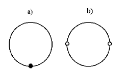
is nothing but (a part of) the renormalized one-loop self-energy correction, Fig. 1a, having the high temperature behavior (exact up to -independent constant)
| (23) | |||
| (27) |
Since in the symmetric model in the large- limit the EP can be expressed[21] in the power-series expansion in ;
| (28) |
where
| (30) | |||||
then we can easily find the solution[21] to the above posed problem; at , the “th-to-leading ” function is given solely in terms of the -loop level potential, , which is a pure constant. So if we caluculated the EP to the L-loop level, then at it already gives the function form “exact” up to “th-to-leading ” order. With the -loop potential at hand, the EP satisfying the RGE’s can be given by
| (31) | |||||
| (32) |
where the barred quantities should be evaluated at such a satisfying .
In the simple model (and also in the general symmetric model), however, because of the existence of the three-point coupling the structure of the EP in its perturbation series expansion is not the simple power-series expansion in , Eqs.(11) and (12). Thus we are forced to study more carefully the sub-structure of the perturbation series expression of the EP. We find that there is an another important effective variable
| (33) | |||
| (43) |
where
| (44) |
which is nothing but the renormalized one-loop correction to the coupling, Fig.1b, having the high temperature behavior (exact up to -independent constant)
| (45) | |||
| (49) |
represents a diagram that appears as an important sub-diagram producing large temperature-dependent corrections in the higher loop diagramms.
With the two effective variables and in hand, the EP in the massive scalar model can be expressed as a double power-series expansion in these two variables; Eq. (11) where now having the double power-series expression in and ,
| (50) |
The summation over should be taken with the constants , and .
Then the solution to the problem posed above, namely the problem how can we determine, with the limited knowledge of the -loop calculation, the function form of the EP, can be found as a simple generalization of the solution in the symmetric model; at , the “th-to-leading” function is given solely in terms of the -loop level potential, , where . Note that in the present case, being different from the large- limit of the symmetric model, can be a function of , , and of , but is importantly less than . So if we caluculated the EP to the -loop level, then at it already gives the function form “exact” up to “th-to-leading” order. With the -loop potential at hand, the EP satisfying the RGE’s can be given by
| (51) | |||||
| (52) |
where the barred quantities, which are functions of and , should be evaluated at such and satisfying
| (53) |
In the RG-improved EP, Eq. (18), the highest series of contributions take the form , namely, contributions of nor of never appear explicitly, all resummed and absorbed into the barred quantities.
It should be noted that the two independent conditions, Eqs.(19), now fix the RS, namely guarantee to carry out the RG-improvement of the EP in the sense noted above. These two conditions actually make the one-loop radiative corrections to the mass and to the coupling totally vanish. Generally speaking we can find solutions and to Eqs.(19) if the starting perturbative calculation is performed in the -renomalization, otherwise not.
III Phase structure of the simple massive scalar model at
Now we explicitly apply the RG improvement procedure explained above to the massive scalar model at , and study the phase structure. Here we only carry out the improvement of the one-loop results. Thorough analysis including those of critical exponents and the improvement of the two-loop results will be given elsewhere[25].
A -renomalization
The perturbatively calculated one-loop EP in the -renomalization is
| (56) | |||||
where
| (57) |
At the one-loop level the mass-squared and the coupling satisfy the RGE’s,
| (58) | |||
| (59) | |||
| (60) |
To perform the RG improvement explained in the last Sec. II, we must solve these RGE’s to obtain and . Responce-equations of , Eqs.(22), can be solved analytically to get
| (61) | |||||
| (62) |
The differential equations (23) describing the responces of can not be solved exactly even at the one-loop level in the general -renomalization. Thus to study the definite results of the one-loop improvement, we must perform the numerical integration of Eqs.(23). Fortunately, however, we can find an approximate solution of in the high temperature regime,
| (63) | |||||
| (64) |
The solution is exact up to order in the high temperature (HT) expansion.
Up to now and in the above eqations (24)-(27) can be arbitrary, with and being fixed at the initial values of renormalization. Our RG-improvement procedure, i.e., the resummation procedure a la RG, can then be carried out by choosing the RS-fixing parameters and so as to satisfy , Eqs.(19), namely to make the one-loop radiative corrections to the mass and also to the coupling fully vanish. First let us see the solutions to the above RS-fixing equations. In the HT regime where , we can use the HT expansion of the functions and with ,
| (66) | |||||
| (67) |
Then the RS-fixing equations give two equations being exact up to -independent constant,
| (68) | |||
| (69) |
where . Solutions to these equations (30) and (31) are
| (70) | |||||
| (71) |
determining the RS-parameters with which the EP should be evaluated.
If we can find the exact solution to the coupled equations (23) together with the exact solution , Eqs.(24) and (25), then with the use of above solutions to the RS-parameters, Eqs.(32) and (33), we can perform the full resummation of terms together with terms of . Question: How has the resummation of terms of been carried out? Answer: It is done through the -renormalization with the RS-parameters (32) and (33), guaranteeing the renomalized mass-squared to have -dependent term . As explained above, however, the solution with compact expression, Eqs.(26) and (27), is an approximate one, thus may weaken the “full resummation” of terms.
Now let us study the consequences of the RG-improvement in the -renormalization, with solutions , Eqs.(24) and (25), , Eqs. (26) and (27), and , Eqs. (32) and (33). The mass-gap equation,
| (72) |
becomes at HT (up to )
| (73) |
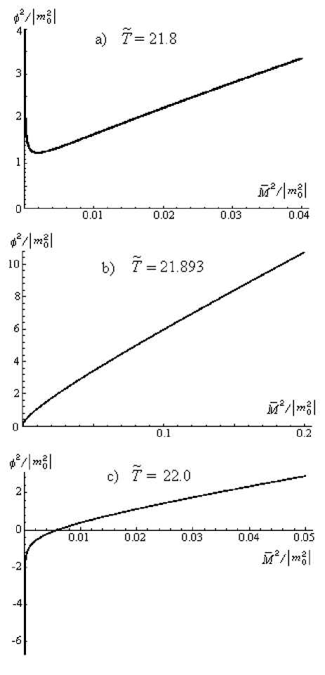
With the mass-gap equation (35) we can study as a function of , Figs.2a-2c, from which we can see the followings; i) at sufficient high temperature there is only one phase in the HT approximation and can not reach zero, Fig.2c, ii) at the critical temperature the vanish at , Fig.2b, and iii) below the critical temperature there appears a new phase in the small- region, thus the two-phase structure comes about at low temperature, Fig.2a.
By studying the structures of the RG-improved one-loop EP, ,
| (76) | |||||
| (78) | |||||
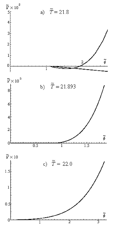
at the corresponding temperatures and phases, we can see the nature of the temperature-dependent phase-transition of the model, Figs.3a-3c; i) At low temperature below the EP has twofold structure representing the existence of two phases, Fig.3a, the ordinary mass phase and the small mass phase. The ordinary mass phase, with its counterpart in the tree-level potential, has the EP with the wine-bottle structure with the minimum at . The small mass phase is a new phase appearing as a result of resummation a la RG, without having any counterpart in the tree-level potential. This new phase is a “symmetric” phase with a linearly decreasing potential, namely with a potential unbounded from below, indicating the simple model becoming an unstable theory at low temperature. As the temperature becomes higher the minimum of the ordinary mass phase eventually diminishes, and ii) at the critical temperature the minimum of the potential at non-zero completely disappears. The EP shows a symmetric structure in with the minimum at , , , Fig.3b, and iii) at high temperature above the EP remains symmetric in whose positive curvature near becomes strong as the temperature, Fig.3c. Transition between the ordinary mass broken phase at low temperature and the symmetric phase at high temperature clearly proceeds through the second order transition.
To get more definite conclusion of the complete resummation of , we need the numerical analysis in solving exactly without HT approximation.
B -renormalization
The perturbatively calculated one-loop EP in the -renormalization is
| (81) | |||||
It is worth noting that in the -renormalization the resummation of the dominant terms can be automatically performed through renormalization, giving the renormalized mass-squared
| (82) |
the renormalized mass in the vacuum theory. appears as a mass-term in the propagator with which the perturbative calculation is performed.
At the one-loop level we can find the exact solutions of the running parameters and ,
| (83) | |||
| (84) |
As explained in the Sec.II, in the -renormalization we have only one arbitrary parameter , and we can set only one RS-fixing condition. Reminding us of the lessons from previous works[8, 13, 14, 21], we choose as a condition to fix the RS, namely choose the RS-parameter so that the one-loop radiative corrections to the mass vanish. Then the RG improvement can be performed analytically, obtaining the improved EP as
| (87) | |||||
| (88) |
All the barred quantities should be evaluated at such a satisfying the RS-fixing condition , which gives the mass gap equation
| (89) | |||||
| (90) |
It should be noted that the RS-fixing condition gives the equation at HT
| (91) |
which determines the RS-parameter as
| (92) |
In the RG-improvement with the -renormalization we can only set , thus the resummation of terms of is imcomplete. We can easily check that part of contributions coming from diagrams with three-point vertices at two-loop level can not be fully absorbed through the present improvement procedure. Such contributions can be totally absorbed if we can set the second condition as in the -renormalization case studied in the last Sec. III.A.
With the RG improved formula (40)-(47) in hand we can anyhow study the phase structure of the model as a result of the partial resummation of terms. It is surprising that all the results on the - relation and those on the corresponding EP are essentially the same as those obtained in the -renormalization case: the existence of the unstable small mass phase at low temperature, and the second order transition between the ordinary mass broken phase at low temperature and the symmetric phase at high temperature.
C renormalization
The application of the RG-inspired resummation procedure has been already carried out to the one-loop EP in the renormalization, see Nakkagawa and Yokota in [22]. Here we only would like to point out the following fact; If we start the perturbative calculation in the renormalization scheme, then the resummation of dominant corrections of should be fully accomplished through the RS-fixing condition , giving
| (93) | |||||
| (94) |
Remembering , then Eq.(49) determines the RS-parameter as
| (95) |
showing that the remaining (un-resummed) terms are actually large enough to be comparable with the contributions. This fact indicates the breakdown of the resummation method a la RG in the renormalization with the use of RS-fixing condition .
Such a trouble never happens in the -renormalization as well as in the T-renormalization studied above in Secs. III.A and III.B.
It is worth mentioning that, in the large- limit of the symmetric model, after setting there appear no remaining (un-resummed) terms, see Eqs. (11) and (12), assuring the absence of the above trouble in the renormalization.
IV Critical Exponents
Here we present the results of brief analysis of the critical exponents determined from the RG-improvement one-loop EP in the -renormalization, Sec. III.B. In this case we can calculate approximately the critical exponents through analytic manipulation.
The definition of the critical exponents are as follows:
1) On the behavior at around :
| (96) | |||||
| (97) | |||||
| (98) |
2) On the behavior at :
| (99) |
In the above, denotes the position of the true minimum, and denotes the critical temperature, which are determined as , .
Results are summarized in Table I, in which the critical exponents determined in the mean-field approximation, and in other works are also given for comparison. We can see that our results show siginificant deviations from the mean-field values, and show reasonable agreement with the experimental results.
It should be noted that our present analysis of the critical exponents is a very crude one, and further analysis including more prescise detemination through numerical evaluation as well as the analysis based on the EP determined in the -renormalization, Sec. III.C, are now in progress[25].
V Discussion and comments
In this paper we proposed a resummation method inspired by the renormalization-group improvement. By applying this resummation procedure a la RG-improvement to the one-loop effective potential in massive scalar model at , we found important observations; the temperature dependent phase transition of the model is expected to proceed through the second order transition. The critical exponents are roughly determined through analytic manipulation, showing the siginificant deviation from the mean-field values and the reasonable agreement with the experimental deta[23, 24]. This point should be made clearer with further studies on the precise determined of critical exponents of the theory which is now in progress and the results will be given elsewhere[25]. With the success in the model, it is of interest to apply the present resummation method a la RG-improvement to a more physically relevant model, such as the Abelian-Higgs model, which is now in progress.
Discussion of the results and several comments are in order.
i) Starting the perturbative calculations with the theory renormalized at an arbitrary mass-scale and at an arbitrary temperature , we can in principle fully resum terms of together with terms of . The key idea is to fix the arbitrary RS-parameters so as to make both of one-loop radiative corrections to the mass as well as to the coupling vanish. This is actually the condition which ensures the function form of the EP to be determined up to the next-to-leading order of large correction terms (see, the analysis in Sec. II, just above Eq.(18)), thus absorbing completely those terms of and of . With the use of approximate solutions to the RGE’s for the running mass-squared we can carry out the resummation program analytically, showing that the temperature-dependent transition between the symmetry-broken phase and the symmetry-restored phase proceeds through the second order phase transition. The approximation employed actually may spoil the full resummation of terms of . To make this observation concerning the order of transition in the massive scalar model more definite the RG-improvement without use of the additional approximation, together with the two-loop analysis are necessary, and are now under investigation.
ii) We can firstly renormalize the theory at the temperature of the environment . In this case -term resummation, thus the so-called hard-thermal-loop resummation[7] in this model, can be simply completed through the -renormalization itself. With the lack of freedom we can set only one RS-fixing condition to absorb the large terms of , thus only the partial resummation of these terms can be carried out. Resulting phase structure of the model is, however, essentially the same as that in the -renormalization above. In this sense our resummation method seems to give stable results so long as the terms of are systematically resummed.
iii) Our resummation method a la RG improvement does not work if we start the perturbative calculation with the theory renormalized at . In this case the condition that may ensure the resummation of large temperature-dependent corrections actually generates new large terms, thus the whole procedure of the resummation might get into trouble.
iv) As was pointed out in Sec. III, the RG-improved EP in the simple massive model has an unstable small mass phase at low temperature. This unstable small mass phase also appears in the same model at exact zero-temperature (vacuum theory), indicating its appearence being not the artifact coming from the crudeness of the resummation of temperature-dependent corrections terms. Though the origin of the appearence of this unstable phase is not fully understood, it may have a relation with the triviality of the model, which is an interesting problem for further studies.
Finally it is worth noticing that the renormalization-group analysis of the massive scalar model has been done in great details by M. van Eijck[27]. In his work the importance of the finite-temperature renormalization is clearly shown. However, the resummation of large temperature-dependent correction-terms is not the main issue of his work, thus no idea is given on the effective resummation-procedure of such terms, which our present work brings into focus.
Acknowledgments
One of us (H. N.) thanks to Prof. G. van Weert for informing the work by M. van Eijck. This work was partly supported by the Special Grant-in-Aid of the Nara University.
REFERENCES
- [1] E-mail: nakk@daibutsu.nara-u.ac.jp
- [2] E-mail: yokotah@daibutsu.nara-u.ac.jp
- [3] R. Jackiw and G. Amelino-Camelia, in Banff/CAP Workshop on Thermal Field Theory, proceedings of the 3rd Workshop on Thermal Field Theories and Their Applications, Banff, Canada, 1993, edited by F.C. Khanna, R. Kobes, G. Kunstatter and H. Umezawa (World Scientific, 1994), p.180 and references therein.
- [4] See, e.g., P. Arnold and O. Espinosa, Phys. Rev. D47, 3546 (1993); P. Fendley, Phys. Lett. B196, 175 (1987).
- [5] A. D. Linde, Rep. Prog. Phys. 42, 389 (1979); Phys. Lett. 96B, 289 (1980); D. J. Gross, R. D. Pisarski and L. G. Yaffe, Rev. Mod. Phys. 53, 43 (1981).
- [6] See, e.g., T. Muta, Foundations of Quantum Chromodynamics (World Scientific, Singapore, 1987).
- [7] E. Braaten and R. D. Pisarski, Nucl. Phys. B337, 569 (1990); ibid. B339, 310 (1990); F. Frenkel and J. C. Taylor, ibid. B334, 199 (1990).
- [8] L. Dolan and R. Jackiw, Phys. Rev. D9, 3320 (1974); M. E. Carrington, Phys. Rev. D45, 2933 (1992).
- [9] S. Leupold, hep-ph/9808424, and references therein.
- [10] J.-P.Bloizot nd E. Iancu, Nucl. Phys. B421, 565 (1994); ibid. B434, 662 (1995).
- [11] G. Amelino-Camelia, Phys. Lett. B407, 268 (1997); See also S. Chiku and T. Hatsuda, Phys. Rev. D58, 076001 (1998) (hep-ph/9803226), and references therein.
- [12] E. Braaten, Phys. Rev. Lett. 74, 2164 (1995); E. Braaten and A. Nieto, Phys. Rev. D51, 6990 (1995); ibid. D53, 3421 (1996); F. Karsch, A. Patkos and P. Petreczky, Phys. Lett, B401, 69 (1997).
- [13] G. Amelino-Camelia and S.-Y. Pi, Phys. Rev. D47, 2356 (1993).
- [14] G. Amelino-Camelia, Phys. Rev. D49, 2740 (1994); See also, C. Glenn Boyd, David E. Brahm and Stephen D.H. Hsu, ibid. D48, 4963 (1993); J.E. Bagnasco and Michael Dine, Phys. Lett. B303, 308 (1993).
- [15] P. Arnold and L.G. Yaffe, Phys. Rev. D49, 3003 (1994); K. Farakos, K. Kajantie, K. Rummukainen and M. Shaposhnikov, Nucl. Phys. B442, 317 (1995); W. Buchmüller and O. Philipsen, ibid. B443, 47 (1995).
- [16] H.-S. Roh and T. Matsui, Eur. Phys. J. A1, 205 (1998); J. Arafune, K. Ogure and J. Sato, Prog. Theor. Phys. 99, 119 (1998); T. Inagaki, K. Ogure and J. Sato, ibid. 99, 1069 (1998).
- [17] K. Ogure and J. Sato, Phys. Rev. D57, 7460 (1998).
- [18] B. Bergerhoff, hep-ph/9805493.
- [19] R. Guida and J. Zinn-Justin, Nucl. Phys. B489, 626 (1997).
- [20] M. Bando, T. Kugo, N. Maekawa and H. Nakano, Phys. Lett. B301, 83 (1993).
- [21] H. Nakkagawa and H. Yokota, Mod. Phys. Lett. A11, 2259 (1996).
- [22] Application of the RG-inspired resummation procedure in the simple massive model renormalized at zero temperature has been already done, H. Nakkagawa and H. Yokota, Prog. Theor. Phys. Suppl. 129, 209 (1997). In this case the condition that makes the resummation of dominant temperature-dependent correction-terms possible is found actually to generate new large terms, thus putting the whole pocedure into trouble, for more details see Sec. III.C below.
- [23] J. Zinn-Justin, Quantum Field Theory and Critical Phenomena (Claredon, Oxford, 1989).
- [24] H.W.J. Blöte, A. Compagner, J. H. Croockewit, Y.T.J.C. Fonk, J.R. Heringa, A. Hoogland, T.S. Smit and A.L. van Villingen, Physica A161, 1 (1989).
- [25] H. Nakkagawa and H. Yokota, papers to appear.
- [26] H. Matsumoto, Y. Nakano and H. Umezawa, Phys. Rev. D29, 1116 (1984); and Ref. [21] above.
- [27] M. van Eijck, Thermal Field Theory and the Finite-Temperature Renormalization Group, Ph.D Thesis, 1995, and references therein.
| Our result | 0.3 | 1.2 | 5.0 | 0.2 |
|---|---|---|---|---|
| mean-field | 0.5 | 1.0 | 3.0 | 0.0 |
| pertur. theory | 0.5 | 1.0 | 3.0 | 0.0 |
| (2-loop) | ||||
| auxiliary mass[17] | 0.385 | 1.37 | 4.0 | 0.12 |
| nonpertur. RG[18] | 0.35 | 1.32 | 5.0 | |
| -expansion[19] | 0.327 | 1.24 | 4.79 | 0.11 |
| lattice[24] | 0.324 | 1.24 | 4.83 | 0.113 |
| experimental[23] | 0.325 | 1.24 | 0.112 |