Abstract

We explore a model of inflation where the inflaton mass-squared is generated at a high scale by gravity-mediated soft supersymmetry breaking, and runs at lower scales to the small value required for slow-roll inflation. The running is supposed to come from the coupling of the inflaton to a non-Abelian gauge field. In contrast with earlier work, we do not constrain the magnitude of the supersymmetry breaking scale, and we find that the model might work even if squark and slepton masses come from gauge-mediated supersymmetry breaking. With the inflaton and gaugino masses in the expected range, and $\alpha=g^{2}/4\pi$ in the range $10^{-2}$ to $10^{-3}$ (all at the high scale) the model can give the observed cosmic microwave anisotropy, and a spectral index in the observed range. The latter has significant variation with scale, which can confirm or rule out the model in the forseeable future.

1 Introduction

It is well known [1, 2] that slow-roll inflation requires the flatness conditions $\epsilon\ll 1$ and $|\eta|\ll 1$ on the potential, where

$$\epsilon \equiv \frac{1}{2}M_{\rm P}^{2}\left(\frac{V^{\prime}}{V}\right)^{2}$$ (1)

$$\eta \equiv M_{\rm P}^{2}{V^{\prime\prime}\over V}\,,$$ (2)

and $M_{Pl}\equiv(8\pi G)^{-1/2}=2.4\times 10^{18}\,\mbox{GeV}$. The first condition is automatically satisfied near a maximum or minimum of the potential, where inflation is usually supposed to take place, but the second is problematic. A generic supergravity theory gives all scalar fields [3, 4], and in particular the inflaton [5, 6] a mass-squared with magnitude at least of order $V/M_{\rm P}^{2}$, which would spoil this condition. Yet supergravity is generally considered as the appropriate framework for a description of the fundamental interactions, and in particular for the description of their scalar potential.

Very few proposals have been put forward to solve this problem which would not be relying on some sort of fine tuning [2]. Our aim is to investigate in detail the proposal of Stewart [7, 8] in which loop corrections can flatten the inflaton potential without any significant fine-tuning. We follow him in assuming that the dominant corrections come from a single gauge coupling of the inflaton, and explore the region of parameter space which is allowed by the observed magnitude and spectral index of the curvature perturbation.

In the next section we give the general picture. In Section 3 we write down the Renormalization Group Equations (RGE’s) giving the scale-dependence of the inflaton mass, and hence its potential $V(\phi)$. In Section 4 we use the slow-roll approximation to derive an analytic expression for the number $N(\phi)$ of $e$-folds between a given epoch and the end of slow-roll inflation. In Section 5 we derive the predictions of the model for the spectrum of the curvature perturbation, and for its dependence on the comoving scale as specified by the spectral index $n(k)$. They depend on five parameters; the inflaton mass $m_{0}$, the gaugino mass $\tilde{m}_{0}$ and the gauge coupling $\alpha_{0}$ (all evaluated at the Planck scale, as indicated by the subscript zero, with the last two multiplied by group-theoretic factors of order 1), the magnitude $V_{0}$ of the inflaton potential, and the number $N\mathrel{\hbox to0.0pt{\lower 4.0pt\hbox{\hskip 1.0pt$\sim$}\hss}\raise 1.0pt\hbox{$<$}}55$ of $e$-folds of slow-roll inflation after a typical cosmological scale leaves the horizon. Imposing the COBE measurement of the spectrum on large scales, and the observational constraint $|1-n|<0.2$ over the whole range of cosmological scales, we find an allowed region of parameter space that includes the theoretically expected one. In Section 5 we examine various consistency conditions on the calculation. They are generally satisfied in the allowed region calculated in Section 4. Finally, we comment on the significance of the results and point out that observation will confirm or exclude the model in the forseeable future.

2 The general picture

We adopt the model of Stewart [8] (see also the review [2]). Slow-roll inflation occurs, with the following Renormalization Group improved potential for the canonically normalized inflaton field $\phi$;

$$V=V_{0}+\frac{1}{2}m^{2}(\phi)\phi^{2}+\cdots\,.$$ (3)

The constant term $V_{0}$ is supposed to dominate at all relevant field values. Non-renormalizable terms, represented by the dots, give the potential a minimum at large $\phi$, but they are supposed to be negligible during inflation. The inflaton mass-squared $m^{2}(Q)$ depends on the renormalization scale $Q$, and following [7, 8] we have taken

$$Q=\phi$$ (4)

so that loop corrections will hopefully be small.

At the Planck scale $\phi=M_{\rm P}$, $m^{2}(\phi)$ is supposed to be negative, with the generic magnitude

$$|m^{2}_{0}|=|m^{2}(M_{P})|\sim V_{0}/M_{\rm P}^{2}$$ (5)

If there were no running, this would give $|\eta|\sim 1$, preventing inflation. But at small field values, the RGE’s drive $m^{2}(\phi)$ to small values, corresponding to $|\eta(\phi)|\ll 1$, and slow-roll inflation can take place there. Within this region, there is a maximum of the potential, and we assume that the inflaton initially finds itself to the left of the maximum.

Slow-roll inflation is assumed to continue until some epoch $\phi_{\rm end}$, when $\eta(\phi)$ becomes of order $+1$. Then $\phi$ starts to oscillate around the origin, but inflation does not end because $V$ is still dominated by the constant term $V_{0}$. In order to end inflation, we need a hybrid mechanism where $V_{0}$ comes from the displacement of another field $\psi$ from its vacuum value. When the amplitude of the $\phi$ oscillation falls below some critical value $\phi_{\rm c}$, the other field $\psi$ rolls towards its vacuum value.

Inflation finally ends some number $N_{\rm fast}$ of $e$-folds after the end of slow-roll inflation, when $\phi$ and $\psi$ both settle down to their vacuum values. For us this number is a free parameter, since we are not specifying the complete potential which anyhow would probably contain free parameters.

Let us be more specific about the expected magnitude of $m^{2}$ at the Planck scale, Eq. (5). We are assuming that the potential comes from the $F$ term of a supergravity theory, containing chiral superfields whose scalar components are complex fields $\phi_{n}$. The real inflaton field $\phi$ is supposed to be a quasi-flat direction in this multi-field space. Making the usual assumption that any fermion condensates can be represented as a non-perturbative contribution to the superpotential, the $F$ term has the familiar form

$$V = M_{\rm inf}^{4}-3e^{K/M_{\rm P}^{2}}M_{\rm P}^{-2}|W|^{2}$$ (6)

$$M_{\rm inf}^{4} \equiv e^{K/M_{\rm P}^{2}}\left(W_{n}+M_{\rm P}^{-2}WK_{n}\right)K^{nm^{\star}}\left(W_{m}+M_{\rm P}^{-2}WK_{m}\right)^{\star}\,.$$ (7)

Here $W$ is the superpotential, a holomorphic function of the $\phi_{n}$, and $K$ is the Kähler potential, a real function of the $\phi_{n}$ and their complex conjugates. A subscript $n$ denotes $\partial/\partial\phi_{n}$ while $n^{\star}$ denotes $\partial/\partial\phi_{n}^{\star}$, and $K^{nm^{\star}}$ is the matrix inverse of $K_{nm^{\star}}$.

The quantity $M_{\rm inf}$ may be taken to define the scale of supersymmetry breaking during inflation. (The similarly-defined quantity in the vacuum is generally denoted by $M_{\rm S}$.) An essential assumption is that the inflaton mass is negligible in the limit of global supersymmetry, and comes only from supergravity corrections. The mass-squared of the inflaton (and of any other scalar field receiving its mass only from supergravity) is then given by

$$M_{\rm P}^{2}m^{2}=V\pm cM_{\rm inf}^{4}\,..$$ (8)

The first term comes [5, 6] from the factor $e^{K/M_{\rm P}^{2}}$. The factor $c$ in the second term receives contributions from non-renormalizable terms in $K$ [2]. In units of $M_{\rm P}$, the coefficients of these terms are supposed to be roughly of order 1 at the Planck scale. This gives $c\sim 1$, within some uncertainty factor $10^{\Delta}$ that is a matter of taste.

We now make two crucial assumptions. One is that, in contrast with the case for the vacuum, there is no strong cancellation between the two terms of Eq. (6), so that $V\sim M_{\rm inf}^{4}$. The validity of this assumption could be checked in a particular model. Second, there is no strong cancellation between the two terms of Eq. (8). This second assumption is a statement about the non-renormalizable terms of $K$, whose status is hard to judge. A strong cancellation might happen by accident, or because we are dealing with a model in which $K$ and $W$ have special forms that ensure the cancellation [11, 2]. For the purpose of this paper, we are taking the view that a strong cancellation is unlikely.

With these assumptions, the expected value of the inflaton mass-squared at the Planck scale is

$$1\mathrel{\hbox to0.0pt{\lower 4.0pt\hbox{\hskip 1.0pt$\sim$}\hss}\raise 1.0pt\hbox{$<$}}M_{\rm P}^{2}|m^{2}(M_{\rm P})|/V_{0}\mathrel{\hbox to0.0pt{\lower 4.0pt\hbox{\hskip 1.0pt$\sim$}\hss}\raise 1.0pt\hbox{$<$}}10^{\Delta}\,,$$ (9)

with the value $\sim 1$ regarded as the most likely, and values $\ll 1$ regarded as unlikely.

It is instructive to compare this analysis with the usual one, which applies in the vacuum. Here, the mass-squared of a scalar field, if it comes only from supergravity, is given by the analogue of Eq. (8), $M_{\rm P}^{2}m^{2}=\pm cM_{\rm S}^{4}$, the supersymmetry breaking scale $M_{\rm S}$ being related to the potential by Eq. (6) with $M_{\rm inf}$ replaced by $M_{\rm S}$. The contribution to $M_{\rm P}^{2}m^{2}$ from $V$ is now absent, because $V$ vanishes in the vacuum. As a result it is equally reasonable to expect $m^{2}$ to be a factor $10^{\Delta}$ above or below the estimate $M_{\rm P}^{2}m^{2}\sim M_{\rm S}^{4}$. There is no prejudice against values below, as is the case during inflation.

In summary, we have seen that achieving the slow-roll requirement $M_{\rm P}^{2}|m^{2}|\ll V_{0}$ on the inflaton mass is not just a matter of tuning something a bit below its expected value. Rather, one has to invoke a strong cancellation between different contributions. The idea of the present model is to avoid that, by running the inflaton mass.

In the limit where the inflaton mass has negligible scale dependence, we arrive at the tree-level model of Randall, Soljacic and Guth [13], which invoked an accidental cancellation to keep the inflaton mass sufficiently small. Apart from avoiding the cancellation, the strong running of the inflaton mass invoked in the present model has another advantage [8], which is that slow-roll inflation can (and is supposed to) end before $\phi$ reaches the critical value $\phi_{\rm c}$. This makes the predictions practically independent of $\phi_{\rm c}$. It also reduces, or maybe eliminates, the dangerous spike in the spectrum of the curvature perturbation, that is generated in the tree-level model after slow-roll inflation ends.

The tree-level model [13], and Stewart’s paper [8], actually made two assumptions, beyond the ones mentioned already. First, that the scales of supersymmetry breaking during inflation and in the vacuum are similar, $M_{\rm S}\sim M_{\rm inf}\simeq V^{1/4}$. Second, that the squarks and sleptons of the supersymmetric Standard Model also get their masses only from supergravity (gravity-mediated supersymmetry breaking). With these assumptions one will have roughly $V_{0}^{1/4}\sim\sqrt{m_{\rm s}M_{\rm P}}\sim 10^{10}\,\mbox{GeV}$ where $m_{\rm s}$ roughly of order $100\,\mbox{GeV}$ is the expected mass of squarks and sleptons. We shall not make these assumptions, and leave $V_{0}$ as an essentially free parameter. If we retain the first assumption, but assume [2] that the squark and slepton masses of the supersymmetric Standard Model are gauge-mediated, we will have $10^{5}\,\mbox{GeV}\mathrel{\hbox to0.0pt{\lower 4.0pt\hbox{\hskip 1.0pt$\sim$}\hss}\raise 1.0pt\hbox{$<$}}V_{0}^{1/4}\mathrel{\hbox to0.0pt{\lower 4.0pt\hbox{\hskip 1.0pt$\sim$}\hss}\raise 1.0pt\hbox{$<$}}10^{10}\,\mbox{GeV}$. We stress that the latter case can only be realised when the inflaton sector is different, and decoupled from, the visible sector, due to our assumption that the inflaton mass is generated by gravity-mediated soft supersymmetry breaking.

3 The Renormalization Group Equations

We assume that in the inflaton sector, the RGE’s are those of softly broken global supersymmetry. To obtain the functional form of $m^{2}(Q)$ we follow Stewart [8] in assuming that the inflaton has a gauge coupling, which dominates the RGE’s. (This is a hybrid inflation model, so the inflaton certainly has Yukawa couplings but they are assumed to have a negligible effect.)

The RGE’s will involve the gaugino mass $\tilde{m}(Q)$. In contrast with the case of scalar masses, gaugino masses might a priori be very small, because they depend on the gauge kinetic function $f$. Allowing for this possibility, the expected value of the gaugino mass at the Planck scale is therefore $0\mathrel{\hbox to0.0pt{\lower 4.0pt\hbox{\hskip 1.0pt$\sim$}\hss}\raise 1.0pt\hbox{$<$}}(M_{\rm P}^{2}\tilde{m}^{2}(M_{\rm P})/V_{0})\mathrel{\hbox to0.0pt{\lower 4.0pt\hbox{\hskip 1.0pt$\sim$}\hss}\raise 1.0pt\hbox{$<$}}1$, or allowing some uncertainty

$$0\mathrel{\hbox to0.0pt{\lower 4.0pt\hbox{\hskip 1.0pt$\sim$}\hss}\raise 1.0pt\hbox{$<$}}\frac{M_{\rm P}^{2}\tilde{m}^{2}(M_{\rm P})}{V_{0}}\mathrel{\hbox to0.0pt{\lower 4.0pt\hbox{\hskip 1.0pt$\sim$}\hss}\raise 1.0pt\hbox{$<$}}10^{\Delta}\,.$$ (10)

We also need the gauge coupling at the Planck scale, and we make the usual assumption that it is in the perturbative regime $\alpha(M_{\rm P})\mathrel{\hbox to0.0pt{\lower 4.0pt\hbox{\hskip 1.0pt$\sim$}\hss}\raise 1.0pt\hbox{$<$}}0.1$. On the other hand one does not expect it to be many orders of magnitude smaller, under the usual supposition that gauge couplings at the high scale come more or less directly from something like string theory. For definiteness, let us say that we expect

$$10^{-3}\mathrel{\hbox to0.0pt{\lower 4.0pt\hbox{\hskip 1.0pt$\sim$}\hss}\raise 1.0pt\hbox{$<$}}\alpha(M_{\rm P})\mathrel{\hbox to0.0pt{\lower 4.0pt\hbox{\hskip 1.0pt$\sim$}\hss}\raise 1.0pt\hbox{$<$}}10^{-1}\,.$$ (11)

From now on, we set $M_{\rm P}=1$ except where stated. We work at one loop order, and consider scales well above the relevant masses,

$$\tilde{m}(Q),\ m(Q)\ll Q\,.$$ (12)

The RGE’s have the same form as the well-known ones that describe the running of the squark masses with only QCD included,

$${d\alpha\over dt} = {b\over 2\pi}\alpha^{2}$$ (13)

$${d\over dt}\left({\tilde{m}\over\alpha}\right) = 0$$ (14)

$${dm^{2}_{\phi}\over dt} = -{2c\over\pi}\alpha\tilde{m}^{2}$$ (15)

Here $\alpha$ is related to the gauge coupling by $\alpha=g^{2}/4\pi$, and $t\equiv\ln Q<0$. The numbers $b$ and $c$ depend on the group; $c$ is the Casimir quadratic invariant of the inflaton representation under the gauge group, for instance $c=(N^{2}-1)/2N$ for any fundamental representation of $SU(N)$, and $b=-3N+N_{\rm f}$ for a supersymmetric $SU(N)$ with $N_{\rm f}$ pairs of fermions in the fundamental/antifundamental representation. It is not clear whether one can construct a model in which the gauge group is actually the $SU(3)$ of QCD. All we assume for the moment is that $c$ and $-b$ are positive.

Using a subscript 0 to denote the Planck scale $t=\ln M_{\rm P}=0$, the solutions of equations (13)-(15) are

$$\alpha(t) = {\alpha_{0}\over 1-{b\alpha_{0}\over 2\pi}t}$$ (16)

$$\tilde{m}(t) = {\tilde{m}_{0}\over 1-{b\alpha_{0}\over 2\pi}t}$$ (17)

$$m^{2}(t) = m^{2}_{0}+{2c\over b}\tilde{m}^{2}_{0}{\left[1-{1\over\left[1-{b\alpha_{0}\over 2\pi}t\right]^{2}}\right]}$$ (18)

We are taking $b<0$ and $c>0$, which means that $\alpha$, $\tilde{m}$ and $m$ all increase as the scale decreases, and that $m^{2}$ can cross from negative to positive values.

3.1 The field dynamics

We are making the identification $\phi=Q$, corresponding to $\ln\phi=t$. It is useful to define the following quantities

$$\mu^{2} \equiv -m^{2}/V_{0}$$ (19)

$$A = {2c\over|b|}{\tilde{m}^{2}\over V_{0}}$$ (20)

$$\tilde{\alpha} = {|b|\alpha\over 2\pi}\,.$$ (21)

(Remember that we are setting $M_{\rm P}=1$.) For $SU(N)$ (and $b<0$ as we are assuming) one has

$$|b| = 3N-N_{\rm f}$$ (22)

$$\frac{2c}{|b|} = \frac{1-N^{-2}}{3-N_{\rm f}/N}\,.$$ (23)

At least in this case, one can expect $A\simeq\tilde{m}^{2}/V_{0}$ and $\tilde{\alpha}\simeq\alpha$. With this assumption, the expected values at $M_{\rm P}$ corresponding to Eqs. (9), (10) and (11) are

$$1 \mathrel{\hbox to0.0pt{\lower 4.0pt\hbox{\hskip 1.0pt$\sim$}\hss}\raise 1.0pt\hbox{$<$}} \mu_{0}^{2}\mathrel{\hbox to0.0pt{\lower 4.0pt\hbox{\hskip 1.0pt$\sim$}\hss}\raise 1.0pt\hbox{$<$}}10^{\Delta}$$ (24)

$$0 \mathrel{\hbox to0.0pt{\lower 4.0pt\hbox{\hskip 1.0pt$\sim$}\hss}\raise 1.0pt\hbox{$<$}} A_{0}\mathrel{\hbox to0.0pt{\lower 4.0pt\hbox{\hskip 1.0pt$\sim$}\hss}\raise 1.0pt\hbox{$<$}}10^{\Delta}$$ (25)

$$10^{-3} \mathrel{\hbox to0.0pt{\lower 4.0pt\hbox{\hskip 1.0pt$\sim$}\hss}\raise 1.0pt\hbox{$<$}} \tilde{\alpha}_{0}\mathrel{\hbox to0.0pt{\lower 4.0pt\hbox{\hskip 1.0pt$\sim$}\hss}\raise 1.0pt\hbox{$<$}}10^{-1}\,..$$ (26)

Choosing $\mu^{2}_{0}=A_{0}=1$ and $\tilde{\alpha}_{0}=0.01$, we plot the potential in Figure 1.

Defining

$$\gamma\equiv\mu^{2}+{1\over 2}{d\mu^{2}\over dt}\,,$$ (27)

the derivatives of the potential Eq. (3) with respect to $\phi$ are

$$V^{\prime} = -V_{0}\phi\left[\mu^{2}+{1\over 2}{d\mu^{2}\over dt}\right]=V_{0}\phi\ \gamma$$ (28)

$$V^{\prime\prime} = -V_{0}\left[\mu^{2}+{3\over 2}{d\mu^{2}\over dt}+{1\over 2}{d^{2}\mu^{2}\over dt^{2}}\right]\,.$$ (29)

Each derivative of $\mu^{2}$ is suppressed by a factor $\tilde{\alpha}_{0}$ with respect to $\mu^{2}$. As a result [7] the flatness conditions Eqs. (1) and (2) are satisfied in a region around $V^{\prime}=0$, allowing inflation to take place there.

Figure 1: One loop potential $V/V_{0}-1$ for $\mu^{2}_{0}=A_{0}=1$ and $\tilde{\alpha}_{0}=0.01$, as a function of the scale $Q=\phi$.

Figure 2: The functions $\mu^{2}$, $\gamma$ and $\eta$ for $\mu^{2}_{0}=A_{0}=1$ and $\tilde{\alpha}_{0}=0.01$, as a function of the scale $Q=\phi$.

The flatness parameters are

$$\eta \simeq \gamma+{d\gamma\over dt}=-\left[\mu^{2}+{3\over 2}{d\mu^{2}\over dt}+{1\over 2}{d^{2}\mu^{2}\over dt^{2}}\right]$$ (30)

$$\epsilon = \frac{1}{2}\gamma^{2}\phi^{2}\ll|\eta|\,.$$ (31)

The last two terms of Eq. (30) are generically small with respect to $\mu^{2}$, but not in the region of interest $\mu^{2}\simeq 0$.

In Figure 2 we plot the quantities $\mu^{2}$, $\gamma$ and $\eta$ for a representative case.

The classical equation of motion for the inflaton field is

$$\ddot{\phi}+3H\dot{\phi}+V^{\prime}=0\,,$$ (32)

where $H^{2}=(V+\dot{\phi}^{2}/2)/3$ is the Hubble parameter. For a wide range of initial conditions, the flatness conditions lead to the slow-roll approximation

$$3H\dot{\phi}=-V^{\prime}\,.$$ (33)

We assume that slow-roll inflation ends at $\phi_{\rm end}$, defined by

$$\eta(\phi_{\rm end})=1.$$ (34)

To impose observational constraints on the model, we shall need the number of $e$-folds $N(\phi)$ of slow-roll inflation, taking place after a given epoch $\phi$. Using the slow-roll approximation and $t=\ln\phi$, it is given by

$$N=\int_{t_{\rm end}}^{t}{dt\over\gamma}\ \ .$$ (35)

To evaluate the integral, we define

$$y\equiv(1+\tilde{\alpha}_{0}t)^{-1}=(1+\tilde{\alpha}_{0}\ln\phi)^{-1}\,.$$ (36)

As $\phi$ decreases from $\phi=M_{\rm P}=1$, $y$ increases from $y_{0}=1$. We define the epoch $y_{\star}$ by $\gamma=0(=V^{\prime})$, and the epoch $y_{\star\star}$ by $\mu^{2}=0(=m^{2})$. The latter is given by

$$y_{\star\star}=\sqrt{1+{\mu_{0}^{2}\over A_{0}}}\,.$$ (37)

In terms of these quantities

$$\tilde{\alpha}(y) = \tilde{\alpha}_{0}y$$ (38)

$$A(y) = A_{0}y^{2}$$ (39)

$$\mu^{2}(y) = A_{0}\left[y_{\star\star}^{2}-y^{2}\right]$$ (40)

$$\gamma(y) = -A_{0}\left[y_{\star\star}^{2}-y^{2}+\tilde{\alpha}_{0}y^{3}\right]$$ (41)

$$\eta(y) = -A_{0}\left[y_{\star\star}^{2}-y^{2}+3\tilde{\alpha}_{0}y^{3}-3\tilde{\alpha}_{0}^{2}y^{4}\right].$$ (42)

Notice that $A$ and $-\mu^{2}$ differ only by a constant.

To first order in $\tilde{\alpha}_{0}$, the equation $\gamma=0$ has the roots $y_{\star}$ and $y_{\pm}$ given by

$$y_{\star} \simeq y_{\star\star}(1+{1\over 2}\tilde{\alpha}_{0}y_{\star\star})\,,$$ (43)

$$y_{\pm} = {1-\tilde{\alpha}_{0}y_{\star}\over 2\tilde{\alpha}_{0}}\pm\sqrt{{(1+\tilde{\alpha}_{0}y_{\star})^{2}\over 4\tilde{\alpha}_{0}^{2}}-y_{\star}^{2}}\ \simeq\left\{\begin{array}[]{c}1/\tilde{\alpha}_{0}\\ -y_{\star}\end{array}\right.$$ (46)

We are assuming that the potential has a maximum, corresponding to real $y_{\star}$. This implies that $y_{+}$ is also real (because there is always a real root $y_{-}<0$). The root $y_{+}$ represents a minimum of the potential, but since it lies in the regime of strong coupling it can hardly be trusted. Whether or not it is a real effect, we need to assume that slow-roll inflation ends before it is reached, corresponding to $y_{+}>y_{\rm end}$. According to Eq. (43), the maximum of the potential is close to the point where $m^{2}$ passes through zero.

Using these expressions,

$$N(y) = -{1\over\tilde{\alpha}_{0}}\int_{y_{\rm end}}^{y}{dy\over y^{2}\gamma(y)}$$

$$= {1\over A_{0}\tilde{\alpha}_{0}}\left[{1\over y_{\star\star}}\left({1\over y}-{1\over y_{\rm end}}\right)+{1\over\tilde{\alpha}_{0}y^{2}_{+}(y_{+}-y_{-})(y_{+}-y_{\star})}\ln\left({y_{+}-y\over y_{+}-y_{\rm end}}\right)\right.+$$

$$+ {1\over\tilde{\alpha}_{0}y^{2}_{-}(y_{+}-y_{-})(y_{\star}-y_{-})}\ln\left({y-y_{-}\over y_{\rm end}-y_{-}}\right)-$$

$$- \left.{1\over\tilde{\alpha}_{0}y^{2}_{\star}(y_{+}-y_{\star})(y_{\star}-y_{-})}\ln\left({y-y_{\star}\over y_{\rm end}-y_{\star}}\right)\right]$$ (48)

Apart for the mild dependence hidden in $y_{\rm end}$, the number of e-folds given by eq. (48) is inversely proportional to $A_{0}$; the dependence on $\tilde{\alpha}_{0}$ is more complex, but anyway a small coupling increases $N$.

We have solved the second order equation (32) numerically in the region of interest and compared the number of e-folds with the slow-roll result, Eq. (48). The latter is a good approximation over all the range considered, giving at most an error $\Delta N=2$ to 3, and we use it in what follows. (In [7, 8] the slow-roll approximation was replaced by a different approximation.)

4 The observational constraints

The vacuum fluctuation of the inflaton fields generates a primordial adiabatic density perturbation, whose spectrum ${\cal P}_{\cal R}$ is given by

$$\frac{4}{25}{\cal P}_{\cal R}\equiv\delta_{H}^{2}(k)=\frac{1}{75\pi^{2}}\frac{V^{3}}{V^{\prime 2}}=\frac{1}{150\pi^{2}}\frac{V}{\epsilon}.$$ (49)

The right hand side is evaluated at the epoch of horizon exit, $k=aH$.

The spectrum is constrained by observations of galaxies and of the cosmic microwave background (cmb) anisotropy [1, 2]. These measurements explore scales (the ‘cosmological scales’) ranging from the size of the observable Universe down to around four orders of magnitude smaller. Near the top end of the range the COBE measurement of the cmb gives an accurate value [14] for the spectrum, $\delta_{H}=1.91\times 10^{-5}$ (the uncertainty is of order $10\%$, ignoring gravitational waves). The dependence of the spectrum on the comoving wavenumber $k$ is defined through the spectral index $n$;

$$n(k)-1\equiv d{\cal P}_{\cal R}/d\ln k\,.$$ (50)

Assuming that the $n$ is slowly varying over the cosmological range, observation requires something like $|n-1|<0.2$.

The perturbation on a comoving scale with wavenumber $k/a(t)$ is generated at the epoch of horizon exit $k=aH$, which is proportional to $a\propto e^{Ht}$ in the slow-roll approximation. Hence the four-decade span of cosmological scales corresponds to $\Delta N\simeq\ln 10^{4}\simeq 9$. If there is no further inflation, the value of $N$ at the top end of the range is [1, 2]

$$N_{\rm COBE}=48-\ln(10^{10}\,\mbox{GeV}/V_{0}^{1/4})-\frac{1}{3}\ln(V_{0}^{1/4}/\rho_{\rm reh}^{1/4})\,,$$ (51)

where $\rho_{\rm reh}$ is the energy density at the ‘reheat’ temperature marking the beginning of radiation domination. As the notation indicates, we take the top end of the range to be the scale probed by COBE, though the latter is actually somewhat lower.

In the present model some number $N_{\rm fast}$ of $e$-folds of inflation take place after slow-roll ends [8]. Also, there could one or more bouts of thermal inflation before final reheating [15], each bout lasting for of order 10 $e$-folds. These reduce $N_{\rm cosm}$ by an amount $N_{\rm fast}+N_{\rm thermal}$, so $N_{\rm COBE}$ is a free parameter of the model subject to the constraint

$$10\mathrel{\hbox to0.0pt{\lower 4.0pt\hbox{\hskip 1.0pt$\sim$}\hss}\raise 1.0pt\hbox{$<$}}N_{\rm COBE}<48-\ln(10^{10}\,\mbox{GeV}/V_{0}^{1/4})-\frac{1}{3}\ln(V_{0}^{1/4}/\rho_{\rm reh}^{1/4})\,.$$ (52)

(The lower limit comes from the requirement that the perturbation is generated on all cosmological scales.)

The COBE normalization corresponds to

$${V^{3/2}\over V^{\prime}}\simeq 6\times 10^{-4}\,,$$ (53)

and the spectral index is given by

$$n-1=2\eta\,.$$ (54)

With our potential, the COBE normalization gives

$${V_{0}^{1/2}\over\gamma(y)}\exp\left[{1\over\tilde{\alpha}_{0}}\left(1-{1\over y}\right)\right]=6\times 10^{-4}\,,$$ (55)

and

$$n-1=-2A_{0}\left(y^{2}_{\star\star}-y^{2}+3\tilde{\alpha}_{0}y^{3}-3\tilde{\alpha}_{0}^{2}y^{4}\right)\,.$$ (56)

In these expressions we regard $y$ as a function of $N$ (the inverse of Eq. (48)), and it should be evaluated at the epoch of horizon exit for the relevant scale, $k=aH$. In Eq. (55), the value of $y$ is fixed, corresponding to the COBE scale which is in the upper part of the cosmological range.

It is not possible to explore the parameter space analytically without simplifying assumptions; we will therefore solve the problem numerically and explore the region in the theoretically allowed parameter space where the spectral index satisfies the experimental bound.

Taking $N_{\rm COBE}=45$, we show in Figure 3 some lines of constant $V_{0}$, in the $\mu_{0}^{2}$-$A_{0}$ plane for some choices of $\alpha_{0}$. We also show some lines of constant $n$, evaluated also at the COBE scale.

Keeping the choice $N_{\rm COBE}=45$, we show in Figure 4 the dependence of the spectral index on the comoving scale, for fixed values of $A_{0}$ and $\mu_{0}$ and the same values of $\alpha_{0}$. The variable used to specify the comoving wavenumber $k$ is $N(\phi)=\ln(k_{\rm end}/k)$, where $\phi$ is the epoch of horizon exit $k=aH$ and $k_{\rm end}$ corresponds to the end of slow-roll inflation. Cosmological scales correspond to $35\mathrel{\hbox to0.0pt{\lower 4.0pt\hbox{\hskip 1.0pt$\sim$}\hss}\raise 1.0pt\hbox{$<$}}N(\phi)\mathrel{\hbox to0.0pt{\lower 4.0pt\hbox{\hskip 1.0pt$\sim$}\hss}\raise 1.0pt\hbox{$<$}}45$.

Quite generally, there is significant variation over the range of cosmological scales. For instance, one can show that at $n=1$,

$$\frac{dn}{dN}\simeq-8A_{0}^{2}\tilde{\alpha}_{0}^{2}\left(1+\frac{\mu_{0}^{2}}{A_{0}}\right)^{3}\,.$$ (57)

Over the cosmological range $\delta N\simeq 10$ one typically has at $\delta n\sim 0.1$, which should be detectable with the advent of the MAP satellite and new galaxy surveys.

One can use Figure 4 to determine the effect of changing $N_{\rm COBE}$, on the curves of constant $n$ in Figure 3. For example, each of them has $n(45)\simeq 1.0$, and $n(30)\simeq 1.2$; therefore changing to $N_{\rm COBE}\simeq 30$ corresponds to shifting the curves $n=1.0$ in Figure 3 to the location of the curves $n=1.2$, and shifting the curves $n=0.8$ to the location $n=1.0$.

Figure 3: Contour levels of the spectral index and of $V_{0}$ in the $\mu^{2}_{0}-A$ plane for the different values of the coupling ($\tilde{\alpha}_{0}=0.1,0.05,0.01,0.001$). Notice that for $\tilde{\alpha}_{0}=0.1$ (upper left plot) a small strip of the parameter space is excluded by the consistency constraints (see Fig. 5): the unlabelled vertical line on the left indicates such constraint and is not a contour level. In the other cases the whole parameter region displayed here is contained in the allowed region of Fig. 5.

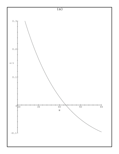
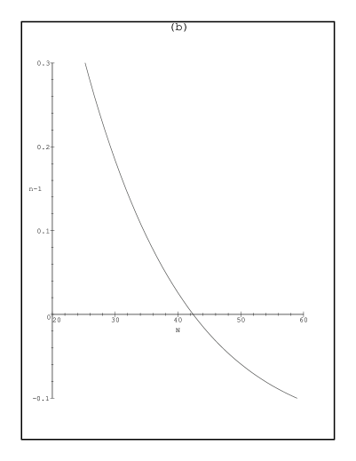
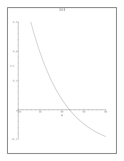
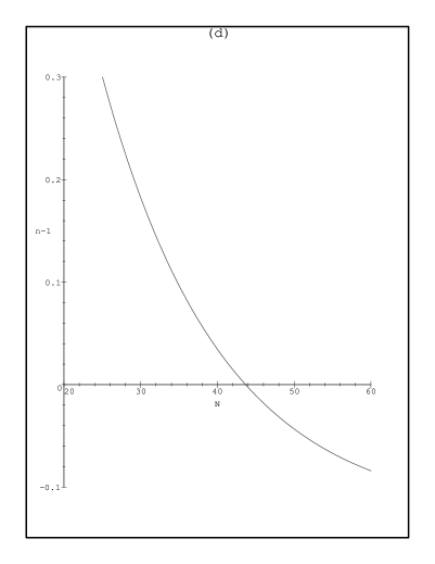
Figure 4: The spectral index as a function of comoving wavenumber. The variable used is $N(\phi)\equiv\ln(k_{\rm end}/k)$, as described at the end of Section 4. Cosmological scales are assumed to correspond to $40\mathrel{\hbox to0.0pt{\lower 4.0pt\hbox{\hskip 1.0pt$\sim$}\hss}\raise 1.0pt\hbox{$<$}}N(\phi)\mathrel{\hbox to0.0pt{\lower 4.0pt\hbox{\hskip 1.0pt$\sim$}\hss}\raise 1.0pt\hbox{$<$}}50$. Each plot corresponds to a representative point on the corresponding plot of Figure 3; (a) $\tilde{\alpha}_{0}=0.1,A_{0}=0.2,\mu^{2}_{0}=0.1$; (b) $\tilde{\alpha}_{0}=0.05,A_{0}=0.4,\mu^{2}_{0}=0.2$; (c) for $\tilde{\alpha}_{0}=0.01,A_{0}=1.7,\mu^{2}_{0}=1$; (d) for $\tilde{\alpha}_{0}=0.001,A_{0}=30,\mu^{2}_{0}=1.5$.

5 Consistency constraints

In addition to the observational constraints, we need to impose consistency conditions on the calculation.

Two of these are the constraints already imposed, namely the condition $y_{+}>y_{\rm end}$ which corresponds to the statement that slow-roll inflation ends before the minimum represented by $y_{+}$ is reached, and the condition that $y_{\star}$ is real representing the condition that the potential possesses a maximum.

Since $\eta(y)$ is an increasing function of $y$, the first of these constraints is equivalent to

$$1=\eta(y_{\rm end})\leq\eta(y_{+})=3A_{0}\tilde{\alpha}_{0}y_{+}^{3}\left[\tilde{\alpha}_{0}y_{+}-{2\over 3}\right].$$ (58)

Using expression (46) for small $\tilde{\alpha}_{0}y_{\star}$ and approximating $y^{2}_{\star}$ with $y^{2}_{\star\star}$ keeping only the leading order in the gauge coupling, gives the lower bound for $A_{0}$:

$$A_{0}\geq{\tilde{\alpha}_{0}^{2}(1+{21\over 4}\mu_{0}^{2})\over 1-{21\over 4}\tilde{\alpha}_{0}^{2}}>\tilde{\alpha}_{0}^{2}.$$ (59)

The second requirement is equivalent to the statement that Eq. (41) has three real roots, which is

$$\mu_{0}^{2}\leq\left({4\over 27\tilde{\alpha}^{2}_{0}}-1\right)A_{0}.$$ (60)

These two requirements are satisfied everywhere in the regions of parameter space shown in Figure 3, except for Figure 3a where the first requirement corresponds to the nearly vertical line on the left hand side. They are plotted in Figure 5.

There are additional requirements, which also turn out not to be significant in practice. Let us mention them briefly.

Since we are using the one-loop approximation, we should require $\tilde{\alpha}(Q)\ll 1$ for all $Q$ in the slow-roll regime $Q(=\phi)>\phi_{\rm end}$. But by virtue of the first line of Eq. (46), this is ensured by the condition $y_{\rm end}<y_{+}$ that we imposed earlier.

Figure 5: The region in the $\mu^{2}_{0}-A_{0}$ plane allowed by the consistency checks for the different values of the coupling ($\tilde{\alpha}_{0}=0.1,0.05,0.01,0.001$) is below the curves down to the x-axis. They represent Eqs. (59) (dotted line), (60) (dashed line) and (61) (full line).

Another condition is the requirement $|\eta(\phi)|<1$, which must hold throughout inflation. Recall that $\eta$ is a decreasing function of $\phi$, starting at $+1$ when $\phi=\phi_{\rm end}$, and ending at $\phi=M_{\rm P}$ with some value $\eta(M_{\rm P})\simeq\mu_{0}^{2}$. We are taking the latter value to be roughly of order 1, but if it bigger then the requirement that $|\eta|<1$ throughout slow-roll inflation could in principle be violated. To be generous, let us impose this requirement for all $\phi<\phi_{\star\star}$, which includes all $\phi<\phi_{\star}$ (the position of the maximum) and therefore all values of $\phi$ that we could possibly be interested in. This gives the relation

$$\mu_{0}^{2}\leq\left({A_{0}\over 9\tilde{\alpha}^{2}_{0}}\right)^{1/3}-A_{0}\,,$$ (61)

which is also shown in Figure 5.

A more involved requirement is $\tilde{m},m\ll g\phi$ for all values of $\phi$ during slow-roll inflation, corresponding to Eq. (12). The most stringent bound is given by the inequalities evaluated at $y_{\rm end}$:

$$\tilde{m}^{2}_{0}\ y^{2}_{\rm end}={|b|\over 2c}V_{0}A_{0}\ y^{2}_{\rm end}\ll\alpha(y_{\rm end})\phi^{2}_{\rm end}={2\pi\over|b|}\tilde{\alpha}_{0}y_{\rm end}\exp\left[-2{y_{\rm end}-1\over\tilde{\alpha}_{0}y_{\rm end}}\right]$$ (62)

and

$$V_{0}|\mu^{2}(y_{\rm end})|=V_{0}A_{0}(y_{\rm end}^{2}-y^{2}_{\star\star})\ll\alpha(y_{\rm end})\phi^{2}_{\rm end}={2\pi\over|b|}\tilde{\alpha}_{0}y_{\rm end}\exp\left[-2{y_{\rm end}-1\over\tilde{\alpha}_{0}y_{\rm end}}\right].$$ (63)

Assuming the COBE normalization, and $|b|$ and $c$ very roughly of order 1, these bounds are weaker than the condition in eq. (61) and therefore they are always satisfied in the region shown in Fig. 3a-d in the plane $\mu^{2}_{0}$ vs $A_{0}$ for different values of $\tilde{\alpha}_{0}$. Notice that the larger is $\tilde{\alpha}_{0}$, the smaller the allowed region since most of the bounds scale as negative powers of the gauge coupling.

Finally, we consider the requirement that the quantum fluctuation of the inflaton field does not come to dominate the classical slow-roll behaviour before slow-roll ends. This is equivalent to a constraint on the magnitude of the curvature perturbation calculated from slow-roll inflation, ${\cal P}_{\cal R}(k)\mathrel{\hbox to0.0pt{\lower 4.0pt\hbox{\hskip 1.0pt$\sim$}\hss}\raise 1.0pt\hbox{$<$}}1$. We find that for typical values of the parameters, this condition is satisfied until just before $\phi$ reaches the value $\phi_{\rm end}$, that corresponds to $\eta=1$. Probably, this means that the quantum fluctuation never spoils slow-roll inflation. On the other hand, such a big fluctuation might produce dangerous black holes, so one probably ought to demand a tighter upper limit than just ${\cal P}_{\cal R}(k)\mathrel{\hbox to0.0pt{\lower 4.0pt\hbox{\hskip 1.0pt$\sim$}\hss}\raise 1.0pt\hbox{$<$}}1$. An investigation of this, and other aspects of the astrophysics, will be reported in a future publication.

6 Discussion

We have explored the parameter space of a model of inflation with a running inflaton mass, and the essential result is displayed in Figure 3. Up to group-theoretic factors that are expected to be of order 1, $\mu_{0}^{2}$ is the expected magnitude of the inflaton mass-squared at the Planck scale, and $A_{0}$ is the expected value of the gaugino mass-squared, both in units of $V_{0}/M_{\rm P}^{2}$. With the assumptions mentioned in Section 2, the expected magnitudes are $\mu_{0}^{2}\sim 1$ and $A_{0}\sim 0$ to $1$. Taking for definiteness an uncertainty $10^{\Delta}=100$, the ranges $1\mathrel{\hbox to0.0pt{\lower 4.0pt\hbox{\hskip 1.0pt$\sim$}\hss}\raise 1.0pt\hbox{$<$}}\mu_{0}^{2}\mathrel{\hbox to0.0pt{\lower 4.0pt\hbox{\hskip 1.0pt$\sim$}\hss}\raise 1.0pt\hbox{$<$}}100$ and $0\mathrel{\hbox to0.0pt{\lower 4.0pt\hbox{\hskip 1.0pt$\sim$}\hss}\raise 1.0pt\hbox{$<$}}A_{0}\mathrel{\hbox to0.0pt{\lower 4.0pt\hbox{\hskip 1.0pt$\sim$}\hss}\raise 1.0pt\hbox{$<$}}100$ are regarded as reasonable. The range $\mu_{0}^{2}\ll 1$ is regarded as unreasonable, and the purpose of the model is to avoid that range.

In Figure 3 we have plotted contour lines of the spectral index $n$, and also of the potential $V_{0}$ in units of $M_{\rm P}^{4}$. In both cases the COBE normalization has been imposed, at an epoch $N=45$ $e$-folds before the end of inflation.

The range allowed by observation is roughly the one between the contours $n=0.8$ and $n=1.2$. (As we see in a moment, $n$ has considerable scale-dependence, so the observational bound $|n-1|<0.2$ should not be taken too literally.) Regarding the magnitude of the potential, a fiducial value is $V_{0}^{1/4}\sim 10^{10}\,\mbox{GeV}$, or $V_{0}/M_{\rm P}^{4}\sim 10^{-34}$, which as mentioned earlier corresponds to the assumption that supersymmetry breaking in the vacuum is gravity-mediated, and of the same strength as it is during inflation. Replacing ‘gravity-mediated’ by ‘gauge-mediated’ in the previous phrase, we can have $10^{5}\,\mbox{GeV}\mathrel{\hbox to0.0pt{\lower 4.0pt\hbox{\hskip 1.0pt$\sim$}\hss}\raise 1.0pt\hbox{$<$}}V_{0}^{1/4}\mathrel{\hbox to0.0pt{\lower 4.0pt\hbox{\hskip 1.0pt$\sim$}\hss}\raise 1.0pt\hbox{$<$}}10^{10}\,\mbox{GeV}$, or $10^{-54}\mathrel{\hbox to0.0pt{\lower 4.0pt\hbox{\hskip 1.0pt$\sim$}\hss}\raise 1.0pt\hbox{$<$}}V_{0}/M_{\rm P}^{4}\mathrel{\hbox to0.0pt{\lower 4.0pt\hbox{\hskip 1.0pt$\sim$}\hss}\raise 1.0pt\hbox{$<$}}10^{-34}$. If we allow the strength of supersymmetry breaking to be much less we can have smaller values of $V$, but presumably not by too many orders of magnitude.

The remarkable thing about Figure 3 is that the predictions are insensitive to $V_{0}$, if it is regarded as a free parameter in something like the above range. Couplings $\tilde{\alpha}_{0}\mathrel{\hbox to0.0pt{\lower 4.0pt\hbox{\hskip 1.0pt$\sim$}\hss}\raise 1.0pt\hbox{$>$}}0.05$ are disfavoured because $\mu_{0}^{2}$ is much less than 1, and this conclusion holds even if $V_{0}$ is allowed to be arbitrarily large. Couplings $\tilde{\alpha}_{0}\sim 10^{-2}$ to $10^{-3}$ are allowed, for any reasonable value of $V_{0}$. The gaugino mass never becomes very small in the allowed region of parameter space, even thought that case might be allowed theoretically. Finally, a very important conclusion is that values $\mu_{0}^{2}\mathrel{\hbox to0.0pt{\lower 4.0pt\hbox{\hskip 1.0pt$\sim$}\hss}\raise 1.0pt\hbox{$>$}}10$ are forbidden, because they would require unreasonably small values of $V_{0}$.

The last result means that the mechanism of a running inflaton mass cannot be made extremely efficient. It works only if, in the absence of running, we would have $|\eta|\mathrel{\hbox to0.0pt{\lower 4.0pt\hbox{\hskip 1.0pt$\sim$}\hss}\raise 1.0pt\hbox{$<$}}10$. Recalling the discussion in Section 2, this means that mechanism works only if there is no strong cancellation between the terms in Eq. (6). Otherwise, the result $\mu_{0}^{2}\mathrel{\hbox to0.0pt{\lower 4.0pt\hbox{\hskip 1.0pt$\sim$}\hss}\raise 1.0pt\hbox{$<$}}10$ requires

$$\frac{M_{\rm inf}^{4}}{V_{0}}\mathrel{\hbox to0.0pt{\lower 4.0pt\hbox{\hskip 1.0pt$\sim$}\hss}\raise 1.0pt\hbox{$<$}}10^{1+\Delta}\,.$$ (64)

where $10^{\Delta}$ is the uncertainty factor. It is clear that we can tolerate only a moderate degree of cancellation.

Subject to these constraints, this model of inflation looks quite attractive. With absolutely no fine tuning of parameters outside their expected range, we can reproduce the COBE normalization and keep the spectral index inside the observational bounds. Moreover, the latter has significant variation on cosmological scales. Such a variation will be detectable in the forseeable future, and if found it will strongly support the model.

References

- [1] A. R. Liddle and D. H. Lyth, Phys. Rep. 231, 1 (1993).
- [2] D. H. Lyth and A. Riotto, hep-ph/9807278.
- [3] M. Dine, W. Fischler, and M. Srednicki, Nucl. Phys. B189, 575 (1981).
- [4] G. D. Coughlan, R. Holman, P. Ramond and G. G. Ross, Phys. Lett. 140B, 44 (1984).
- [5] E. J. Copeland, A. R. Liddle, D. H. Lyth, E. D. Stewart and D. Wands, Phys. Rev. D49, 6410 (1994).
- [6] E. D. Stewart, Phys. Rev. D51, 6847 (1995).
- [7] E. D. Stewart, Phys. Lett. B391, 34 (1997).
- [8] E. D. Stewart, Phys. Rev. D56, 2019 (1997).
- [9] T. Falk, K.A. Olive, L. Roszkowski and M. Srednicki, Phys. Lett. B367, 183 (1996); T. Falk, K.A. Olive, L. Roszkowski, A. Singh and M. Srednicki, Phys. Lett. B396, 50 (1998).
- [10] J. Garriga and A. Vilenkin, Phys. Rev. D57, 2230 (1998).
- [11] M. K. Gaillard, D. H. Lyth and H. Murayama, hep-th/9806157.
- [12] G. Dvali, Q. Shafi and R. Schaefer, Phys. Rev. Lett. 73, 1886 (1994); G. Dvali, hep-ph/9605445; G. Lazarides, R. K. Schaefer and Q. Shafi, Phys. Rev. D56, 1324. (1997); A. D. Linde and A. Riotto, Phys. Rev. D56, 1841 (1997); S. Dimopoulos, G. Dvali and R. Rattazzi, Phys. Lett. B410, (1997).
- [13] L. Randall, M. Soljacic and A. H. Guth, Nucl. Phys. B472, 408 (1996) .
- [14] E. F Bunn, A. R. Liddle and M. White, Phys. Rev. D 54, 5917R (1996).
- [15] D. H. Lyth and E. D. Stewart, Phys. Rev. D53, 1784 (1996) .