CERN-TH/98-296

hep-ph/9809302

Towards the Extraction of the CKM Angle $\gamma$

Robert Fleischer

Theory Division, CERN, CH-1211 Geneva 23, Switzerland

Abstract
The determination of the angle $\gamma$ of the unitarity triangle of the CKM matrix is regarded as a challenge for future $B$-physics experiments. In this context, the decays $B^{\pm}\to\pi^{\pm}K$ and $B_{d}\to\pi^{\mp}K^{\pm}$, which were observed by the CLEO collaboration last year, received a lot of interest in the literature. After a general parametrization of their decay amplitudes, strategies to constrain and determine the CKM angle $\gamma$ with the help of the corresponding observables are reviewed. The theoretical accuracy of these methods is limited by certain rescattering and electroweak penguin effects. It is emphasized that the rescattering processes can be included in the bounds on $\gamma$ by using additional experimental information on $B^{\pm}\to K^{\pm}K$ decays, and steps towards the control of electroweak penguins are pointed out. Moreover, strategies to probe the CKM angle $\gamma$ with the help of $B_{s}\to K\overline{K}$ decays are briefly discussed.

Invited talk given at the
XXIX International Conference on High Energy Physics – ICHEP ’98,
Vancouver, B.C., Canada, 23–29 July 1998
To appear in the Proceedings

CERN-TH/98-296
September 1998

The determination of the angle $\gamma$ of the unitarity triangle of the CKM matrix is regarded as a challenge for future $B$-physics experiments. In this context, the decays $B^{\pm}\to\pi^{\pm}K$ and $B_{d}\to\pi^{\mp}K^{\pm}$, which were observed by the CLEO collaboration last year, received a lot of interest in the literature. After a general parametrization of their decay amplitudes, strategies to constrain and determine the CKM angle $\gamma$ with the help of the corresponding observables are reviewed. The theoretical accuracy of these methods is limited by certain rescattering and electroweak penguin effects. It is emphasized that the rescattering processes can be included in the bounds on $\gamma$ by using additional experimental information on $B^{\pm}\to K^{\pm}K$ decays, and steps towards the control of electroweak penguins are pointed out. Moreover, strategies to probe the CKM angle $\gamma$ with the help of $B_{s}\to K\overline{K}$ decays are briefly discussed.

1 Introduction

Among the central targets of the $B$-factories, which will start operating in the near future, is the direct measurement of the three angles $\alpha$, $\beta$ and $\gamma$ of the usual, non-squashed, unitarity triangle of the Cabibbo–Kobayashi–Maskawa matrix (CKM matrix). From an experimental point of view, the determination of the angle $\gamma$ is particularly challenging, although there are several strategies on the market, allowing – at least in principle – a theoretically clean extraction of $\gamma$ (for a review, see for instance Ref. 1).

In order to obtain direct information on this angle in an experimentally feasible way, the decays $B^{+}\to\pi^{+}K^{0}$, $B^{0}_{d}\to\pi^{-}K^{+}$ and their charge conjugates appear very promising. $\!{}^{{\bf?}}$${}^{\mbox{-}}$$\!{}^{{\bf?}}$  Last year, the CLEO collaboration reported the observation of several exclusive $B$-meson decays into two light pseudoscalar mesons, including also these modes. $\!{}^{{\bf?}}$  So far, only results for the combined branching ratios

$$\mbox{BR}(B^{\pm}\to\pi^{\pm}K)\equiv$$ (1)

$$\frac{1}{2}\left[\mbox{BR}(B^{+}\to\pi^{+}K^{0})+\mbox{BR}(B^{-}\to\pi^{-}\overline{K^{0}})\right]$$

$$\mbox{BR}(B_{d}\to\pi^{\mp}K^{\pm})\equiv$$ (2)

$$\frac{1}{2}\left[\mbox{BR}(B^{0}_{d}\to\pi^{-}K^{+})+\mbox{BR}(\overline{B^{0}_{d}}\to\pi^{+}K^{-})\right]$$

have been published, with values at the $10^{-5}$ level and large experimental uncertainties.

A particularly interesting situation arises if the ratio

$$R\equiv\frac{\mbox{BR}(B_{d}\to\pi^{\mp}K^{\pm})}{\mbox{BR}(B^{\pm}\to\pi^{\pm}K)}$$ (3)

is found to be smaller than 1. In this case, the following allowed range for $\gamma$ is implied: $\!{}^{{\bf?}}$

$$0^{\circ}\leq\gamma\leq\gamma_{0}\quad\lor\quad 180^{\circ}-\gamma_{0}\leq\gamma\leq 180^{\circ},$$ (4)

where $\gamma_{0}$ is given by

$$\gamma_{0}=\arccos(\sqrt{1-R})\,.$$ (5)

Unfortunately, the present data do not yet provide a definite answer to the question of whether $R<1$. The results reported by the CLEO collaboration last year give $R=0.65\pm 0.40$, $\!{}^{{\bf?}}$ whereas an updated analysis, which was presented at this conference, yields $R=1.0\pm 0.4$. $\!{}^{{\bf?}}$  Since (4) is complementary to the presently allowed range of $41^{\circ}\mathrel{\hbox{\hbox to0.0pt{\hbox{\lower 4.0pt\hbox{$\sim$}}\hss}\hbox{$<$}}}\gamma\mathrel{\hbox{\hbox to0.0pt{\hbox{\lower 4.0pt\hbox{$\sim$}}\hss}\hbox{$<$}}}134^{\circ}$ arising from the usual fits of the unitarity triangle, $\!{}^{{\bf?}}$ this bound would be of particular phenomenological interest (for a detailed study, see Ref. 9). It relies on the following three assumptions:

• $SU(2)$ isospin symmetry can be used to derive relations between the $B^{+}\to\pi^{+}K^{0}$ and $B^{0}_{d}\to\pi^{-}K^{+}$ QCD penguin amplitudes.

• There is no non-trivial CP-violating weak phase present in the $B^{+}\to\pi^{+}K^{0}$ decay amplitude.

• Electroweak (EW) penguins play a negligible role in the decays $B^{+}\to\pi^{+}K^{0}$ and $B^{0}_{d}\to\pi^{-}K^{+}$.

Whereas (i) is on solid theoretical ground, provided the “tree” and “penguin” amplitudes of the $B\to\pi K$ decays are defined properly, $\!{}^{{\bf?}}$ (ii) may be affected by rescattering processes of the kind $B^{+}\to\{\pi^{0}K^{+}\}\to\pi^{+}K^{0}$. $\!{}^{{\bf?}}$${}^{\mbox{-}}$$\!{}^{{\bf?}}$  As for (iii), EW penguins may also play a more important role than is indicated by simple model calculations. $\!{}^{{\bf?},{\bf?}}$  Consequently, in the presence of large rescattering and EW penguin effects, strategies more sophisticated $\!{}^{{\bf?},{\bf?}}$ than the “naïve” bounds sketched above are needed to probe the CKM angle $\gamma$ with $B\to\pi K$ decays. Before turning to these methods, let us first have a look at the corresponding decay amplitudes.

2 The General Description of $B^{\pm}\to\pi^{\pm}K$ and $B_{d}\to\pi^{\mp}K^{\pm}$ within the Standard Model

Within the framework of the Standard Model, the most important contributions to the decays $B^{+}\to\pi^{+}K^{0}$ and $B_{d}^{0}\to\pi^{-}K^{+}$ arise from QCD penguin topologies. The $B\to\pi K$ decay amplitudes can be expressed as follows:

$$A(B^{+}\to\pi^{+}K^{0})=\lambda^{(s)}_{u}(P_{u}+P_{\rm ew}^{u}+{\cal A})$$ (6)

$$\qquad+\lambda^{(s)}_{c}(P_{c}+P_{\rm ew}^{c})+\lambda^{(s)}_{t}(P_{t}+P_{\rm ew}^{t})$$

$$A(B^{0}_{d}\to\pi^{-}K^{+})=-\left[\lambda^{(s)}_{u}(\tilde{P}_{u}+\tilde{P}_{\rm ew}^{u}+\tilde{\cal T}\,)\right.$$ (7)

$$\qquad\left.+\lambda^{(s)}_{c}(\tilde{P}_{c}+\tilde{P}_{\rm ew}^{c})+\lambda^{(s)}_{t}(\tilde{P}_{t}+\tilde{P}_{\rm ew}^{t})\right],$$

where $P_{q}$, $\tilde{P}_{q}$ and $P_{\rm ew}^{q}$, $\tilde{P}_{\rm ew}^{q}$ denote contributions from QCD and electroweak penguin topologies with internal $q$ quarks $(q\in\{u,c,t\})$, respectively, ${\cal A}$ is related to annihilation topologies, $\tilde{\cal T}$ is due to colour-allowed $\bar{b}\to\bar{u}u\bar{s}$ tree-diagram-like topologies, and $\lambda^{(s)}_{q}\equiv V_{qs}V_{qb}^{\ast}$ are the usual CKM factors. Because of the tiny ratio $|\lambda^{(s)}_{u}/\lambda^{(s)}_{t}|\approx 0.02$, the QCD penguins play the dominant role in Eqs. (6) and (7), despite their loop suppression.

Making use of the unitarity of the CKM matrix and applying the Wolfenstein parametrization $\!{}^{{\bf?}}$ yields

$$A(B^{+}\to\pi^{+}K^{0})=-\left(1-\frac{\lambda^{2}}{2}\right)\lambda^{2}A\left[1+\rho\,e^{i\theta}e^{i\gamma}\right]{\cal P}_{tc}\,,$$ (8)

where

$${\cal P}_{tc}\equiv\left|{\cal P}_{tc}\right|e^{i\delta{tc}}=\left(P_{t}-P_{c}\right)+(P_{\rm ew}^{t}-P_{\rm ew}^{c})$$ (9)

and

$$\rho\,e^{i\theta}=\frac{\lambda^{2}R_{b}}{1-\lambda^{2}/2}\left[1-\left(\frac{{\cal P}_{uc}+{\cal A}}{{\cal P}_{tc}}\right)\right].$$ (10)

In these expressions, $\delta_{tc}$ and $\theta$ denote CP-conserving strong phases, ${\cal P}_{uc}$ is defined in analogy to Eq. (9), $\lambda\equiv|V_{us}|=0.22$, $A\equiv\left|V_{cb}\right|/\lambda^{2}=0.81\pm 0.06$, and $R_{b}\equiv\left|V_{ub}/(\lambda V_{cb})\right|=0.36\pm 0.08$. The quantity $\rho\,e^{i\theta}$ is a measure of the strength of certain rescattering effects, as will be discussed in more detail in Section 4.

If we apply the $SU(2)$ isospin symmetry of strong interactions, implying

$$\tilde{P}_{c}=P_{c}\quad\mbox{and}\quad\tilde{P}_{t}=P_{t}\,,$$ (11)

the QCD penguin topologies with internal top and charm quarks contributing to $B^{+}\to\pi^{+}K^{0}$ and $B_{d}^{0}\to\pi^{-}K^{+}$ can be related to each other, yielding the following amplitude relations (for a detailed discussion, see Ref. 10):

$$A(B^{+}\to\pi^{+}K^{0}) \equiv P$$ (12)

$$A(B_{d}^{0}\to\pi^{-}K^{+}) = -\,\left[P+T+P_{\rm ew}\right],$$ (13)

which play a central role to probe the CKM angle $\gamma$. Here the “penguin” amplitude $P$ is defined by the $B^{+}\to\pi^{+}K^{0}$ decay amplitude, the quantity

$$P_{\rm ew}\equiv-\,|P_{\rm ew}|e^{i\delta_{\rm ew}}=-\left(1-\frac{\lambda^{2}}{2}\right)\lambda^{2}A$$ (14)

$$\qquad\times\left[\left(\tilde{P}_{\rm ew}^{t}-\tilde{P}_{\rm ew}^{c}\right)-\left(P_{\rm ew}^{t}-P_{\rm ew}^{c}\right)\right]$$

is essentially due to electroweak penguins, and

$$T\equiv|T|e^{i\delta_{T}}e^{i\gamma}=\lambda^{4}A\,R_{b}\left[\tilde{\cal T}-{\cal A}+\left(\tilde{P}_{u}-P_{u}\right)\right.$$ (15)

$$\left.+\left(\tilde{P}_{\rm ew}^{u}-\tilde{P}_{\rm ew}^{t}\right)-\left(P_{\rm ew}^{u}-P_{\rm ew}^{t}\right)\right]e^{i\gamma}\qquad\mbox{}$$

is usually referred to as a “tree” amplitude. However, owing to a subtlety in the implementation of the isospin symmetry, the amplitude $T$ does not only receive contributions from colour-allowed tree-diagram-like topologies, but also from penguin and annihilation topologies. $\!{}^{{\bf?},{\bf?}}$  It is an easy exercise to convince oneself that the amplitudes $P$, $T$ and $P_{\rm ew}$ are well-defined physical quantities. $\!{}^{{\bf?}}$

Figure 1: The contours in the $\gamma\,$–$\,r$ plane for $|A_{0}|=0.2$ and for various values of $R$ in the case of $\rho=\epsilon=0$.

In the parametrization of the $B^{\pm}\to\pi^{\pm}K$ and $B_{d}\to\pi^{\mp}K^{\pm}$ observables, it turns out to be very useful to introduce the quantities

$$r\equiv\frac{|T|}{\sqrt{\langle|P|^{2}\rangle}}\,,\quad\epsilon\equiv\frac{|P_{\rm ew}|}{\sqrt{\langle|P|^{2}\rangle}}\,,$$ (16)

with $\langle|P|^{2}\rangle\equiv(|P|^{2}+|\overline{P}|^{2})/2$, as well as the CP-conserving strong phase differences

$$\delta\equiv\delta_{T}-\delta_{tc}\,,\quad\Delta\equiv\delta_{\rm ew}-\delta_{tc}\,.$$ (17)

In addition to the ratio $R$ of combined $B\to\pi K$ branching ratios defined by Eq. (3), also the “pseudo-asymmetry”

$$A_{0}\equiv\frac{\mbox{BR}(B^{0}_{d}\to\pi^{-}K^{+})-\mbox{BR}(\overline{B^{0}_{d}}\to\pi^{+}K^{-})}{\mbox{BR}(B^{+}\to\pi^{+}K^{0})+\mbox{BR}(B^{-}\to\pi^{-}\overline{K^{0}})}$$ (18)

plays an important role to probe the CKM angle $\gamma$. Explicit expressions for $R$ and $A_{0}$ in terms of the parameters specified above are given in Ref. 16.

Figure 2: Triangle construction with $A\equiv A(B^{0}_{d}\to\pi^{-}K^{+})$ and $\overline{A}\equiv A(\overline{B^{0}_{d}}\to\pi^{+}K^{-})$ to determine the CKM angle $\gamma$ in the case of $\rho=\epsilon=0$, where $P\equiv A(B^{+}\to\pi^{+}K^{0})=A(B^{-}\to\pi^{-}\overline{K^{0}})\equiv\overline{P}$.

3 Strategies to Constrain and Determine the CKM Angle $\gamma$ with the Help of $B^{\pm}\to\pi^{\pm}K$ and $B_{d}\to\pi^{\mp}K^{\pm}$ Decays

The observables $R$ and $A_{0}$ provide valuable information about the CKM angle $\gamma$. If in addition to $R$ also the asymmetry $A_{0}$ can be measured, it is possible to eliminate the strong phase $\delta$ in the expression for $R$, and contours in the $\gamma\,$–$\,r$ plane can be fixed; $\!{}^{{\bf?}}$ these are shown in Fig. 1 for $|A_{0}|=0.2$ and for various values of $R$. These contours correspond to a mathematical implementation of a simple triangle construction, $\!{}^{{\bf?}}$ which is illustrated in Fig. 2. In both Figs. 1 and 2, rescattering and EW penguin effects have been neglected for simplicity. A detailed study of their impact can be found in Refs. 16 and 17.

In order to determine the CKM angle $\gamma$, the quantity $r$, i.e. the magnitude of the “tree” amplitude $T$, has to be fixed. At this step, a certain model dependence enters. In recent studies based on “factorization”, the authors of Refs. 3 and 4 came to the conclusion that a future theoretical uncertainty of $r$ as small as ${\cal O}(10\%)$ may be achievable. In this case, the determination of $\gamma$ at future $B$-factories would be limited by statistics rather than by the uncertainty introduced through $r$, and $\Delta\gamma$ at the level of $10^{\circ}$ could in principle be achieved. However, since the properly defined amplitude $T$ (see Eq. (15)) does not only receive contributions from colour-allowed “tree” topologies, but also from penguin and annihilation processes, $\!{}^{{\bf?},{\bf?}}$ it may be shifted sizeably from its “factorized” value so that $\Delta r={\cal O}(10\%)$ may be too optimistic.

Interestingly, it is possible to derive bounds on $\gamma$ that do not depend on $r$ at all. $\!{}^{{\bf?}}$  To this end, we eliminate again the strong phase $\delta$ in the ratio $R$ of combined $B\to\pi K$ branching ratios. If we now treat $r$ as a “free” variable, while keeping ($\rho$, $\theta$) and ($\epsilon$, $\Delta$) fixed, we find that $R$ takes the following minimal value: $\!{}^{{\bf?}}$

$$R_{\rm min}=\kappa\,\sin^{2}\gamma\,+\,\frac{1}{\kappa}\left(\frac{A_{0}}{2\,\sin\gamma}\right)^{2}.$$ (19)

In this expression, which is valid exactly, rescattering and EW penguin effects are described by

$$\kappa=\frac{1}{w^{2}}\left[\,1+2\,(\epsilon\,w)\cos\Delta+(\epsilon\,w)^{2}\,\right],$$ (20)

with

$$w=\sqrt{1+2\,\rho\,\cos\theta\cos\gamma+\rho^{2}}.$$ (21)

An allowed range for $\gamma$ is related to $R_{\rm min}$, since values of $\gamma$ implying $R_{\rm exp}<R_{\rm min}$ are excluded ($R_{\rm exp}$ denotes the experimentally determined value of $R$). This range can also be read off from the contour in the $\gamma\,$–$\,r$ plane corresponding to the measured values of $R$ and $A_{0}$, as can be seen in Fig. 1.

The theoretical accuracy of these contours and of the associated bounds on $\gamma$ is limited by rescattering and EW penguin effects, which will be discussed in the following two sections. In the “original” bounds on $\gamma$ derived in Ref. 6, no information provided by $A_{0}$ has been used, i.e. both $r$ and $\delta$ were kept as “free” variables, and the special case $\rho=\epsilon=0$ has been assumed, implying $\sin^{2}\gamma<R_{\rm exp}$. Note that a measurement of $A_{0}\not=0$ allows us to exclude a certain range of $\gamma$ around $0^{\circ}$ and $180^{\circ}$.

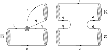
Figure 3: Illustration of rescattering processes of the kind $B^{+}\to\bigl{\{}F_{q}^{(s)}\bigr{\}}\to\pi^{+}K^{0}$. The shaded circle represents insertions of the usual current–current operators $Q_{1,2}^{q}$ ($q\in\{c,u\}$).

4 The Role of Rescattering Processes

In the formalism discussed above, rescattering processes are closely related to the quantity $\rho$ (see Eq. (10)), which is highly CKM-suppressed by $\lambda^{2}R_{b}\approx 0.02$ and receives contributions from penguin topologies with internal top, charm and up quarks, as well as from annihilation topologies. Naïvely, one would expect that annihilation processes play a very minor role, and that penguins with internal top quarks are the most important ones. However, also penguins with internal charm and up quarks lead, in general, to important contributions. $\!{}^{{\bf?}}$ Simple model calculations, performed at the perturbative quark level, do not indicate a significant compensation of the large CKM suppression of $\rho$ through these topologies. However, these crude estimates do not take into account certain rescattering processes, $\!{}^{{\bf?}}$${}^{\mbox{-}}$$\!{}^{{\bf?}}$ which may play an important role and can be divided into two classes: $\!{}^{{\bf?}}$

• $B^{+}\to\{\overline{D^{0}}D_{s}^{+},\,\overline{D^{0}}D_{s}^{\ast+},\,\ldots\}\to\pi^{+}K^{0}$

• $B^{+}\to\{\pi^{0}K^{+},\,\pi^{0}K^{\ast+},\,\ldots\}\to\pi^{+}K^{0}$,

where the dots include also intermediate multibody states. These processes are illustrated in Fig. 3. Here the shaded circle represents insertions of the usual current–current operators

$$\begin{array}[]{rcl}Q_{1}^{q}&=&(\bar{q}_{\alpha}s_{\beta})_{{\rm V-A}}\;(\bar{b}_{\beta}q_{\alpha})_{{\rm V-A}}\\ Q_{2}^{q}&=&(\bar{q}_{\alpha}s_{\alpha})_{{\rm V-A}}\;(\bar{b}_{\beta}q_{\beta})_{{\rm V-A}}\,,\end{array}$$ (22)

where $\alpha$ and $\beta$ are colour indices, and $q\in\{c,u\}$. The rescattering processes (i) and (ii) correspond to $q=c$ and $u$, respectively.

Figure 4: The effect of final-state interactions on $R_{\rm min}$ for $A_{0}=0$. The curves for a given value of $\rho$ correspond to $\theta\in\{0^{\circ},180^{\circ}\}$ and represent the maximal shift from $\rho=0$.

If we look at Fig. 3, we observe that the final-state-interaction (FSI) effects of type (i) can be considered as long-distance contributions to penguin topologies with internal charm quarks, i.e. to the $P_{c}$ amplitude. They may affect BR$(B^{\pm}\to\pi^{\pm}K)$ significantly. On the other hand, the rescattering processes characterized by (ii) result in long-distance contributions to penguin topologies with internal up quarks and to annihilation topologies, i.e. to the amplitudes $P_{u}$ and ${\cal A}$. They play a minor role for BR$(B^{\pm}\to\pi^{\pm}K)$, but may affect assumption (ii) listed in Section 1, thereby leading to a sizeable CP asymmetry, $A_{+}$, as large as ${\cal O}(10\%)$ in this mode. $\!{}^{{\bf?}}$${}^{\mbox{-}}$$\!{}^{{\bf?}}$  The point is as follows: while we would have $\rho\approx 0$ if rescattering processes of type (i) played the dominant role in $B^{+}\to\pi^{+}K^{0}$, or $\rho={\cal O}(\lambda^{2}R_{b})$ if both processes had similar importance, $\rho$ would be as large as ${\cal O}(10\%)$ if the FSI effects characterized by (ii) would dominate $B^{+}\to\pi^{+}K^{0}$ so that $|{\cal P}_{uc}|/|{\cal P}_{tc}|={\cal O}(5)$. This order of magnitude is found in a recent attempt to evaluate rescattering processes of the kind $B^{+}\to\{\pi^{0}K^{+}\}\to\pi^{+}K^{0}$ with the help of Regge phenomenology. $\!{}^{{\bf?}}$  A similar feature is also present in other approaches to deal with these FSI effects. $\!{}^{{\bf?},{\bf?}}$  Therefore, we have arguments that rescattering processes may play an important role.

A detailed study of their impact on the constraints on $\gamma$ arising from the $B^{\pm}\to\pi^{\pm}K$ and $B_{d}\to\pi^{\mp}K^{\pm}$ observables was performed in Ref. 16. While these effects, which are included in the formalism discussed above through the parameter $\kappa$ (see Eq. (20)), are minimal for $\theta\in\{90^{\circ},270^{\circ}\}$ and only of second order, they are maximal for $\theta\in\{0^{\circ},180^{\circ}\}$. In Fig. 4, these maximal effects are shown for various values of $\rho$ in the case of $A_{0}=0$. Looking at this figure, we observe that we have negligibly small effects for $\rho=0.02$, which was assumed in Ref. 6 in the form of point (ii) listed in Section 1. For values of $\rho$ as large as $0.15$, we have an uncertainty for $\gamma_{0}$ (see Eqs. (4) and (5)) of at most $\pm 10^{\circ}$.

Figure 5: Illustration of the strategy to control rescattering effects in $R_{\rm min}$ and the contours in the $\gamma\,$–$\,r$ plane through the decay $B^{\pm}\to K^{\pm}K$ within a simple model (for details, see Ref. 17).

The FSI effects can be controlled through experimental data. A first step towards this goal is provided by the CP asymmetry $A_{+}$. It implies an allowed range for $\rho$, which is given by $\rho_{\rm min}\,\leq\,\rho\,\leq\,\rho^{\rm max}$, with

$$\rho_{\rm min}^{\rm max}=\frac{\sqrt{A_{+}^{2}+\left(1-A_{+}^{2}\right)\sin^{2}\gamma}\pm\sqrt{\left(1-A_{+}^{2}\right)\sin^{2}\gamma}}{|A_{+}|}.$$ (23)

In order to go beyond these constraints, $B^{\pm}\to K^{\pm}K$ decays – the $SU(3)$ counterparts of $B^{\pm}\to\pi^{\pm}K$ – play a key role, allowing us to include the rescattering processes in the contours in the $\gamma\,$–$\,r$ plane and the associated constraints on $\gamma$ completely, as was pointed out in Refs. 16 and 17 (for alternative strategies, see Refs. 10 and 14). As a by-product, this strategy moreover gives an allowed region for $\rho$, and excludes values of $\gamma$ within ranges around $0^{\circ}$ and $180^{\circ}$. It is interesting to note that $SU(3)$ breaking enters in this approach only at the “next-to-leading order” level, as it represents a correction to the correction to the bounds on $\gamma$ arising from rescattering processes. Moreover, this strategy also works if the CP asymmetry $A_{+}$ arising in $B^{+}\to\pi^{+}K^{0}$ should turn out to be very small. In this case, there may also be large rescattering effects, which would then not be signalled by sizeable CP violation in this channel.

Following Ref. 17, this approach to control the FSI effects is illustrated in Fig. 5 by showing the contours in the $\gamma\,$–$\,r$ plane and the dependence of $R_{\rm min}$ on the CKM angle $\gamma$. Here the simple model advocated by the authors of Refs. 12 and 13 was used to obtain values for the $B\to\pi K$, $KK$ observables by choosing a specific set of input parameters (for details, see Ref. 17). The value of $R=0.83$ arising in this case is represented in Fig. 5 by the dotted line. It is an easy exercise to read off the corresponding allowed range for $\gamma$ from this figure.

Since the “short-distance” expectation for the combined branching ratio BR$(B^{\pm}\to K^{\pm}K)$ is ${\cal O}(10^{-6})$, $\!{}^{{\bf?}}$ experimental studies of $B^{\pm}\to K^{\pm}K$ appear to be difficult. These modes have not yet been observed, and only upper limits for BR$(B^{\pm}\to K^{\pm}K)$ are available. $\!{}^{{\bf?},{\bf?}}$  However, rescattering effects may enhance this quantity significantly, and could thereby make $B^{\pm}\to K^{\pm}K$ measurable at future $B$-factories. $\!{}^{{\bf?},{\bf?}}$  Another important indicator of large FSI effects is provided by $B_{d}\to K^{+}K^{-}$ decays, $\!{}^{{\bf?}}$ for which stronger experimental bounds already exist. $\!{}^{{\bf?},{\bf?}}$

Although $B^{\pm}\to K^{\pm}K$ decays allow us to determine the shift of the contours in the $\gamma\,$–$\,r$ plane arising from rescattering processes, they do not allow us to take into account these effects also in the determination of $\gamma$, requiring some knowledge on $r$, in contrast to the bounds on $\gamma$. As we have already noted, this quantity is not just the ratio of a “tree” to a “penguin” amplitude, which is the usual terminology, but has a rather complex structure and may in principle be considerably affected by FSI effects. However, if future measurements of BR$(B^{\pm}\to K^{\pm}K)$ and BR$(B_{d}\to K^{+}K^{-})$ should not show a significant enhancement with respect to the “short-distance” expectations of ${\cal O}(10^{-6})$ and ${\cal O}(10^{-8})$, respectively, and if $A_{+}$ should not be in excess of ${\cal O}(1\%)$, a future theoretical accuracy of $r$ as small as ${\cal O}(10\%)$ may be achievable.

Figure 6: The effect of electroweak penguins on $R_{\rm min}$ for $|A_{0}|=0.2$. The curves for a given value of $\epsilon$ correspond to $\Delta\in\{0^{\circ},180^{\circ}\}$ and represent the maximal shift from $\epsilon=0$.

5 The Role of Electroweak Penguins

The modification of $R_{\rm min}$ through EW penguin topologies is described by $\kappa=1+2\,\epsilon\,\cos\Delta+\epsilon^{2}$. These effects are minimal and only of second order in $\epsilon$ for $\Delta\in\{90^{\circ},270^{\circ}\}$, and maximal for $\Delta\in\{0^{\circ},180^{\circ}\}$. In the case of $\Delta=0^{\circ}$, which is favoured by “factorization”, the bounds on $\gamma$ get stronger, excluding a larger region around $\gamma=90^{\circ}$, while they are weakened for $\Delta=180^{\circ}$. In Fig. 6, the maximal EW penguin effects are shown for $|A_{0}|=0.2$ and for various values of $\epsilon$. The EW penguins are “colour-suppressed” in the case of $B^{+}\to\pi^{+}K^{0}$ and $B^{0}_{d}\to\pi^{-}K^{+}$; estimates based on simple calculations performed at the perturbative quark level, where the relevant hadronic matrix elements are treated within the “factorization” approach, typically give $\epsilon={\cal O}(1\%)$. $\!{}^{{\bf?}}$  These crude estimates may, however, underestimate the role of these topologies. $\!{}^{{\bf?},{\bf?}}$

An improved theoretical description of the EW penguins is possible, using the general expressions for the corresponding four-quark operators and performing appropriate Fierz transformations. Following these lines, $\!{}^{{\bf?}}$ we arrive at the expression

$$\frac{\epsilon}{r}\,e^{i(\Delta-\delta)}\approx\frac{3}{2\lambda^{2}R_{b}}\left[\frac{C_{1}^{\prime}(\mu)C_{10}(\mu)-C_{2}^{\prime}(\mu)C_{9}(\mu)}{C_{2}^{\prime 2}(\mu)-C_{1}^{\prime 2}(\mu)}\right]a\,e^{i\omega}$$ (24)

with $C_{1}^{\prime}(\mu)\equiv C_{1}(\mu)+3\,C_{9}(\mu)/2$ and $C_{2}^{\prime}(\mu)\equiv C_{2}(\mu)+3\,C_{10}(\mu)/2$, where $C_{1,2}(\mu)$ are the Wilson coefficients of the current–current operators specified in Eq. (22), and $C_{9,10}(\mu)$ those of the EW penguin operators

$$\begin{array}[]{rcl}Q_{9}&=&\frac{3}{2}(\bar{b}_{\alpha}s_{\alpha})_{{\rm V-A}}\sum\limits_{q=u,d,c,s,b}c_{q}\,(\bar{q}_{\beta}q_{\beta})_{{\rm V-A}}\\ Q_{10}&=&\frac{3}{2}(\bar{b}_{\alpha}s_{\beta})_{{\rm V-A}}\sum\limits_{q=u,d,c,s,b}c_{q}\,(\bar{q}_{\beta}q_{\alpha})_{{\rm V-A}}\,.\end{array}$$ (25)

The combination of Wilson coefficients in Eq. (24) is essentially renormalization-scale-independent and changes only by ${\cal O}(1\%)$ when evolving from $\mu=M_{W}$ down to $\mu=m_{b}$. Employing $R_{b}=0.36$ and typical values for the Wilson coefficients yields $\!{}^{{\bf?}}$

$$\frac{\epsilon}{r}\,e^{i(\Delta-\delta)}\approx 0.75\times a\,e^{i\omega}.$$ (26)

The quantity $a\,e^{i\omega}$ is given by

$$a\,e^{i\omega}\equiv\frac{a_{2}^{\rm eff}}{a_{1}^{\rm eff}}\,,$$ (27)

where $a_{1}^{\rm eff}$ and $a_{2}^{\rm eff}$ correspond to a generalization of the usual phenomenological colour factors $a_{1}$ and $a_{2}$ describing the “strength” of colour-suppressed and colour-allowed decay processes, respectively. $\!{}^{{\bf?}}$  Comparing experimental data on $B^{-}\to D^{(\ast)0}\pi^{-}$ and $\overline{B^{0}_{d}}\to D^{(\ast)+}\pi^{-}$, as well as on $B^{-}\to D^{(\ast)0}\rho^{-}$ and $\overline{B^{0}_{d}}\to D^{(\ast)+}\rho^{-}$ decays gives $a_{2}/a_{1}={\cal O}(0.25)$, where $a_{1}$ and $a_{2}$ are – in contrast to $a_{1}^{\rm eff}$ and $a_{2}^{\rm eff}$ – real quantities, and their relative sign is found to be positive. For $a=0.25$, we obtain a value of $\epsilon/r$ that is larger than the “factorized” result

$$\left.\frac{\epsilon}{r}\,e^{i(\Delta-\delta)}\right|_{\rm fact}=\,0.06$$ (28)

by a factor of 3. A detailed study of the effects of the EW penguins described by Eq. (24) on the strategies to probe the CKM angle $\gamma$ discussed in Section 3 was performed in Ref. 16. There it was also pointed out that a first step towards the experimental control of the “colour-suppressed” EW penguin contributions to the $B\to\pi K$ amplitude relations (12) and (13) is provided by the decay $B^{+}\to\pi^{+}\pi^{0}$. More refined strategies will certainly be developed in the future, when better experimental data become available.

6 Probing $\gamma$ with $B_{s}\to K\overline{K}$ Decays

In this section, we focus on the modes $B_{s}\to K^{0}\overline{K^{0}}$ and $B_{s}\to K^{+}K^{-}$, which are the $B_{s}$ counterparts of the $B_{u,d}\to\pi K$ decays discussed above, where the up and down “spectator” quarks are replaced by a strange quark. Because of the expected large $B^{0}_{s}$–$\overline{B^{0}_{s}}$ mixing parameter $x_{s}\equiv\Delta M_{s}/\Gamma_{s}={\cal O}(20)$, experimental studies of CP violation in $B_{s}$ decays are regarded as being very difficult. In particular, an excellent vertex resolution system is required to keep track of the rapid oscillatory $\Delta M_{s}t$ terms arising in tagged $B_{s}$ decays. These terms cancel, however, in the untagged $B_{s}$ decay rates defined by

$$\Gamma[f(t)]\equiv\Gamma(B_{s}^{0}(t)\to f)\,+\,\Gamma(\overline{B^{0}_{s}}(t)\to f)\,,$$ (29)

where one does not distinguish between initially, i.e. at time $t=0$, present $B^{0}_{s}$ and $\overline{B^{0}_{s}}$ mesons. In this case, the expected sizeable width difference $\!{}^{{\bf?}}$ $\Delta\Gamma_{s}\equiv\Gamma_{H}^{(s)}-\Gamma_{L}^{(s)}$ between the mass eigenstates $B_{s}^{H}$ (“heavy”) and $B_{s}^{L}$ (“light”) of the $B_{s}$ system may provide an alternative route to explore CP violation. $\!{}^{{\bf?}}$  Several strategies were proposed to extract CKM phases from experimental studies of such untagged $B_{s}$ decays. $\!{}^{{\bf?}}$${}^{\mbox{-}}$$\!{}^{{\bf?}}$

In Ref. 24, it was pointed out that the modes $B_{s}\to K^{0}\overline{K^{0}}$ and $B_{s}\to K^{+}K^{-}$ probe the CKM angle $\gamma$. Their decay amplitudes take a form completely analogous to Eqs. (12) and (13), and the corresponding untagged decay rates can be expressed as follows: $\!{}^{{\bf?}}$

$$\Gamma[K^{0}\overline{K^{0}}(t)] = R_{L}\,e^{-\Gamma_{L}^{(s)}t}+R_{H}\,e^{-\Gamma_{H}^{(s)}t}$$ (30)

$$\Gamma[K^{+}K^{-}(t)] = \Gamma[K^{0}\overline{K^{0}}(0)]\left[a\,e^{-\Gamma_{L}^{(s)}t}+b\,e^{-\Gamma_{H}^{(s)}t}\right].\qquad\mbox{}$$ (31)

Since we have $a+b=R_{s}$, where $R_{s}$ corresponds to the ratio $R$ of the combined $B\to\pi K$ branching ratios (see Eq. (3)), bounds on $\gamma$ similar to those discussed in Sections 1 and 3 can also be obtained from the untagged $B_{s}\to K\overline{K}$ observables. Moreover, a comparison of $R$ and $R_{s}$ provides valuable insights into $SU(3)$ breaking.

A closer look shows, however, that it is possible to derive more elaborate bounds from the untagged $B_{s}\to K\overline{K}$ rates: $\!{}^{{\bf?}}$

$$\frac{\left|\,1-\sqrt{a}\,\right|}{\sqrt{b}}\leq|\cot\gamma\,|\leq\frac{1+\sqrt{a}}{\sqrt{b}}\,,$$ (32)

corresponding to the allowed range

$$\gamma_{1}\leq\gamma\leq\gamma_{2}\quad\lor\quad 180^{\circ}-\gamma_{2}\leq\gamma\leq 180^{\circ}-\gamma_{1}$$ (33)

with

$$\gamma_{1}\equiv\mbox{arccot}\left(\frac{1+\sqrt{a}}{\sqrt{b}}\right),\quad\gamma_{2}\equiv\mbox{arccot}\left(\frac{\left|\,1-\sqrt{a}\,\right|}{\sqrt{b}}\right).$$ (34)

Besides a sizeable value of $\Delta\Gamma_{s}$ and non-vanishing observables $a$ and $b$, the bound (32) does not require any constraint on these observables such as $R_{s}=a+b<1$, which is needed for Eqs. (4) and (5) to become effective.

As in the $B\to\pi K$ case, the theoretical accuracy of these constraints, which make use only of the general amplitude structure arising within the Standard Model and of the $SU(2)$ isospin symmetry of strong interactions, is also limited by certain rescattering processes and contributions arising from EW penguins. In Eq. (32), these effects are neglected for simplicity. The completely general formalism, taking also into account these effects, is derived in Ref. 26, where also strategies to control them through experimental data are discussed.

In order to go beyond these constraints and to determine $\gamma$ from the untagged $B_{s}\to K\overline{K}$ observables, the magnitude of an amplitude $T_{s}$, which corresponds to $T$ (see Eq. (15)), has to be fixed, leading to hadronic uncertainties similar to those in the $B\to\pi K$ case. Such an input can be avoided by considering the contours in the $\gamma\,$–$\,r_{(s)}$ and $\gamma\,$–$\,\cos\delta_{(s)}$ planes, and applying the $SU(3)$ flavour symmetry to relate $r_{s}$ to $r$ and $\cos\delta_{s}$ to $\cos\delta$, respectively. $\!{}^{{\bf?}}$ The contours in the $\gamma\,$–$\,r_{(s)}$ plane are illustrated in Fig. 7. Using the formalism presented in Refs. 16, 17 and 26, rescattering and EW penguin effects can be included in these contours. As a “by-product”, also values for the hadronic quantities $r_{(s)}$ and $\cos\delta_{(s)}$ are obtained, which are of special interest to test the factorization hypothesis.

Figure 7: The contours in the $\gamma\,$–$\,r_{(s)}$ plane for $a=0.60$, $b=0.15$ and $\rho_{s}=0.15$, $\epsilon_{s}=0$. The $B\to\pi K$ contours correspond to $R=0.75$, $A_{0}=0.2$ and $\rho=\epsilon=0$.

Provided a tagged, time-dependent measurement of $B_{s}\to K^{0}\overline{K^{0}}$ and $B_{s}\to K^{+}K^{-}$ can be performed, $\!{}^{{\bf?}}$ it would be possible to extract $\gamma$ in such a way that rescattering effects are taken into account “automatically”. $\!{}^{{\bf?}}$  To this end, the $B_{s}\to K\overline{K}$ observables are sufficient, and the theoretical accuracy of $\gamma$ would only be limited by EW penguins. Let me finally note that the $B_{s}\to K\overline{K}$ decays represent also an interesting probe for certain scenarios of physics beyond the Standard Model. $\!{}^{{\bf?}}$

7 Conclusions

On the long and winding road towards the extraction of the CKM angle $\gamma$, the decays $B^{\pm}\to\pi^{\pm}K$ and $B_{d}\to\pi^{\mp}K^{\pm}$ are expected to play an important role. An accurate measurement of these modes, as well as of $B\to KK$ and $B\to\pi\pi$ decays to control rescattering and EW penguin effects, is therefore an important goal of the future $B$-factories. At present, data for these decays are already starting to become available, and the coming years will certainly be very exciting. The modes $B_{s}\to K^{0}\overline{K^{0}}$ and $B_{s}\to K^{+}K^{-}$ also offer interesting strategies to probe the CKM angle $\gamma$. Here the width difference $\Delta\Gamma_{s}$ may provide an interesting tool to accomplish this task. In order to investigate $B_{s}$ decays, experiments at hadron machines appear to be most promising.

References

References

- [1] R. Fleischer, Int. J. Mod. Phys. A12, 2459 (1997).
- [2] R. Fleischer, Phys. Lett. B365, 399 (1996).
- [3] M. Gronau and J.L. Rosner, Phys. Rev. D57, 6843 (1998).
- [4] F. Würthwein and P. Gaidarev, preprint CALT-68-2153 (1997) [hep-ph/9712531].
- [5] CLEO Collaboration (R. Godang et al.), Phys. Rev. Lett. 80, 3456 (1998).
- [6] R. Fleischer and T. Mannel, Phys. Rev. D57, 2752 (1998).
- [7] CLEO Collaboration (M. Artuso et al.), preprint CLEO CONF 98-20, ICHEP98 858; J. Alexander, these proceedings.
- [8] A. Buras, preprint TUM-HEP-299/97 (1997) [hep-ph/9711217].
- [9] Y. Grossman et al., Nucl. Phys. B511, 69 (1998).
- [10] A.J. Buras, R. Fleischer and T. Mannel, preprint CERN-TH/97-307 (1997) [hep-ph/9711262], to appear in Nucl. Phys. B.
- [11] L. Wolfenstein, Phys. Rev. D52, 537 (1995).
- [12] J.-M. Gérard and J. Weyers, preprint UCL-IPT-97-18 (1997) [hep-ph/9711469].
- [13] M. Neubert, Phys. Lett. B424, 152 (1998).
- [14] A.F. Falk et al., Phys. Rev. D57, 4290 (1998).
- [15] D. Atwood and A. Soni, Phys. Rev. D58, 036005 (1998).
- [16] R. Fleischer, preprint CERN-TH/98-60 (1998) [hep-ph/9802433], to appear in Eur. Phys. J. C.
- [17] R. Fleischer, preprint CERN-TH/98-128 (1998) [hep-ph/9804319], to appear in Phys. Lett. B.
- [18] L. Wolfenstein, Phys. Rev. Lett. 51, 1945 (1983).
- [19] A.J. Buras and R. Fleischer, Phys. Lett. B341, 379 (1995); R. Fleischer, Phys. Lett. B341, 205 (1994); M. Ciuchini et al., Nucl. Phys. B501, 271 (1997).
- [20] For a recent study, see A. Ali, G. Kramer and C.-D. Lü, preprint DESY 98-041 (1998) [hep-ph/9804363]; A. Ali, these proceedings.
- [21] M. Gronau and J.L. Rosner, preprint EFI-98-23 (1998) [hep-ph/9806348].
- [22] For a recent calculation of , see M. Beneke et al., preprint CERN-TH/98-261 (1998) [hep-ph/9808385].
- [23] I. Dunietz, Phys. Rev. D52, 3048 (1995).
- [24] R. Fleischer and I. Dunietz, Phys. Rev. D55, 259 (1997).
- [25] R. Fleischer and I. Dunietz, Phys. Lett. B387, 361 (1996).
- [26] R. Fleischer, preprint CERN-TH/97-281 (1997) [hep-ph/9710331], to appear in Phys. Rev. D.
- [27] C.S. Kim, D. London and T. Yoshikawa, Phys. Rev. D57, 4010 (1998).