HD–THEP 98–40

Time evolution of observables out of thermal equilibrium.

Abstract

We propose a new approximation–technique to deal with the exact macroscopic integro–differential evolution equations of statistical systems which self–consistently accounts for dissipative effects. Concentrating on one and two point equal–time correlators, we develop the self–consistent method and apply it to a scalar field theory with quartic self–interaction. We derive the effective equations of motion and the corresponding macroscopic effective Hamiltonian. Non–locality in time appears in a natural way necessary to account for entropy generating processes.

I Introduction

The question of how and if a statistical infinite dimensional quantum system thermalises is one of the fundamental problems of statistical mechanics, and has recently attracted much attention in connection with problems in cosmology and relativistic heavy ion physics. We discussed some related issues in a recent work [1] for a zero dimensional quantum mechanical model. There, we concluded that a safe and consistent method to investigate on time evolution of macroscopic observables is to apply the projection operator technique. In this work, we systematically apply the new self–consistent approximation technique anticipated in [1] to a scalar field theory with quartic self–interaction. For systematic reasons, let us therefore briefly review the line of arguments leading to that concept.

In statistical theory, a level of observation is defined by a set of Hermitian so–called relevant operators the expectation values of which are the macroscopic observables of the ensemble under consideration. The dynamics is defined by the microscopic Hamiltonian which enters in the exact integro–differential equations of motion for the macroscopic observables, as derived by the projection–operator technique [2]. These equations solve the complete BBGKY-hierarchy in integral form and are closed in the observables under consideration. Correlators not expressible in terms of the basic observables are eliminated by the projection procedure but leave their imprints implicitly in the defining equation of a projected evolution operator. The problem of resolving the infinite set of differential equations of the BBGKY–hierarchy, and subsequent reduction to the macroscopically relevant quantities, has thus been converted into approximating that operator in a self–consistent way. Only in some particular cases, as for effectively non–interacting systems defined by a Hamiltonian which contain polynomials of at most second order in position and momentum operators, the projected time evolution operator can be integrated without explicit dependence on projectors. A side–condition for exact integrability is that also the level of observation must be chosen to be at most of second order (quadratic level of observation). The physical reason for exact integrability is dynamical closure, i.e. the fact that time evolution driven by effectively non–interacting Hamiltonians does not lead out of the linear space spanned by the operators of a quadratic level of observation. Typical examples of this type are time dependent mass–parameters or QED without quantized fermions, but including classical external sources.

For the interacting case, the expansion of the projected evolution operator into a coupling parameter labeling the interaction part is discussed extensively in the literature [2]. However, that expansion scheme turns out to be inconsistent with the projected dynamics at second order even when we introduce an effective quadratic micro-dynamical Hamiltonian and expand the projected time evolution operator around it. That was demonstrated explicitly in a zero-dimensional toy model recently [1]. The break–down of that kind of expansions becomes apparent if one integrates the system for times large compared to the inverse coupling of the interaction part. The physical reason for that may best be illustrated by considering the uncertainty product expressible in terms of the quadratic observables. Even for effectively non–interacting Hamiltonians with arbitrary time dependent coefficients, the uncertainty – which essentially is the volume of phase space cells – is an exact constant of motion. However, the dissipative part of the equations of motion for the observables does not respect constant uncertainty, and evolves it to numerically large values at secular time scales. On the other hand, increasing uncertainty and increasing phase space volume of the corresponding macroscopic dynamics is an essential feature of non–equilibrium statistical systems. Moreover, the uncertainty product is directly related to the relevant entropy of a quadratic level of observation. We concluded that any effective microscopic Hamiltonian is intrinsically incompatible with time variant entropy and cannot be used to approximate the projected evolution operator. One necessarily has to generalize to an effective Liouvillian acting in the space of relevant operators and expand around its associated so–called reduced time evolution operator.

The task of the present investigation is to derive the effective equations of motion by approximating the projected evolution operator by its reduced counterpart to the first non-trivial order. We also construct the corresponding effective Hamiltonian which generates the macroscopic equations of motion.

II Definition of the problem

(i) A mixed state of a quantum system (configuration), both in zero dimensional quantum mechanics as well as in quantum field theory, is described by a density operator, which, in order to allow a probability interpretation, must be a hermitian trace-class operator with positive eigenvalues. It is an intrinsic feature of quantum systems that the density matrix is fictive in the sense that only its diagonal elements correspond to physical probabilities, the other dependencies being phases which enter in expectation values via interference effects. Alternatively, one may characterize a configuration by the expectation values of hermitian operators. A generic set of those representing a complete set of observables is given by the mutually orthogonal hermitian projectors constructed from the eigenvectors of the density matrix. A complete set of (not necessarily commuting) observables contains all information about the density matrix such that any observable can be expressed in terms of the complete set.

(ii) The system may be assigned a dynamical structure. Motion is defined as a sequence of possible states having a constant expectation value of the Hamiltonian operator, the energy of the configuration. Quantum mechanical time parameterizes those configurations which are assumed to have time–independent probabilities and phases for autonomous systems. The time evolution generated by the micro-dynamical Hamiltonian can be expressed by first order differential operator–equations in time for the density matrix (von Neumann equation) in the Schrödinger representation,

$$i\frac{d}{dt}\rho(t)=[H,\rho(t)],$$ (1)

together with an initial condition $\rho(0)$. Hermitian Hamilton–operators generate unitary time evolution which in turn is necessary to allow for a probability interpretation. Once the problem of time evolution of the mixed state is solved for a given initial configuration, observables can be calculated as expectation values from the evolved density matrix.

(iii) The statistical description of a system is based on a reduction procedure selecting an in general much smaller number of (macroscopic) observed quantities out of the complete set of observables. This subset defines the level of observation (description), characterized by the set of relevant operators ${\cal E}=\{{\cal F}_{\nu}\}.$ The process of reduction from the density operator to the set of the so–called relevant quantities in general involves loss of information. Here, we will concentrate on levels of observation that once chosen, will be kept fixed during time evolution. That constraint can be relaxed too if necessary [3].

(iv) The reduction can be dynamically trivial if it commutes with time evolution. In that case of dynamical closure, the Liouvillian maps the operators of the level of description on a linear combination of them. The observables of a level of description at a certain time are sufficient to determine them at any time and evolution induces neither information gain nor information loss at the level of observation, the associated entropy being constant. On account of the canonical commutation relation, the most general Hamiltonian admitting a finite dimensional dynamically closed level of observation can contain constant, linear and quadratic expressions in position and momentum operators. The corresponding dynamically closed sets of observables correspond to sums of polynomials of finite order in the canonical operators. If the reduction is non-trivial, one can extend the level of observation to render it trivial. That may involve an infinite number of operators in which case the system is a truly interacting one, and the only dynamically closed set of operators corresponds to a complete set of observables.

(v) For truly interacting dynamical systems, the complete initial density matrix influences observables at later times. Its definition calls for an additional principle to construct it from the reduced set of initial data. Information theory proposes to apply Shannon’s theory of entropy [4] to that physical problem. Jaynes’ principle of maximum entropy [5] fixes the generalized canonical density operator as initial condition. It can be shown not to contain more information than the initial set of observables. We want to point out that this choice is the statistically most probable, but the underlying concept of ensemble averages of identical systems evolving from variant initial preparations does not imply actual the preparation of the physical system in that state.

The reduced description of a quantum system is achieved by passing from the density matrix to a statistical operator characteristic for the ensemble under consideration. The best guess for that operator compatible with the principle of maximum entropy has the functional form

$${\cal R}=\exp({-\mu_{\nu}{\cal F}_{\nu}}).$$

It contains exactly the same amount of information on the system as the statistical observables $g_{\nu}=\mbox{tr}\left(\rho{\cal F}_{\nu}\right)=\mbox{tr}\left({\cal R}{\cal F}_{\nu}\right)$, and maximizes the relevant entropy functional of the level of observation,

$$S_{{\cal E}}=-\mbox{tr}\left({\cal R}\log{\cal R}\right)=\mu_{\nu}g_{\nu}.$$ (2)

Reducing the description of a quantum mixed state to the evolution of the accompanying statistical operator ${\cal R}$ requires to derive a modified evolution equation which does not lead out of the level of observation. The problem basically boils down to introducing suitable projection operators and the study of their associated time evolution.

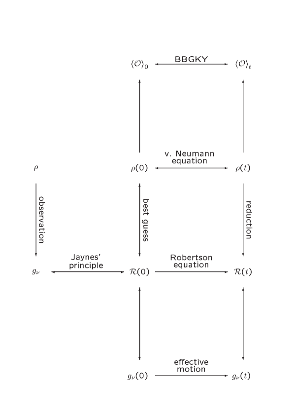
FIG. 1.: Overview of relations on time evolution of mixed states and statistical time evolution. The arrows indicate the sense of deduction.

An overview of the systematics is given in Fig. (1). Here, we adopt the Robertson equation approach. Alternatively, one may solve the BBGKY–hierarchy which, however, is problematic since it involves an ad hoc truncation procedure. Problems with that approach have been discussed extensively elsewhere [1].

III Projection Operator Technique

We briefly review some basic terms of the projection operator approach [2, 3] serving as starting point of the present investigation. There, one defines the level of observation by the finite set of Hermitian operators ${\cal E}=\{{\cal F}_{\nu}\}$ including ${\cal F}_{0}=\mbox{1 1 }$ for convenience. The accompanying canonical density operator defined by ${\cal R}(t)=\exp(-\mu_{\nu}(t){\cal F}_{\nu})$ contains time dependent Lagrange multipliers $\mu_{\nu}(t)$ which are functions of $g_{\nu}(t)$ such that $g_{\nu}(t)=\mbox{tr}\left({\cal F}_{\nu}\rho(t)\right)=\mbox{tr}\left({\cal F}_{\nu}{\cal R}(t)\right)$. We emphasize that other than the density matrix $\rho(t)$, ${\cal R}(t)$ in general does not evolve according to a Schrödinger equation.

For the corresponding operator expectation values $g_{\nu}(t)$, the closed exact equation (Robertson equation) of motion is found to read

$$\frac{d}{dt}g_{\nu}(t)=-i\,\mbox{tr}\left({\cal F}_{\nu}L\circ{\cal R}(t)\right)$$ (3)

$$\quad-\int_{0}^{t}\!dt^{\prime}\,\mbox{tr}\left({\cal F}_{\nu}L\circ T(t,t^{\prime})\circ Q(t^{\prime})\circ L\circ{\cal R}(t^{\prime})\right).$$ (4)

Here $L$ stands for the Liouvillian induced by the micro-dynamical Hamiltonian, and the action of $L$ on some operator ${\cal X}$ is defined by $L\circ{\cal X}=[H,{\cal X}]$.

The r.h.s. of (4) introduces two new symbols which call for further explanation. The projector $Q(t)$ is defined by

$$\mbox{tr}({\cal O}_{1}Q(t)\circ{\cal O}_{2})=\mbox{tr}({\cal O}_{1}{\cal O}_{2})-\frac{\partial\mbox{tr}({\cal O}_{1}{\cal R}(t))}{\partial g_{\nu}(t)}\,\mbox{tr}({\cal F}_{\nu}{\cal O}_{2}),$$ (5)

for any pair of operators ${\cal O}_{1},{\cal O}_{2}$. In the particular case of ${\cal O}_{1}$ being in the linear space of the level of observation ${\cal E}$, the rhs of Eq. (5) vanishes.

The non-unitary projected evolution operator $T(t,t^{\prime})$ is a solution of

$$\frac{\partial}{\partial t}T(t,t^{\prime}) = -iQ(t)\circ L\circ T(t,t^{\prime})\qquad\mbox{and}$$ (6)

$$\frac{\partial}{\partial t^{\prime}}T(t,t^{\prime}) = iT(t,t^{\prime})\circ Q(t^{\prime})\circ L$$ (7)

with initial condition $T(t,t)=1$. It will turn out to be the key problem to construct this operator from its definition for the particular Hamiltonian under consideration. Then, all trace expressions at the r.h.s. of (4) can at least in principle be expressed in terms of the $g_{\nu}$, and the system is a closed integro-differential equation in the c-number expectation values.

In this investigation, we will complete ${\cal E}$ such that the action of the Hamiltonian induced Liouvillian can be split into $L=L_{0}+L_{I}$, and the free part be dynamically closed with respect to the level of observation, $L_{0}\circ{\cal F}_{\nu}=[H_{0},{\cal F}_{\nu}]=\Omega_{\nu\mu}{\cal F}_{\mu}$. In that case, in the integral part of Eq. (4), the complete Liouvillian can be replaced by $L_{I}$.

Expectation values of operators which cannot be represented as linear combinations of the level of observation get additional contributions to their ${\cal R}$-averages,

$$\mbox{tr}({\cal O}\rho(t)) = \mbox{tr}\left({\cal O}{\cal R}(t)\right)$$ (8)

$$- i\int_{0}^{t}dt^{\prime}\mbox{tr}\left({\cal O}T(t,t^{\prime})\circ Q(t^{\prime})\circ L\circ{\cal R}(t^{\prime})\right),$$ (9)

where again the dynamically closed part in $L$ does not contribute to the integral.

IV Projected evolution

The key problem is to find a consistent approximation scheme to solve the defining equation for the projected evolution operator $T(t,t^{\prime})$. That scheme — order by order – must (i) be compatible with the Robertson equation and (ii) conserve exact constants of motion. In particular, the expectation value of the Hamiltonian operator being a generic constant of motion must be conserved which is a non–trivial condition since, due to relation (9), that generally involves integral terms non–local in time. The query for a consistent approximation scheme naturally raises the question whether there exists an effective micro-canonical Hamiltonian which may serve as a zeroth–order approximation being a staring point of an expansion.

A fist approach to that problem is to study the small $\lambda$ expansion of $H=H_{0}+\lambda H_{I}$. If one evaluates the corresponding expressions to second order in the coupling and solves the resulting system of integro–differential equations of motion, one finds that the expansion breaks down at typical secular time scales of the order $t\sim 1/\lambda$ [1].

An improvement of that expansion scheme in equilibrium theory can be achieved by resummation. In our case, that amounts to introduce an effective Hamiltonian. In particular, one may try to make an quadratic Ansatz of the form

$$H_{\mbox{eff}}=a(t;x,y)\Pi(x)\Pi(y)+b(t;x,y)\Phi(x)\Phi(y)+\ldots$$

and determine the time dependent coefficients by self–consistency requirements. However, it turns out that even that improved scheme fails to meet the consistency conditions (i,ii) at secular time scales [1]. The physical reason for that is the presence of memory effects. In particular, although the effective Hamiltonian correctly describes time evolution for short times $t\ll 1/\lambda$ in an appropriate way, the time evolved quantity $H_{\mbox{eff}}$ does not coincide with effective Hamiltonian constructed by the consistency requirements at later times. We conclude that only the enveloping dynamics is an effective Hamiltonian one. Furthermore, effective Hamiltonian dynamics automatically gives rise to an additional constant of motion related to the uncertainty product of the configuration. On account of the uncertainty–entropy relation for quadratic observables, that results in conservation of the relevant entropy contradicting constant information loss inherent in the dissipative time evolution of statistical systems. Also, locality in time conflicts with the presence of memory terms, which get important at large time scales. Third, an effective Hamiltonian automatically induces a unitary effective time evolution operator which again conserves observable information. The conclusion is that there generally exists no effective micro-dynamical Hamiltonian dynamics which is compatible with the Robertson–equation and conservation of energy. We thus have to completely abandon the query for micro-dynamical Hamiltonians in favor of a the more general concept of Liouvillian dynamics.

The key idea is to formally introduce an effective evolution operator which evolves the accompanying statistical operator ${\cal R}(t)$ in a form–invariant way and expand the projected evolution operator around that reduced time evolution.

The reduced time evolution super–operator ${\cal V}(t,t^{\prime})$ is uniquely defined by two demands. Firstly, it does not lead out of the linear space of the relevant operators (observables). Secondly, it evolves the statistical operator,

$${\cal R}(t)={\cal V}(t,t^{\prime})\circ{\cal R}(t^{\prime}).$$ (10)

That condition already is very restrictive. Due to the particular form of the accompanying statistical operator, the differentiated equation suggests to write a solution as a time-ordered exponential

$${\cal V}(t,t^{\prime})={\cal T}\exp\left(-i\int_{t^{\prime}}^{t}d\tau\hat{L}(\tau)\circ{}\right).$$ (11)

Since the derivative $\partial_{t}$ obeys the Leibnitz product–rule, the effective Liouvillian–Operator $\hat{L}(t)$ has to have the algebraic property of a derivation, $\hat{L}(t)\circ(AB)=(\hat{L}(t)\circ A)B+A(\hat{L}(t)\circ B)$. We want to point out that in general this Liouvillian is not an anti–hermitian operator, $\hat{L}\neq-\hat{L}^{\dagger}$ and thus cannot be cast as a commutator with some effective Hamiltonian, $\hat{L}\neq[\hat{H},.\,].$

Furthermore, on account of linearity in the level of observation, the reduced time evolution can be expressed in terms of a matrix evolution operator, ${\cal V}(t,t^{\prime})\circ{\cal F}_{\alpha}={\cal V}_{\alpha\beta}(t,t^{\prime}){\cal F}_{\beta}$. The reduced time evolution operator still possesses the property of transitivity, ${\cal V}(t,t^{\prime})\circ{\cal V}(t^{\prime},t^{\prime\prime})={\cal V}(t,t^{\prime\prime})$.

In practical calculations, it turns out to be convenient to act with the reduced time evolution operator to its left which amounts to define the adjoint action induced by the trace as inner product by

$$\mbox{tr}\left({\cal O}{\cal V}(t,t^{\prime})\circ{\cal R}(t^{\prime})\right) = \mbox{tr}\left(({\cal V}^{\dagger}(t,t^{\prime})\circ{\cal O}){\cal R}(t^{\prime})\right)$$ (12)

$$= \mbox{tr}\left({\cal O}(t,t^{\prime}){\cal R}(t^{\prime})\right).$$ (13)

The adjoint evolved operator ${\cal O}(t,t^{\prime})$ is the generalization of the free Heisenberg operator to ${\cal O}$ for non–Hamiltonian time evolution. Due to the particular properties of ${\cal V}(t,t^{\prime})$, one can also express time evolution of the generalized Heisenberg operators of the basis by means of a matrix multiplication, ${\cal F}_{\alpha}(t,t^{\prime})={\cal V}^{\dagger}(t,t^{\prime})\circ{\cal F}_{\alpha}={\cal V}^{\dagger}_{\alpha\beta}(t,t^{\prime}){\cal F}_{\beta}.$ The matrix elements are restricted by the conditions

$$g_{\alpha}(t)={\cal V}^{\dagger}_{\alpha\beta}(t,t^{\prime})g_{\beta}(t^{\prime}).$$ (14)

In addition to that, the property

$${\cal V}^{\dagger}(t,t^{\prime})\circ({\cal F}_{\alpha}{\cal F}_{\beta})=\left({\cal V}^{\dagger}(t,t^{\prime})\circ{\cal F}_{\alpha}\right)\left({\cal V}^{\dagger}(t,t^{\prime})\circ{\cal F}_{\beta}\right)$$ (15)

which is a direct consequence of $\hat{L}(t)$ being a derivation, further restricts the number of independent elements in the evolution matrix if some symmetrised products $\{{\cal F}_{\alpha},{\cal F}_{\beta}\}$ are also in the operator basis of the level of observation. In general, however, those conditions are not sufficient to fix the evolution matrix completely.

The self–consistent method now requires to expand the projected evolution operator in terms of the reduced time evolution operator. It is part of our strategy to exploit the remaining freedom in the evolution matrix to satisfy consistency with the Robertson evolution equations, and possible conserved quantities. As will be shown in the case of the local and bilocal equal–time correlators as observables, that fixes the dissipative evolution matrix in a consistent way.

V Reduced evolution operator for one and two point correlators

In order to define the ensemble, a particular set of observables must be chosen. Among various choices of the level of observation, the special case of quadratic observables plays a particular rôle. This set of Hermitian operators that can be constructed out of the field operators and its canonically conjugate momentum, $\{\mbox{1 1 }$, $\Phi(x)$, $\Pi(x)$, $\Phi(x)\Phi(y)$, $W(x,y)=\Phi(x)\Pi(y)+\Pi(y)\Phi(x)$, $\Pi(x)\Pi(y)\},$ and give rise to a quasi Gaussian bilocal accompanying statistical operator. This particular choice of the level of observation renders possible to apply a generalized Wick theorem in the evaluation of weightened quantities $\left<{\cal O}\right>_{t}=\mbox{tr}\left({\cal O}{\cal R}(t)\right)$. Then expectation values of polynomials in $\Phi,\Pi$ can always be expressed as products of contracted pairs of the macroscopic observables $\varphi(x|t)=\left<\Phi(x)\right>_{t},\,\pi(x|t)=\left<\Pi(x)\right>_{t}$ , and the correlators

$$\varphi_{2}(x,y|t)=\left<\Phi(x)\Phi(y)\right>_{t}, \pi_{2}(x,y|t)=\left<\Pi(x)\Pi(y)\right>_{t},$$ (16)

$$w(x,y|t) = \left<W(x,y)\right>_{t}.$$ (17)

We now construct the reduced time evolution operator for this level of observation. Since $\mbox{1 1 },\Phi,\Pi$ already represent a basis out of which the quadratic quantities are formed, it suffices to investigate on the evolution matrix elements contained in

$$\left(\begin{array}[]{c}\Phi(t,t^{\prime})\\ \Pi(t,t^{\prime})\end{array}\right)=K(t,t^{\prime})\cdot\left(\begin{array}[]{c}\Phi\\ \Pi\end{array}\right)+\gamma(t,t^{\prime})$$ (18)

Instead of considering the three vector of operators $(\Phi,\Pi,\mbox{1 1 })$, we have eliminated the trivial equation for the unity which leaves us with an inhomogeneity. The elements of $K(t,t^{\prime})$ and $\gamma(t,t^{\prime})$ contain the remaining independent elements of ${\cal V}^{\dagger}(t,t^{\prime})$. The coefficients of the matrix $K$ and the vector $\gamma$ are constraint by (14), to wit,

$$\left(\begin{array}[]{c}\varphi(t)\\ \pi(t)\end{array}\right)=K(t,t^{\prime})\cdot\left(\begin{array}[]{c}\varphi(t^{\prime})\\ \pi(t^{\prime})\end{array}\right)+\gamma(t,t^{\prime})$$ (19)

For briefness, we will use the symbolic matrix notations $(A\cdot B)(x,z)\equiv\int_{y}A(x,y)B(y,z),\,(A\cdot v)(x)\equiv\int_{y}A(x,y)v(y),\,(A^{T})(x,y)\equiv A(y,x)$ and $(v\otimes w)(x,y)\equiv v(x)w(y)$ whenever the meaning is unambiguous. If we shift the operators $\Phi,\Pi$ by their expectation values, the constant $\gamma$ can be eliminated, and the product condition (15) gives rise to the relation

$$Z(t)=K(t,t^{\prime})\cdot Z(t^{\prime})\cdot K^{T}(t,t^{\prime}),$$ (20)

where $Z$ contains the quantum widths,

$$Z:=\left(\begin{array}[]{cc}\varphi_{2}-\varphi\otimes\varphi&\frac{1}{2}w-\varphi\otimes\pi\\ \frac{1}{2}w^{T}-\pi\otimes\varphi&\pi_{2}-\pi\otimes\pi\end{array}\right).$$ (21)

In order to solve the condition (20), we remember that the reduced time evolution operator ${\cal V}(t,t^{\prime})$ is a time ordered product which by construction obeys a transitivity condition ${\cal V}(t,t^{\prime})={\cal V}(t,t^{\prime\prime}){\cal V}(t^{\prime\prime},t^{\prime})$. If we let $t^{\prime\prime}=0$ it becomes apparent that double time dependence factorizes into a product where the second factor is the inverse first operator at $t^{\prime}$. Consequently, we can also split the Heisenberg coefficients into

$$K(t,t^{\prime})=A(t)\cdot A^{-1}(t^{\prime}).$$ (22)

If we put back that form into the restriction (20), one finds that the quantum widths factorize into

$$Z(t)=A(t)\cdot A^{T}(t).$$ (23)

We emphasize that Eq. (23) does not put any restriction on the free choice of the initial expectation values. $Z$ by construction being a symmetric matrix, can always be diagonalized by a unitary transformation and thus can always be written as $Z=RDR^{T}=R\sqrt{D}(R\sqrt{D})^{T}$.

Further conditions can be obtained from compatibility of the time evolution (19) with the equations of motion. For the very general class of Hamiltonians composed of a quadratic kinetic part $\Pi^{2}/2$ and a canonical momentum–independent potential $V(\Phi)$, the equations of motion (4) for the position coordinate are exactly $\dot{\varphi}(t)=\pi(t)$ and do not get any further dissipative corrections. It follows in this case that $A$ has to have the structure

$$A(t)=\left(\begin{array}[]{cc}\alpha(t)&\beta(t)\\ \dot{\alpha}(t)&\dot{\beta}(t)\end{array}\right).$$ (24)

Together with (23) that form also implies $2\dot{\varphi}_{2}(t)=w(t)+w^{T}(t)$ which is in fact also exactly valid for theories with quadratic kinetic terms. For Hamiltonians with a different kinetic term, one has to keep a more general form of the matrix $A(t)$ which renders the algebra more complicated, but the construction still works along the same lines.

A solution of the Eqs. (23-24) can be parameterized by $\alpha(t)+i\beta(t)=$$X(t)\cdot U(t)$, where $U(t)$ has to be a unitary matrix and $X(t)$ be real. When plugging in that, we benefit from the fact that unitary matrices can be regarded as solutions of the first order differential equation $\dot{U}(t)=i\Omega(t)\cdot U(t)$ with $\Omega(t)=\Omega^{T}(t)$ being real. We get

$$\varphi_{2}-\varphi\otimes\varphi=X\cdot X^{T},\quad\frac{1}{2}w-\varphi\otimes\pi=X\cdot P^{T}$$ (25)

with $P=\dot{X}$, and

$$\pi_{2}-\pi\otimes\pi-P\cdot P^{T}=X\cdot\Omega\cdot\Omega\cdot X^{T}.$$ (26)

These relations can be combined into the matrix evolution operator, which first row elements are found to read

$$\alpha(t,t^{\prime}) = X(t)\cdot{\cal C}(t,t^{\prime})\cdot X^{-1}(t^{\prime})-$$ (28)

$$\beta(t,t^{\prime})\cdot P(t^{\prime})\cdot X^{-1}(t^{\prime})$$

and

$$\beta(t,t^{\prime})=X(t)\cdot{\cal S}(t,t^{\prime})\cdot\Omega^{-1}(t^{\prime})\cdot X^{-1}(t^{\prime}).$$ (29)

The functional real generalisation ${\cal C},{\cal S}$ of the trigonometric functions emerge from biquadratic expressions of the real and imaginary part of the matrix $U(t)$ and solve the differential equations

$$\dot{\cal C}(t,t^{\prime})=-\Omega(t)\cdot{\cal S}(t,t^{\prime}),\quad\dot{\cal S}(t,t^{\prime})=\Omega(t)\cdot{\cal C}(t,t^{\prime})$$ (30)

with initial conditions ${\cal C}(t,t)=1,\quad{\cal S}(t,t)=0$. The complete form of the matrix elements of the reduced evolution operator can now be expressed in terms of the quadratic observables and one action variable $\Omega$.

VI Equations of motion

To be specific, let us study a model with Hamiltonian operator $H=H_{0}+H_{I}$ with dynamically free part

$$H_{0}=\frac{1}{2}\int\limits_{z}(\Pi(z)^{2}+\Phi(z)\Diamond_{z}\Phi(z))$$ (31)

containing the positive definite local operator $\Diamond_{z}=m^{2}-\triangle_{z}$, and interaction

$$H_{I}=\frac{\lambda}{2}\int_{z}\Phi^{4}(z).$$ (32)

For that particular Hamiltonian, the equations of motion (4) evaluate to the macroscopic evolution equations

$$\dot{\varphi}(x) = \pi(x),$$ (33)

$$\dot{\pi}(x) = -\Diamond_{x}\varphi(x)+2\lambda\varphi(x)\left(2\varphi^{2}(x)-3\varphi_{2}(x,x)\right)$$ (35)

$$+\lambda^{2}\Sigma_{\pi}(x),$$

$$\dot{\varphi}_{2}(x,y) = \frac{1}{2}(w(x,y)+w(y,x)),$$ (36)

$$\dot{\pi}_{2}(x,y) = -\frac{1}{2}\Diamond_{x}w(x,y)+\lambda\left(4\varphi^{3}(x)\pi(y)-\right.$$ (39)

$$\left.3\varphi_{2}(x,x)w(x,y)\right)+(x\leftrightarrow y)+$$

$$\lambda^{2}\Sigma_{\pi_{2}}(x,y),$$

$$\dot{w}(x,y) = 2\pi_{2}(x,y)-(\Diamond_{x}+\Diamond_{y})\varphi_{2}(x,y)$$ (42)

$$+4\lambda\left(2\varphi(x)\varphi^{3}(y)-3\varphi_{2}(x,y)\varphi_{2}(y,y)\right)$$

$$+\lambda^{2}\Sigma_{w}(x,y).$$

where the expressions $\Sigma_{\nu}$ contain the dissipative integral part. Analogously, the expectation value of the Hamiltonian is found to read

$$\left<H\right>_{t} =$$ (45)

$$\frac{1}{2}\int\limits_{z}\left(\pi_{2}(z,z)+\frac{1}{2}\Diamond_{z}\varphi_{2}(z,z)+\lambda\left(3\varphi_{2}^{2}(z,z)-2\varphi^{4}(z)\right)\right.$$

$$\quad\qquad\left.+\lambda^{2}\Sigma_{H}(z)\right).$$

The evaluation of the integral terms requires an approximation of the projected evolution operator $T(t,t^{\prime})$. By making the replacement, $T(t,t^{\prime})\to{\cal V}(t,t^{\prime})$ in (4) we apply the first term of a systematic approximation of the complete Liouvillian $L$ around the reduced evolution generated by $\hat{L}(t)$. After acting with the conjugate of ${\cal V}$ on the operators to its left which transforms them into the generalized Heisenberg picture, we are left with averaged operator products which can be split into pairs by virtue of the generalized Wick theorem. There, the propagator

$$G(x,y|t,t^{\prime})=2(X(t)\cdot{\cal C}(t,t^{\prime})\cdot X^{T}(t^{\prime}))(x,y)$$ (47)

$$\quad=\left<[\Phi(x|t,t^{\prime})-\varphi(x|t)][\Phi(y)-\varphi(y|t^{\prime})]+\mbox{h.c.}\right>_{t^{\prime}}$$

appears in a natural way.

The dissipative expressions have the form of memory integrals,

$$\Sigma_{\nu}(t)=\int\limits_{z}\int_{0}^{t}dt^{\prime}\sigma_{\nu}(t,t^{\prime})$$ (48)

where, after some lengthy algebra, the integrands are found to read

$$\sigma_{\pi}(x) = 6\beta(x,z)\varphi^{\prime}(z)\left(3G^{2}(x,z)-\beta^{2}(x,z)\right),$$ (49)

$$\sigma_{\pi_{2}}(x,y) =$$ (55)

$$3\left[\dot{\beta}(y,z)G(x,z)\left(G^{2}(x,z)-3\beta^{2}(x,z)\right)+\right.$$

$$\quad\beta(x,z)\dot{G}(y,z)\left(3G^{2}(x,z)-\beta^{2}(x,z)\right)+{}$$

$$\quad 6\left(\dot{\beta}(y,z)(G^{2}(x,z)-\beta^{2}(x,z))\right.+$$

$$\quad\left.\left.{}2{}\beta(x,z)G(x,z)\dot{G}(y,z)\right)\varphi(x)\varphi^{\prime}(z)\right]+$$

$$\sigma_{\pi}(x)\varphi(y)+(x\leftrightarrow y),$$

$$\sigma_{w}(x,y) =$$ (62)

$$6\left[\beta(y,z)G(x,z)\left(3G^{2}(y,z)-\beta^{2}(y,z)\right)+\right.$$

$$\quad\beta(x,z)G(y,z)\left(G^{2}(y,z)-3\beta^{2}(y,z)\right)+$$

$$\quad 2\beta(y,z)\left(3G^{2}(y,z)-\beta^{2}(y,z)\right)\varphi(x)\varphi^{\prime}(z)+$$

$$\quad 6\left(\beta(x,z)G^{2}(y,z)+2\beta(y,z)G(x,z)G(y,z)\right.$$

$$\qquad\qquad\qquad\qquad\qquad\qquad\qquad\left.-\beta(x,z)\beta^{2}(y,z)\right)+$$

$$\quad\left.6\left(\beta(y,z)G(x,z)-\beta(x,z)G(y,z)\right)\varphi_{2}(y,y)\varphi_{2}^{\prime}(z,z)\right],$$

$$\sigma_{H}(x) =$$ (66)

$$-3\beta(x,z)\left(G(x,z)(G^{2}(x,z)-\beta^{2}(x,z))+\right.$$

$$\left.2\varphi(x)\varphi^{\prime}(z)(3G^{2}(z,x)-\beta^{2}(x,z))\right)$$

with $\varphi^{\prime}(x)\equiv\varphi(x|t^{\prime}),\,\varphi_{2}^{\prime}(x,y)\equiv\varphi(x,y|t^{\prime})$ and other dependencies on time arguments have been suppressed. The Eqs. (33-42) together with these relations finally form the closed set of macroscopic equations of motion.

VII Effective Hamiltonian

A natural question to ask is if the effective equations of motion which contain a memory term non–local in time still can be generated by a macroscopic Hamiltonian or some action principle. A straightforward candidate for that Hamiltonian is the expectation value $h=\left<H\right>_{t}$ which, however, has to be recast in terms of canonically conjugate variables.

Leaving aside the dissipative contributions for the moment, the effective Hamiltonian was constructed systematically recently [1] for the zero–dimensional case. In analogy to that result, the equation of motion (33) suggest to introduce the macroscopically canonically conjugate pair $\{\varphi(t),\pi(t)\}$. Furthermore, if we chose the positional uncertainty $X(x,y|t)$ as bilocal second position coordinate, the corresponding canonically conjugate pair is found to be $\{X(x,y|t),P(x,y|t)\}$. Together with the relations (25,26), we find that the non–dissipative part of the energy is composed of three contributions, $h_{1}=T+V_{pot.}+V_{am.}$, with a kinetic term

$$T=\frac{1}{2}\int\limits_{z}\left(\pi(z)\pi(z)+(P\cdot P^{T})(z,z)\right),$$ (67)

a potential

$$V_{pot.} = \frac{1}{2}\int\limits_{z}\left(\varphi(z)\Diamond_{z}\varphi(z)+\frac{1}{2}\Diamond_{z}(X\cdot X^{T})(z,z)+\right.$$ (70)

$$\quad\left.\lambda\left(3(X\cdot X^{T})(z,z)^{2}+6\varphi^{2}(z)(X\cdot X^{T})(z,z)+\right.\right.$$

$$\quad\quad\quad\left.\left.\varphi^{4}(z)\right)\right),$$

and an angular momentum term (${\cal A}\equiv X^{T}\cdot X\cdot\Omega$),

$$V_{am.}=\frac{1}{2}\int\limits_{z}\left(({X^{T}}^{-1}\cdot{\cal A}\cdot{\cal A}^{T}\cdot X^{-1})(z,z)\right).$$ (71)

That term comes from the kinetic part of $\left<H\right>_{t}$ when transforming into canonical coordinates [1, 6]

The Hamiltonian equations of motion for the variables $\varphi,\pi;X,P$ as being generated by $h_{1}$ are equivalent to the non-dissipative parts of the original Eqs. (33,42). This system, however, has the additional integral of motion ${\cal A}$. In order to reproduce that property by the effective Hamiltonian too, we introduce a canonically conjugate variable for the momentum ${\cal A}$. The equations of motion for the conjugate pair $\{\Psi(t),{\cal A}(t)\}$ then in fact yields a constant uncertainty $\dot{\cal A}(t)=0$ since the non–dissipative Hamiltonian is independent of $\Psi$.

This canonical structure can be carried over to the dissipative corrections. To see that in detail, we first realize that the energy corrections $\Sigma_{H}$ do not depend on the momentum ${\cal A}(t)$, but only on the quantities $\varphi,\pi,X,P,{\cal S}$ and ${\cal C}$. Regarding the expectation value for the energy as functional of those canonical variables, it follows that

$$\dot{\Psi}=\frac{\delta h}{\delta{\cal A}}=\Omega.$$ (72)

By comparison with the definition (30), it is possible to split off the factor $\dot{\Psi}$ if we regard the generalized trigonometric functions as functionals of $\Psi$ being subject to the defining equations

$$\frac{\delta{\cal C}[\Psi](u,v)}{\delta\Psi(x,y)} = -\delta(x,u){\cal S}(y,v),$$ (73)

$$\frac{\delta{\cal S}[\Psi](u,v)}{\delta\Psi(x,y)} = -\delta(x,u){\cal C}(y,v).$$ (74)

with initial conditions ${\cal C}[\Psi=0]=\delta,\,{\cal S}[\Psi=0]=0$. The complete macroscopic Hamiltonian equations of motion with canonical pairs $\{\varphi,\pi;X,P;\Psi,{\cal A}\}$ are thus generated by the classical effective macroscopic energy functional

$$h[\varphi,\pi;X,P;\Psi,{\cal A}]=T+V_{am.}+V_{pot.}+\lambda^{2}\Sigma_{H}$$ (75)

and are in fact equivalent to the original equations of motion (33-42). The effective macroscopic Hamilton functional is non–local in time, and accounts for the full history of the system. The corresponding dynamical initial value problem is only defined for the initial time $t=0$ where the initial preparation is determined by Janynes’ principle of maximum uncertainty. The Hamiltonian $h$, however, cannot be generated as classical limit of a corresponding microdynamical Hamiltonian, since the reduced microdynamics is a Liouvillian one. We further remark that the relevant entropy defined in (2) is automatically larger or equal at later times than its value at $t=0$, though intermediate entropy fluctuations are not excluded from dynamics. We mention that by means of a standard Legendre transform one straightforwardly gets the corresponding macroscopic Lagrangian and effective action.

VIII Conclusion

We constructed the effective macroscopic equations of motion and Hamiltonian for the statistical ensemble defined by expectation values and equal time correlators of position and momentum operators in a scalar theory with quartic interaction potential. The systematic construction based on the exact reduced equations of motion for the corresponding level of observation have to be approximated self–consistently in order to avoid violation of energy conservation and for compatibility with the Robertson–equation of motion. We solved that problem by a systematic approximation method based on an effective microdynamic Liouvillian evolution compatible with time evolution of the accompanying statistical operator, rather than using an effective microdynamical Hamiltonian which fails to satisfy the consistency requirements. The method fully accounts for entropy generation and thus can be regarded as suitable tool to study the effects of dissipative time evolution even at arbitrarily large time scales. Moreover, the method intrinsically is superior to the study of the BBGKY–hierarchy of equations of motion since it both includes a systematic principle to solve the initial preparation problem, and avoids the unresolved difficulty of how to truncate the BBGKY–hierarchy without implicitly introducing approximation method artifacts. Further applicaltions are planned for future research.

REFERENCES

- [1] H. Nachbagauer, Dissipative Time Evolution of Observables in Non-equilibrium Statistical Quantum Systems, preprint, HD-THEP-98-32, hep-th/9807145. To be published in Euro. Phys. J. C.
-
[2]
J. Rau and B. Müller, Phys. Rep. 272 (1996) 1, and references therein;
E. Fick and G. Sauermann, The Quantum Statistics of Dynamic Processes, Springer series in solid state sciences, 86, (1990);
K. H. Li, Phys. Rep. 134 (1986) 1;
H. Grabert, Projection Operator Techniques in Statistical Mechanics, (Springer, Berlin 1982). - [3] R. Balian, Y. Alhassid and H. Reinhardt, Phys. Rep. 131 (1986) 1.
- [4] C. E. Shannon and W. Weaver, The Mathematical Theory of Communication, (University of Illinois Press, Urbana, 1949).
- [5] E. T. Jaynes, Papers on Probability, Statistics and Statistical Physics, (Kluwer Academic, Dordrecht, 1989), ed. by R. D. Rosenkrantz, in part. Phys. Rev. 106 (1957) 620.
- [6] F. Cooper, S. Habib, Y. Kluger and E. Mottola, Phys. Rev. D55 (1997) 6471.