QUARK DYNAMICS and FLUX TUBE STRUCTURE
in $q\bar{q}$ BOUND STATES

Abstract

I discuss the bound state quark dynamics focusing on the nonperturbative interaction and the flux tube structure.

1 Introduction

b

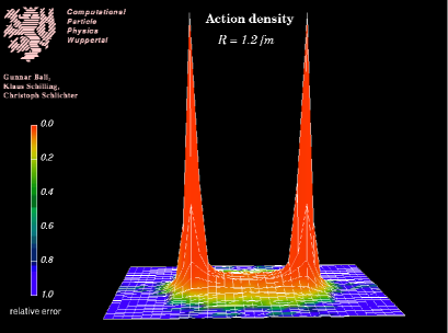
Figure 1: Lattice evidence of the interquark flux tube. Figure provided by G. Bali, see[1, 2].

Confinement and chiral symmetry breaking are the two main facts in low-energy QCD and show up explicitly in the spectrum of quark bound states. Confinement implies that the nature of the quark dynamics has to change strongly in dependence on the scale of energy or distance associated with the interaction. Let us consider the interaction between a quark and an antiquark. At short quark-antiquark distance $r$, the interaction is dominated by the one gluon exchange (dipole configuration) and is obtained by a perturbative expansion in $\alpha_{\rm s}$. With increasing distance, the interaction becomes linear in $r$ (flux tube configuration). The formation of a flux tube of constant energy density $\sigma\simeq 1{\rm GeV}/{\rm fm}$ (the so called string tension) confining the quark and the antiquark to remain bound, is the most striking feature of confinement and is inherently nonperturbative. We have hints about this flux tube from the phenomenological spectrum and the Regge trajectories. Phenomenological potential models include interactions rising with the quark-antiquark distance. Dual models explain this feature as a chromoelectric flux tube formation due to a dual Meissner effect, the QCD vacuum behaving like a t’Hooft-Mandelstam superconductor. Confinement is then due to monopoles condensation.

Lattice studies of the electric and magnetic fields strength distributions around a static quark-antiquark pair yield direct evidence and a detailed picture of the string formation (see Fig.1). Lattice data provide us with: a quark-antiquark static potential linear for $r>0.2\,{\rm fm}$; an interquark flux tube structure with a transversal rms width ranging between $0.5\,{\rm fm}$ and $0.75\,{\rm fm}$; positive tests of monopole condensations; Abelian projected electric fields and currents distributions in agreement with the dual Ginzburg Landau predictions[2, 3].

The lattice remains the most suitable tool to obtain nonperturbative information. However, most of these appear as independent and uncorrelated measurements. On the other side we have many phenomenological models implementing confinement. Finally, high order perturbative calculations are also available. In order to gain some insight in the mechanism of confinement and flux tube formation we need a model-independent, exact (in the sense that it contains perturbative and nonperturbative physics and is valid at any scale), gauge-invariant and systematic approach to the quark interaction. It helps to have a formulation which is closely related to the lattice, allows analytic calculations and is physically transparent.

In Secs. 2 and 3 we show that this program is realizable in the heavy quark case since a small expansion parameter (the quark velocity $v$) still exists. The result obtained is model independent and suitable for lattice evaluation. An analytic evaluation is possible once a QCD vacuum model is considered. Therefore it is possible to test models of confinement in an unambiguous and direct relation with the phenomenological and lattice data.

We know that in the low energy region new degrees of freedom become relevant. The flux tube formation hints to the fact that dynamical gluon effects are vital when attempting to incorporate nonperturbative interaction, indeed the gluonic degrees of freedom are condensed into stringlike flux tube. Hence, the flux tube should determine the nonperturbative bound state quark dynamics. On one side, this means that also excited states of the interquark string has to be considered. This leads to the consideration of hybrids states and was discussed by Michael[4] at this Conference. On the other side, this means that even when considering the ground state of the interquark glue, the flux tube energy should be taken into account properly. Moreover, to understand the transition region, we should be able to control precisely how the collective behavior of gluons modifies and alters single gluon exchange.

In Secs. 4, 5 and 6 we discuss the heavy quark dynamics in QCD vacuum models that reproduce the flux tube structure, in comparison with the lattice data and with the “${1/Q^{4}}$” models extensively used in the literature. We find that all the ’flux tube models’ predict the same form for the heavy quark interaction also in the intermediate region. We show that the Gaussian dominance of the Wilson loop average has to be related with the Abelian dominance of infrared QCD establishing a connection with the dual superconductor mechanism.

In Secs. 7 and 8 we extend our discussion to bound systems involving at least one light quark. Here the spontaneous chiral symmetry symmetry breaking emerges in an interplay with confinement.

2 Gauge-Invariant approach to quark bound states

We consider a gauge invariant quark-antiquark singlet state

$$|\phi_{\alpha\beta}^{lj}\rangle\equiv{\delta_{lj}\over\sqrt{3}}\bar{\psi}^{i}_{\alpha}(x)U^{ik}(x,y,C)\psi^{k}_{\beta}(y)|0\rangle$$ (1)

where $i,j,k,l=1,\dots 3$ are color indices and the Schwinger string line $U$ has been inserted to ensure gauge-invariance

$$U(x,y;C)=P\exp\{ig\int_{y,C}^{x}A_{\mu}(z)dz^{\mu}\}.$$ (2)

At a time $t=0$, a quark and an antiquark are created, interact while propagating for a time time $t=T$ at which they are annihilated. Then, the quark-antiquark interaction is contained in the gauge-invariant four-point Green function ($x_{j}=({\bf x}_{j},T)$, $y_{j}=({\bf y}_{j},0)$)

$$\!\!\!\!\!\!\!G(x_{1},x_{2},y_{1},y_{2})={1\over Z}\int{\cal D}A\,TrS(x_{2},y_{2};A)U(y_{2},y_{1})S(y_{1},x_{1};A)U(x_{1},x_{2})e^{iS_{\rm YM}}$$ (3)

where we neglected the fermionic determinant and the annihilation terms, $Tr$ is the color trace and $S(y,x;A)$ is the quark propagator in the external field $A$. To find a closed expression for the Green function in Eq.(3) is quite a formidable task. However, the situation becomes simpler if we consider the case of heavy quarks. In the static limit $m\to\infty$ the equation for the static quark propagator

$$(i\gamma_{0}D_{0}-m)S_{0}(x,y;A)=\delta^{4}(x-y)$$ (4)

is solvable in closed form [6, 7] and we find [8, 6, 9]

$$G(T){\buildrel m_{j}\to\infty\over{\longrightarrow}}\delta^{3}({\bf x}_{1}-{\bf y}_{1})\delta^{3}({\bf x}_{2}-{\bf y}_{2})e^{-i(m_{1}+m_{2})T}\langle W(\Gamma_{0})\rangle$$ (5)

where

$$\langle W(\Gamma_{0})\rangle={1\over Z}\int{\cal D}A\,TrP\exp\big{\{}{ig\oint_{\Gamma_{0}}dz^{\mu}A_{\mu}(z)}\big{\}}\exp\{igS_{\rm YM}\big{\}}$$ (6)

is the static Wilson loop average, the loop $\Gamma_{0}$ being a rectangle. From the Feynman–Kac formula and Eq. (5) we get

$$V_{0}(r)=\lim_{T\to\infty}{i\over T}\ln\langle W(\Gamma_{0})\rangle.$$ (7)

The static quark-antiquark potential, if exists, is given in terms of the static Wilson loop average. Notice that this is an exact expression that contains both the perturbative and the nonperturbative dynamics. Indeed, no expansion in the coupling constant has been performed. Here and in the following sections we implicitly assume the existence of the potential and we postpone this issue to Sec 6. The spin-dependent ${1/m^{2}}$ corrections to the potential were calculated in [7, 10] considering the first correction to Eq. (4) and evaluating it on the zero order exact solution. The result is given in terms of vacuum expectation value of (color) electric and magnetic field insertions in the static Wilson loop and controls the fine and hyperfine separation in quarkonia.

However there were some residual difficulties:

• The kinetic energy terms was not considered lacking in consistency with the virial theorem.

• The spin-dependent potentials appeared as an expansion in ${1/m^{2}}$ completely missing the terms in $\ln m$ obtained at one loop in the $S$ matrix perturbative calculation of the interaction[11].

• The calculation of the nonperturbative contributions was based on several assumptions and there was no clear and unambiguous procedure to calculate the nonperturbative behavior of the v.e.v. of the field strength insertions in the static Wilson loop.

• It was not clear when a potential description was holding.

The solution is to disentangle the different scales of the bound system ($m$, $p=mv$, $E=mv^{2}$, $v$ being the heavy quark velocity) and to establish a systematic , unambiguous and exact expansion procedure. This will be reported in the next section.

3 Analytic closed expression for the heavy quark interaction

In the heavy quark systems, the existence of an expansion parameter (the inverse of the mass $m$ in the Lagrangian and the velocity $v$ of the quark as a dynamical defined power counting parameter) makes possible to establish a systematic expansion procedure. The tool is provided by NRQCD [12]. This is an effective theory equivalent to QCD and obtained from QCD by integrating out the hard energy scale $m$. The Lagrangian comes from the original QCD Lagrangian via a Foldy–Wouthuysen transformation. The ultraviolet regime of QCD (at energy scale $m$) is perturbatively encoded order by order in the coupling constant $\alpha_{\rm s}$ in the matching coefficients which appear in front of the new operators of the effective theory. This ensures the equivalence between the effective theory and the original one at a given order in $1/m$ and $\alpha_{\rm s}$. At order $1/m^{2}$ the NRQCD Lagrangian describing a bound state between a quark of mass $m_{1}$ and an antiquark of mass $m_{2}$ is [13, 14]

$$L=\psi_{1}^{\dagger}\!\left(\!iD_{0}+c^{(1)}_{2}{{\bf D}^{2}\over 2m_{1}}+c^{(1)}_{4}{{\bf D}^{4}\over 8m_{1}^{3}}+c^{(1)}_{F}g{{\bf\sigma}\cdot{\bf B}\over 2m_{1}}\right.c^{(1)}_{D}g{{\bf D}\!\cdot\!{\bf E}-{\bf E}\!\cdot\!{\bf D}\over 8m_{1}^{2}}$$

$$+\left.ic^{(1)}_{S}g{{\bf\sigma}\!\!\cdot\!\!({\bf D}\!\times\!{\bf E}-{\bf E}\!\times\!{\bf D})\over 8m_{1}^{2}}\!\right)\psi_{1}+\hbox{\, antiquark terms}\,(1\leftrightarrow 2)+{d_{1}\over m_{1}m_{2}}\psi_{1}^{\dagger}\psi_{2}\psi_{2}^{\dagger}\psi_{1}$$

$$+{d_{2}\over m_{1}m_{2}}\psi_{1}^{\dagger}{\bf\sigma}\psi_{2}\psi_{2}^{\dagger}{\bf\sigma}\psi_{1}+{d_{3}\over m_{1}m_{2}}\psi_{1}^{\dagger}T^{a}\psi_{2}Q_{2}^{\dagger}T^{a}\psi_{1}+{d_{4}\over m_{1}m_{2}}\psi_{1}^{\dagger}T^{a}{\bf\sigma}\psi_{2}\psi_{2}^{\dagger}T^{a}{\bf\sigma}\psi_{1}.$$ (8)

This is the relevant Lagrangian in order to calculate the bound state energies up to order $O(v^{4})$. The coefficients $c^{(j)}_{2}$, $c^{(j)}_{4}$, … are evaluated at a matching scale $\mu$ for a particle of mass $m_{j}$. The matching coefficients are $1$ or $0$ at the tree level. At one loop they contain terms in $\ln m_{j}$ which establish [15] the agreement of the present calculation with the result for the perturbative interaction obtained at one loop in the $S$ matrix formalism[11]. For simplicity in the following we consider the tree level values .

With Eq. (8) we have reduced the heavy quark dynamics to a nonrelativistic Schrödinger theory for the heavy quark (antiquark) with Pauli propagator $K$ coupled to the usual relativistic field theory for light quark (omitted here, quenched appr.) and gluons. This result is especially useful for calculation on coarse lattice [12]. However, here we are looking for analytic results. The strategy is the following [16, 17]. At the $O(v^{2})$ the Pauli propagator satisfies the equation

$$i\frac{\partial}{\partial x^{0}}K_{j}=\left[m_{j}+\frac{1}{2m_{j}}({\bf p}_{j}-g{\bf A})^{2}\right.-\frac{1}{8m_{j}^{3}}({\bf p}_{j}-g{\bf A})^{4}+gA^{0}$$ (9)

$$\ -\frac{g}{m_{j}}{\bf S}_{j}\cdot{\bf B}-\frac{g}{8m_{j}^{2}}(\partial_{i}E^{i}-ig[A^{i},E^{i}])\left.+\frac{g}{4m_{j}^{2}}\varepsilon^{ihk}S_{j}^{k}\{(p_{j}-gA)^{i},E^{h}\}\right]K_{j}$$

and therefore admits a path integral representation

$$K_{j}(x,y|A)=\int{\cal D}[{\bf z}_{j},{\bf p}_{j}]\,{\rm T}_{s}\,e^{i\int dt\,[{\bf p}_{j}\cdot\dot{{\bf z}}_{j}-H]}$$ (10)

where $H$ is the Hamiltonian appearing in (9). Starting, as in Sec. 2, from the $q\bar{q}$ Green function (3), we can substitute the quark Dirac propagator with the Pauli propagator and use Eq. (10) to obtain the closed path integral representation

$$\!\!\!\!\!\!\!\!\!\!\!\!\!\!\!\ G(T)\longrightarrow K(T)=\int{\cal D}[{\bf z}_{1},{\bf p}_{1}]\int{\cal D}[{\bf z}_{2},{\bf p}_{2}]\exp\left\{i\!\int\!dt\,\sum\left[{\bf p}_{j}\cdot\dot{{\bf z}}_{j}-m_{j}-\frac{{\bf p}^{2}_{j}}{2m_{j}}+\frac{{\bf p}^{4}_{j}}{8m_{j}^{3}}\right]\right\}$$

$$\times\,\left\langle\frac{1}{3}{\rm Tr\,T_{s}\,P}\exp\left\{ig\oint_{\Gamma}dz^{\mu}\,A_{\mu}(z)\right.\right.+$$ (11)

$$\sum_{j=1}^{2}\frac{ig}{m_{j}}\int_{\Gamma_{j}}dz^{\mu}\big{(}S_{j}^{l}\hat{F}_{l{\mu}}(z)-\frac{1}{2m_{j}}S_{j}^{l}\varepsilon^{lkr}p_{j}^{k}F_{{\mu}r}(z)\left.\left.-\frac{1}{8m_{j}}D^{\nu}F_{{\nu}{\mu}}(z)\big{)}\right\}\right\rangle$$

with $\langle f[A]\rangle\equiv{1\over Z}\int{\cal D}A\,f[A]\exp\{iS_{\rm YM}\}$ , $T_{\rm s}$ spin ordering and $P$ path ordering. Notice that now the kinetic energy of the quark is explicitly considered and the contour integral in $A_{\mu}$ and $F_{\mu\nu}$ is extended to the distorted Wilson loop in Fig. 2. Indeed, due to the presence of the path integral sum, we are considering any possible trajectory for the quark (antiquark) at variance with the static path of the previous section.

b

Figure 2: Distorted Wilson loop.

Then, the potential exists if we can make the following identification in (11)

$$\left\langle\frac{1}{3}{\rm Tr}\cdots\right\rangle={\rm T_{s}}\exp\left[-i\int dt\,V({\bf z},{\bf p},{\bf S})\right].$$ (12)

From Eqs.(11) and (12) we find [16]

$$\int_{t_{\rm i}}^{t_{\rm f}}dtV_{{\rm Q}\bar{{\rm Q}}}=i\log\langle W(\Gamma)\rangle$$ (13)

$$-\sum_{j=1}^{2}\frac{g}{m_{j}}\int_{{\Gamma}_{j}}dz^{\mu}\left.\Big{(}S_{j}^{l}\,\langle\!\langle\hat{F}_{l\mu}(z)\rangle\!\rangle\right.-\frac{1}{2m_{j}}S_{j}^{l}\varepsilon^{lkr}p_{j}^{k}\,\langle\!\langle F_{\mu r}(z)\rangle\!\rangle-\left.\frac{1}{8m_{j}}\,\langle\!\langle D^{\nu}F_{\nu\mu}(z)\rangle\!\rangle\right.\Big{)}$$

$$-\sum_{j,j^{\prime}=1}^{2}\frac{ig^{2}}{2m_{j}m_{j^{\prime}}}{\rm T_{s}}\int_{{\Gamma}_{j}}dz^{\mu}\,\int_{{\Gamma}_{j^{\prime}}}dz^{\prime\sigma}\,S_{j}^{l}\,S_{j^{\prime}}^{k}\left(\,\langle\!\langle\hat{F}_{l\mu}(z)\hat{F}_{k\sigma}(z^{\prime})\rangle\!\rangle-\right.\left.\langle\!\langle\hat{F}_{l\mu}(x)\rangle\!\rangle\,\langle\!\langle\hat{F}_{k\sigma}(x^{\prime})\rangle\!\rangle\right)$$

where $\langle\!\langle f(A)\rangle\!\rangle\equiv\langle f(A)W(\Gamma)\rangle/\langle W(\Gamma)\rangle$ is the vacuum expectation value in presence of a quark–antiquark pair (i.e. the Wilson loop). Eq. (13) is the quark-antiquark potential at order $v^{2}$ of the systematic expansion in $v$. No expansion in the coupling constant has been performed. The result is physically transparent. In Eq. (13) the first term contains the static and the velocity-dependent potential, the second is the magnetic interaction, the third is the Thomas precession, the fourth is the Darwin term and the last one is the spin-spin interaction. All the dynamics is contained in the Wilson loop and in the v.e.v. of field strength in presence of the Wilson loop, hence is pure gluodynamics. Had we worked in QED, we would obtain the same result as in (13). Notice that the coupling underlying (13) is the vectorial coupling of the Dirac equation. The difference between QED and QCD is contained in the behavior of the v.e.v. of field strengths and Wilson loop. The non linear dynamics of QCD determines the nonperturbative behavior of these v.e.v and accounts for the difference with QED.

Varying the quark path $z_{j}^{\mu}(t)\rightarrow z_{j}^{\mu}(t)+\delta z_{j}^{\mu}(t)$, the Mandelstam formula can be obtained

$$\ g\langle\!\langle F_{\mu\nu}(z_{j})\rangle\!\rangle=(-1)^{j+1}{\delta i\log\langle W(\Gamma)\rangle\over\delta S^{\mu\nu}(z_{j})}$$

$$\ g^{2}\!\left(\!\langle\!\langle F_{\mu\nu}(z_{1})F_{\lambda\rho}(z_{2})\rangle\!\rangle-\langle\!\langle F_{\mu\nu}(z_{1})\rangle\!\rangle\langle\!\langle F_{\lambda\rho}(z_{2})\rangle\!\rangle\!\right)=-ig{\delta\over\delta S^{\lambda\rho}(z_{2})}\langle\!\langle F_{\mu\nu}(z_{1})\rangle\!\rangle$$

with $\delta S^{\mu\nu}(z_{j})=dz_{j}^{\mu}\delta z_{j}^{\nu}-dz_{j}^{\nu}\delta z_{j}^{\mu}$. We conclude that to obtain the complete quark-antiquark order $O(v^{2})$ interaction (quenched) no other assumptions are needed than the behavior of $\langle W(\Gamma)\rangle$: given $\langle W(\Gamma)\rangle$ everything is analytically calculable. On the other side, expanding the average on the distorted Wilson loop $\Gamma$ in terms of the static Wilson loop $\Gamma_{0}$ we get expressions for the potentials suitable for lattice evaluation [18]. Then, the way to validation of analytic models of the QCD vacuum via lattice data and phenomenological data is open. The aim is to obtain information as much as possible model-independent on the nonperturbative dynamics.

3.1 General form of the potential

At the order $O(v^{2})$ and with tree level matching coefficients the quark-antiquark interaction reads

$$V=V_{0}+V_{\rm SD}+V_{\rm VD}$$ (14)

with the spin-dependent interaction

$$\!\!\!\!\!\!\!\!\!V_{\rm SD}={1\over 8}\left({1\over m_{1}^{2}}+{1\over m_{2}^{2}}\right)+\Delta\left[V_{0}(r)+V_{\rm a}(r)\right]\left({{\bf L}_{1}\cdot{\bf S}_{1}\over 2m_{1}^{2}}-{{\bf L}_{2}\cdot{\bf S}_{2}\over 2m_{2}^{2}}\right){1\over r}\left[V^{\prime}_{0}(r)+2V^{\prime}_{1}(r)\right]$$ (15)

$$\!\!\!\!\!\!\!\!+{1\over m_{1}m_{2}}\left({\bf L}_{1}\cdot{\bf S}_{2}-{\bf L}_{2}\cdot{\bf S}_{1}\right){V^{\prime}_{2}(r)\over r}+{1\over m_{1}m_{2}}\left({{\bf S}_{1}\cdot{\bf r}\>{\bf S}_{2}\cdot{\bf r}\over r^{2}}-{{\bf S}_{1}\cdot{\bf S}_{2}\over 3}\right)V_{3}(r)+{{\bf S}_{1}\cdot{\bf S}_{2}\over 3m_{1}m_{2}}V_{4}(r)$$

where ${\bf L}_{j}={\bf r}\times{\bf p}_{j}$, and the velocity-dependent interaction is given by ($\Big{\{}~{}~{}\Big{\}}=$ Weyl ordering),

$$V_{\rm VD}={1\over m_{1}m_{2}}\left\{{\bf p}_{1}\cdot{\bf p}_{2}V_{\rm b}(r)\right\}+{1\over m_{1}m_{2}}\left\{\left({{\bf p}_{1}\cdot{\bf p}_{2}\over 3}-{{\bf p}_{1}\cdot{\bf r}~{}{\bf p}_{2}\cdot{\bf r}\over r^{2}}\right)V_{\rm c}(r)\right\}$$

$$+\sum{1\over m_{j}^{2}}\left\{p^{2}_{j}V_{\rm d}(r)\right\}+\sum{1\over m_{j}^{2}}\left\{\left({p^{2}_{j}\over 3}-{{\bf p}_{j}\cdot{\bf r}~{}{\bf p}_{j}\cdot{\bf r}\over r^{2}}\right)V_{\rm e}(r)\right\}.$$ (16)

The dynamics is contained in the $V_{i}(r)$ functions. These can be evaluated analytically via functional derivatives or expansion of the Wilson loop (once its nonperturbative behavior is assigned in a vacuum model), see [19, 16] or can be evaluated numerically on the lattice from v.e.v. of field strength insertions in the static Wilson loop, see[18, 20]. The spin-dependent potentials agree with the Eichten-Feinberg result [7]. The velocity dependent potentials were obtained in [16, 18] and have to be taken into account to be consistent at the order $v^{2}$ of the systematic expansion. The lattice results are presented in Sec. 5 while in the next Section we summarize the analytic results obtained in various models of the QCD vacuum. The common thread of these models is reproducing the interquark flux tube structure.

4 Infrared dynamics and flux tube structure

The expression (13) for the heavy quark interaction is exact at the order of the expansion in $v$ considered. It is gauge-invariant and this allows us to insert approximations, i.e. vacuum models to get the nonperturbative behavior of the Wilson loop average. We retain the relevant configuration in the nonperturbative regime, which turns out to be a flux-tube like configuration.

4.1 A simple model calculation

The simplest model consist in assuming that the short and the long range contributions to the Wilson loop factorize and evaluating the last one using an area law (as suggested by the strong coupling expansion)

$$\log\langle W(\Gamma)\rangle=\log\big{[}\langle W(\Gamma)\rangle^{\rm SR}\cdot\langle W(\Gamma)\rangle^{\rm LR}\big{]}=-\frac{4}{3}g^{2}\oint_{\Gamma}dx^{\mu}\oint_{\Gamma}dy^{\nu}D_{\mu\nu}(x-y)+\sigma S_{\rm min}+{C\over 2}{\cal P}.$$ (17)

$D_{\mu\nu}$ is the free gluon propagator, $\sigma$ is the string tension, $S_{\rm min}$ is the minimal area enclosed in the distorted Wilson loop contour (cf. Fig. 2), $C$ is a constant and ${\cal P}$ is the perimeter of the loop. The general expression for the minimal surface with contour $\Gamma$ is the Nambu-Goto action. In ref.[16], it is shown that, at the order $v^{2}$ of the interaction, the minimal area is equivalent to the area spanned by straight lines connecting points at equal time on the quark and antiquark trajectories. For any details we refer to [16, 19]. Here, we only present the final result of this minimal area law model (MAL)

$$\!\!\!\!\!\!\!\!\!\!\!\!\!V_{0}(r)=-{4\alpha_{\rm s}\over 3r}+\sigma r+C\,\,\,V_{\rm b}(r)={8\alpha_{\rm s}\over 9r}-{\sigma\over 9}r\,\,\,V_{\rm c}(r)=-{2\alpha_{\rm s}\over 3r}-{\sigma\over 6}r\quad V_{\rm d}(r)=-{\sigma\over 9}r-{C\over 4}$$

$$\!\!\!\!\!\!\!\!\!\!\!\!V_{\rm e}(r)=-{\sigma\over 6}r\quad V^{\prime}_{1}(r)=-\sigma\quad V^{\prime}_{2}(r)={4\alpha_{\rm s}\over 3r^{2}}\quad V_{3}(r)=4{\alpha_{\rm s}\over r^{3}}\quad V_{4}(r)={32\over 3}\pi\alpha_{\rm s}\delta^{3}({\bf r})$$ (18)

and $\Delta V_{\rm a}=0$. The one gluon exchange term (proportional to $\alpha_{\rm s}$) coincides with the usual Breit-Fermi potential. Let us focus on the nonperturbative part (in $\sigma$ and $C$). The $V_{1}-V_{4}$ spin potentials (sd) agree with the electric confinement calculation of Eichten and Feinberg[7] (taking into account the Gromes correction[10]). The $V_{\rm a}-V_{\rm e}$ velocity potentials (vd) were first calculated in MAL[16, 18]. To make clear the physical content of the result, let us write the nonperturbative contributions in the center of mass system for equal masses. The spin-dependent part is

$$V_{\rm SD}^{NP}=-{\sigma\over 2m^{2}r}{\bf L}\cdot{\bf S}$$ (19)

and corresponds to pure Thomas precession, i.e. the magnetic contribution is zero. The velocity dependent part is

$$V_{\rm VD}^{NP}=-{\sigma\over 6}{{\bf L^{2}}\over m^{2}r}$$ (20)

and it is proportional to the flux tube angular momentum. Indeed, the same vd correction is obtained in the relativistic flux tube model [21] where the energy of the interquark flux tube is explicitly added to the Hamiltonian. Then, it is clear that our gauge-invariant Wilson loop approach has automatically included the energy of the flux tube.

The result is even more interesting since it cannot be obtained within the semirelativistic reduction of a pure convolution (i.e. depending only on the momentum transfer $Q=p_{1}-p_{1}^{\prime}$) Bethe-Salpeter kernel, with any mixture of vector and scalar components. In general, a scalar ${1/Q^{4}}$ BS kernel is used in order to reproduce (19), however the velocity dependent correction differ from (20), see Sec. 5. On the other hand, the result (19)-(20) is physically transparent. Imagine a quark-antiquark pair connected by a chromoelectric flux tube. The magnetic field is zero in the comoving frame and then the spin-interaction is purely Thomas precession; the electric tube is moving with a transversal velocity and then its energy originates the vd term. This is the Buchmüller picture. We emphasize that the ’scalar-like’ character of the spin splitting we obtained is dynamically generated through the collective nature of the gluonic degrees of freedom. It is interesting that in [22] this same conclusion has been obtained working in the framework of the Coulomb gauge Hamiltonian and diagonalizing a sector of the Fock space. Again, the scalar interaction is effectively generated. However, the Wilson loop approach appears to be simpler and more powerful (at least for heavy quarks); the intermediates states that are explicitly considered in the Fock Hamiltonian approach here are summed up into the functional formalism. Expressing the potential in terms of the Wilson loop we keep the relevant degrees of freedom. Our special ’trial function’ constructed with the string interquark operator has selected out the flux tube configuration.

The MAL model is in many respects too rough (e.g. the $\langle\langle F_{\mu\nu}F_{\rho\sigma}\rangle\rangle$ v.e.v. turns out to be zero and the flux tube turns out to be infinitely thin) and it may play some role only in the limit of very large interquark distances where an effective relativistic string model description is expected to hold. In the next Sections we discuss more sophisticated assumptions.

4.2 Gaussian dominance in gluodynamics versus Abelian dominance in infrared QCD

We need models of the QCD vacuum which provide us with the nonperturbative behavior of the Wilson loop average. To this aim we want to exploit all the available lattice information on the mechanism of confinement and the measurements of Wilson loop and field strength v.e. v.. About the mechanism of confinement, at this Conference, evidence [3, 2] was presented that the QCD infrared dynamics is well approximated by a (dual) Abelian Higgs model. Indeed, in the Abelian projection the QCD gluodynamics is reduced to Abelian fields, Abelian monopoles and charged matter fields degrees of freedom. Lattice simulations show Abelian dominance and monopole dominance in the long range features of QCD and condensation of monopoles in the confined phase. For details we refer to [3, 2]. The measured electric fields and magnetic currents in the presence of static quark sources are consistent with dual Ginzburg–Landau type of equations. The penetration length $\lambda={1/M}$ ($M=$ dual gluon mass) and the correlation length $\xi={1/M_{\phi}}$ ($M_{\phi}=$ Higgs mass) are measured. It is found $M\simeq M_{\phi}$ and therefore the QCD vacuum behaves as a dual superconductor on the border between type I and type II. Flux tube solutions (of the type of Abrikosov-Nielsen-Olesen vortices) exist and the structure of these solutions is controlled by the penetration and the correlation length. However these are lattice measurements and it is not clear e.g. the relation of $\lambda$ and $\xi$ with the parameters of QCD.

On the other side, let us consider the v.e.v. of the Wilson loop. It pays to expand this average in terms of fields strength expectation values, by using the non-Abelian Stokes theorem[23]

$$\!\!\!\!\!\!\!\!\!\langle W(\Gamma)\rangle\equiv\langle\exp\{ig\oint_{\Gamma}dz_{\mu}A_{\mu}(z)\}\rangle=\langle P\exp ig\int_{S(\Gamma)}dS_{\mu\nu}(1)U(0,1)F_{\mu\nu}(1)U(1,0)\rangle=$$ (21)

$$\!\!\!\!\!\!\!\!\!\!\!\exp\{\sum_{n=0}^{\infty}{(ig)^{n}\over n!}\int_{S(\Gamma)}dS_{\mu_{1}\nu_{1}}(1)\cdots dS_{\mu_{n}\nu_{n}}(n)\langle U(0,1)F_{\mu_{1}\nu_{1}}(1)U(1,0)\cdots F_{\mu_{n}\nu_{n}}(n)U(n,0)\rangle_{\rm cum}\}$$

where $i\equiv x_{i}$, $S(\Gamma)$ denotes a surface with contour $\Gamma$ and $\langle\dots\rangle_{\rm cum}$ stands for the cumulant average[23]. In principle, the v.e.v. of the Wilson loop is given by the sum of all the cumulants. However, in a recent lattice investigation [24], evidence of the Gaussian dominance in the cumulant expansion of quasi-static Wilson loop average was found. Therefore, it follows that

$$\langle W(\Gamma)\rangle\simeq\exp\{{-{1\over 2}}\int_{S(\Gamma)}dS_{\mu\nu}(0)\int_{S(\Gamma)}dS_{\rho\sigma}(x)\langle g^{2}U(0,x)F_{\mu\nu}(x)U(x,0)F_{\rho\sigma}(0)\rangle\}$$ (22)

is a good approximation. This is the basic assumption in the (Gaussian) stochastic vacuum model [23] and it was phenomenologically confirmed by calculation in high energy scattering [25] and quarkonia. Then, the heavy quark interaction is determined by the two-point field strength correlator

$$g^{2}\langle U(0,x)F_{\mu\nu}(x)U(x,0)F_{\lambda\rho}(0)\rangle=\ {g^{2}\langle F^{2}(0)\rangle\over 24N_{c}}\bigg{\{}(\delta_{\mu\lambda}\delta_{\nu\rho}-\delta_{\mu\rho}\delta_{\nu\lambda})(D(x^{2})+D_{1}(x^{2}))$$

$$+(x_{\mu}x_{\lambda}\delta_{\nu\rho}-x_{\mu}x_{\rho}\delta_{\nu\lambda}+x_{\nu}x_{\rho}\delta_{\mu\lambda}-x_{\nu}x_{\lambda}\delta_{\mu\rho}){d\over dx^{2}}D_{1}(x^{2})\bigg{\}}.$$ (23)

In (23) the Lorentz decomposition is general and the dynamics is contained in the form factors $D$ and $D_{1}$. The function $D$ is responsible for area law and confinement (indeed in QED, due to the Bianchi identity, we have $D=0$). For $D$ and $D_{1}$ the lattice calculations[24, 26] gives an exponential long-range decreasing behavior $\simeq G_{2}\exp\{-|x|/T_{g}\}$, where $G_{2}\equiv\langle\alpha_{s}F^{2}(0)\rangle/\pi$ is the gluon condensate and $T_{g}\simeq 0.2\,{\rm fm}$ is the gluon correlation length.

In ref.[27], the QCD two–point field strength correlator (23) has been related to the dual field propagator of the effective Abelian Higgs model describing infrared QCD. In this way the Gaussian dominance in the Wilson loop average is understood as following from the classical approximation in the dual theory. Moreover, it is possible to relate the QCD parameter $T_{g}$ and $G_{2}$ to the dual parameters. In the London limit $T_{g}$ is identified with the dual gluon mass $M$, without the London limit the relation is more involved but still $T_{g}$ is expressed in terms of the dual theory parameters.

The conclusion is that we need two parameters $T_{g}$ and $G_{2}$ to describe the heavy quark dynamics and indeed they are necessary to control the structure of the flux tube. Had we only one parameter, like the string tension $\sigma$, we could encode the information of a constant energy density in the flux tube. However, the whole structure is important, and also the information about the width of the flux tube has to be considered. In the limit of very large interquark distances and in particular dynamical regimes, we can store the relevant information in one parameter, the string tension.

4.3 Vacuum models for the Wilson loop

As shown above, one obtains the $O(v^{2})$ quenched quark dynamics in a given vacuum model, simply evaluating the Wilson loop in that model. In this way the phenomenological data are put in direct relation with the assumptions on the QCD vacuum. Here we consider three models: Stochastic vacuum model (SVM)[25], dual QCD (DQCD)[28] and the flux tube model of Isgur and Paton[29]. We emphasize that these are models of the QCD vacuum, valid at the confinement scale.

$\bullet$Stochastic vacuum model. The stochastic vacuum model[25] is based on the idea that the infrared part of the QCD functional integral can be approximated by a stochastic process with a converging cluster expansion and a finite correlation length $T_{g}$. This assumption is well confirmed by the lattice data. Then, the Wilson loop is given by Eqs.(22)-(23) with parameters $T_{g}$ and $G_{2}$. The behavior of $D$ and $D_{1}$ and the value of $T_{g}$ are taken from the lattice measurements, $G_{2}$ from the phenomenological data. The static potential is

$$V_{0}(r)\simeq G_{2}\int_{0}^{\infty}d\tau\int_{0}^{r}d\lambda(r-\lambda)D(\tau^{2}+\lambda^{2})$$ (24)

and the string tension $\sigma$ emerges as an integral on the $D$ function $\sigma\simeq G_{2}\int_{0}^{\infty}d\tau\int_{0}^{\infty}d\lambda$ $D(\tau^{2}+\lambda^{2})$ in the limit ${T_{g}/r}\to 0$. The field distribution between the quark and the antiquark is a flux tube[30] with $r_{MS}\simeq 1.8\,T_{g}$. Similarly the sd and vd potential are obtained. I refer to [23, 19] for the details. Here we restrict the discussion to the long range limits of the potentials in the three vacuum models, (see the final subsection).

$\bullet$Dual QCD. DQCD[28] is a concrete realization of the Mandelstam t’Hooft dual superconductor mechanism of confinement. It describes the QCD vacuum as a dual superconductor on the border between type I and II. The Wilson loop approach supplies with a simple method to connect averaged local quantities in QCD and in dual QCD (=dual gluodynamics). For large loops we assume[28, 31]

$$\langle W(\Gamma)\rangle\simeq\langle W(\Gamma)\rangle_{Dual}={\displaystyle{\int\!{\cal D}{\cal C}\,{\cal D}{\cal B}\,\exp\left[i\int dxL(G_{\mu\nu}^{\rm S})\right]}\over\displaystyle{\int\!{\cal D}{\cal C}\,{\cal D}{\cal B}\,\exp\left[i\int dxL(0)\right]}}$$ (25)

where $C_{\mu}$ are the dual potentials, $G_{\mu\nu}$ the dual field strengths, ${\cal B}_{i}$ the monopole fields, ${L}$ the effective dual Lagrangian in the presence of quarks ${L}(G_{\mu\nu}^{\rm S})=2~{}{\rm Tr}\{-{1\over 4}{\cal G}^{\mu\nu}{\cal G}_{\mu\nu}$ $+{1\over 2}({\cal D}_{\mu}{\cal B}_{i})^{2}\}-U({\cal B}_{i})$, and $U({\cal B}_{i})$ the Higgs potential. The quark sources moving around the Wilson loop are inserted via the Dirac string tensor $G_{\mu\nu}^{\rm S}(x)=g\,\epsilon_{\mu\nu\alpha\beta}\int ds\int dt\,y^{\prime\alpha}\dot{y}^{\beta}$ $\delta(x-y)$. From (25) it follows

$$g\langle\!\langle F_{\mu\nu}(z_{j})\rangle\!\rangle={2\over 3}g\,\varepsilon_{\mu\nu\rho\sigma}\langle\!\langle G^{\rho\sigma}(z_{j})\rangle\!\rangle_{Dual}$$ (26)

and it is possible to relate the averaged values of local quantities in QCD and in the dual theory. Then Eqs.(15)-(16) produce the $O(v^{2})$ interaction in the dual formalism, for details cf.[31]. We discuss only the long range limits in the final subsection. The nonperturbative parameters are the v.e.v. of the Higgs field, ${\cal B}_{0}$, and $\kappa$, the coupling constant of the Higgs potential (from these the penetration length and the correlation length can be constructed). The flux tube configurations ($\simeq$ Abrikosov-Nielsen-Olesen vortex) with finite $r_{MS}\sim{1/M}$, $M=$ mass of the dual gluon, arise[32] from the numerical solution of the classical dual Ginzburg-Landau type of equations obtained from ${L}$. It is the presence of the Higgs field which confines transversally the energy distribution in a flux tube. Again $\sigma$ comes from the integration on a function exponentially decreasing approximately with $M$.

$\bullet$Isgur-Paton flux tube model. This model is extracted from the strong coupling limit of the QCD lattice Hamiltonian. A N-body discrete string-like model Hamiltonian describes the gluonic degrees of freedom. The limit $N\to\infty$ corresponds to a localized string with an infinite number of degrees of freedom; the radius of the flux tube is proportional to ${1/N}$. For any detail we refer to the talk of Paton in these Proceedings. In a recent paper[22], the sd potential has been obtained in this model.

4.4 Potentials and flux tube structure

It is interesting to consider the potentials obtained using these different vacuum models in the limit of large interquark distance $r$.

$\bullet$SVM

$$V_{0}(r)=\sigma r+{1\over 2}c^{(1)}\sigma\,T_{g}-c\,\sigma\,T_{g},\quad{d\over dr}V_{1}(r)=-\sigma+{c\,\sigma\,T_{g}\over r}\>,\quad{d\over dr}V_{2}(r)={c\,\sigma\,T_{g}\over r}\>,$$ (27)

$V_{3}$ and $V_{4}$ fall off exponentially as $\exp\{-{r/T_{g}}\}$ and

$$\!\!\!\!\!\!\!\!\!\!\!\!\!\!V_{\rm b}(r)=-{\sigma\over 9}r-{2\over 3}{d\,\sigma\,T_{g}^{2}\over r}+{8\over 3}{e\,\sigma\,T_{g}^{3}\over r^{2}}\>,\quad\quad V_{\rm c}(r)=-{\sigma\over 6}r-{d\,\sigma\,T_{g}^{2}\over r}+{2\over 3}{e\,\sigma\,T_{g}^{3}\over r^{2}}\>,$$ (28)

$$\!\!\!\!\!\!\!\!\!\!\!\!\!\!\!V_{\rm d}(r)=-{\sigma\over 9}r+{c\over 4}\,\sigma\,T_{g}-{c^{(1)}\over 8}\sigma\,T_{g}+{d\over 3}{\sigma\,T_{g}^{2}\over r}-{2\over 9}{e\,\sigma T_{g}^{3}\over r^{2}}\,\,\,V_{\rm e}(r)=-{\sigma\over 6}r+{d\over 2}{\sigma\,T_{g}^{2}\over r}-{e\over 3}{\sigma\,T_{g}^{3}\over r^{2}}.$$

$\bullet$DQCD

$$V_{0}(r)=\sigma r-(C+C^{(1)}){\sigma\over M}\quad\quad{d\over dr}V_{1}(r)=-\sigma+C{\sigma\over M}{1\over r}\quad\quad{d\over dr}V_{2}(r)=C{\sigma\over M}{1\over r}$$ (29)

and $V_{3}$ and $V_{4}$ fall off exponentially as $\exp\{-Mr\}$.

$\bullet$I-P flux tube model

$${d\over dr}V_{1}(r)=-\sigma\quad{d\over dr}V_{2}(r)=\lim_{N\to\infty}{\sigma\over N}$$ (30)

and $V_{3}$ and $V_{4}$ are $\simeq{1/N}$. The $c,c^{(1)},d,e$, $C,C^{(1)}$ above are numerical constants known in terms of the parameters of the models. We learn that

1) The gluon correlation length $T_{g}$ in SVM has the same role as the inverse of the dual gluon mass $M$ in DQCD and $T_{g}/r$ as the inverse of the number of degrees of freedom $N$ in the I-P flux tube model. All these quantities act like a correlation length. From now on, we use $T_{g}$ to refer to any of them.

2) The MAL results are completely contained in all these models. The MAL describes the limit of large interquark distances or better the limit ${T_{g}/r}\to 0$ which is also the limit in which a potential exists, cf. Sec. 6, or the string limit. Indeed, all the corrections to the MAL are proportional to the gluon correlation length or equivalently to the width of the flux tube: the form of these corrections is the same in all these flux tube-like models (models that predict the flux tube structure).

3) The magnetic interaction is zero only in the limit $T_{g}/r\to 0$. In the intermediate distance region is different from zero as one can see from the value of $V_{2}$. Then a purely scalar effective interaction emerges only in the long range limit.

4) $T_{g}$ controls the width and the shape of the flux tube as well as the validity of the potential description. Physically it should correspond to the size of the color domain as well as the fluctuation of the color fields.

We conclude that the results for the heavy quark interaction are essentially the same for any flux-tube model of the QCD vacuum.

5 Lattice calculations, flux tube models and ${1/Q^{4}}$ models

b

Figure 3: $V_{0}$ and $V_{1}^{\prime}$ potentials from [20].

b

Figure 4: $V_{\rm b}$ and $V_{\rm c}$ potentials from [20].

b

Figure 5: $V_{\rm d}$ and $V_{\rm e}$ potentials from [20].

An entire class of confining models for the heavy quark dynamics comes from the semirelativistic reduction of a pure convolution Bethe-Salpeter kernel (see[33] and refs. therein)

$$I(Q^{2})=\gamma_{1}^{\mu}\gamma_{2}^{\nu}P_{\mu\nu}J_{v}(Q)+J_{s}(Q)$$ (31)

where $J_{v}$ contains the one gluon exchange, $P$ is a factor depending on the gauge and $J_{s}$ has an infrared behavior like ${1/{\bf Q}^{4}}$ (or ${1/Q^{4}}$, $Q$ being the momentum transfer) chosen in order to reproduce the linear behavior of the static potential. To reproduce $V_{1}^{\prime}$ then $J_{s}$ has to be scalar. These models produce:

$$\!\!\!\!\!\!\!\!\!\!\!\!\!\!V_{0}=-{4\alpha_{\rm s}\over 3r}+\sigma r+C\quad V_{\rm b}(r)={8\alpha_{\rm s}\over 9r}+0/{2\sigma\over 3}\quad V_{\rm c}(r)=-{2\alpha_{\rm s}\over 3r}-{\sigma\over 2}r/0\quad V_{\rm d}(r)=-{\sigma\over 2}r-{C\over 4}$$

$$\!\!\!\!\!\!\!\!\!\!\!\!\!\!V_{\rm e}(r)=0\quad V^{\prime}_{1}(r)=-\sigma\quad V^{\prime}_{2}(r)={4\alpha_{\rm s}\over 3r^{2}}\quad V_{3}(r)={4\alpha_{\rm s}\over r^{3}}\quad V_{4}(r)={32\over 3}\pi\alpha_{\rm s}\delta^{3}({\bf r})$$ (32)

The two results in Eq. (32) correspond respectively to the instantaneous form of the kernel ${1/{\bf Q}^{4}}$ or to the inclusion of retardation corrections as in [34]. Notice that: 1) These models are constructed in order to reproduce $V_{1}$ as given in Eq. (18). 2) They cannot reproduce the behavior of the $V_{\rm VD}^{NP}$ (20) (even adding retardation corrections or allowing a mixture of vector and scalar confining kernels[34]). 3) The ${1/Q^{4}}$ propagator does not avoid the spreading of the flux tube between the quarks even if the integrated energy increases linearly with the distance between the quarks.

We conclude that a linear confining behavior with the correct spin-orbit is not sufficient to characterize the heavy quark dynamics at the order $O(v^{2})$. On the other hand the $v^{2}$ corrections to the potential are connected to v.e.v. of field strengths insertion in the Wilson loop and therefore to the energy density and to the interquark flux tube structure. The $1/Q^{4}$ models fail to take into account the dynamical nature of the glue. In Figs. 3-5 we present the latest lattice results for the potentials[20]. The lines are the MAL predictions (18). The static potential is clearly linear for $r>0.2\,{\rm fm}$ (recent results indicate that the string breaking happens for $r>0.2\,{\rm fm}$ [2]). The nonperturbative behavior of $V_{1}^{\prime}$ is consistent with the result (18) and (32). Unfortunately, the lattice data for the vd potential are not yet sufficiently accurate to discriminate between the flux tube model and the ${1/Q^{4}}$ predictions. Notice that an accurate measurement of $V_{\rm e}$ provides a good test since it is predicted to be zero in ${1/Q^{4}}$ models.

Phenomenological applications to the bottomonium and charmonium spectrum show that the vd corrections of the type (18) do not induce the deviations from the data originated by the vd corrections (32)[35].

6 On the validity of the potential description

In the previous sections we assumed that a potential description holds. This is not always the case. We know from the Lamb-shift in QED that at some order of the perturbative expansion the ultrasoft photons start giving a contribution to the energy not of a potential type. This is certainly true also in QCD but here we cannot rely only on the perturbative calculation. Then, the situation becomes more interesting and again the flux tube configuration plays a role. We can extract a potential as far as the adiabatic approximation holds, i.e., as far as the gluon time scale is short compared to the orbital period of the quarks $T_{g}\ll T_{q}$. In this case we are describing a $q\bar{q}$ pair moving in the adiabatic potential corresponding to the ground state energy of the gluon field, i.e. the ground state flux tube. The next adiabatic surface describes an excited state of the glue: an hybrid [4]. If these adiabatic surfaces are well separated, still each of them can be described with a potential. The situation is controlled by the gluon correlation length $T_{g}$ which is proportional to the this difference. The quark dynamics is simply given in terms of the two-point correlator (23) whose nonperturbative exponential decreasing behavior is controlled by $T_{g}$. In the case in which $T_{g}$ is small with respect to the other physical scales of the problem we recover the potential description, in the opposite limit we recover the sum rules description with local condensates à la Leutwyler-Voloshin [36]. Therefore there is no discrepancy between these two descriptions. However, the $c\bar{c}$ and $b\bar{b}$ systems lie in the situation in which $T_{g}$ is small compared to the other scales. Just for the ground state of the $b\bar{b}$ both descriptions can be undertaken.

Recently a new effective theory has been obtained from NRQCD integrating out the relative momentum scale. It is called potential non relativistic QCD (pNRQCD) and was presented at this Conference by J. Soto [37]. The theory describes ultrasoft gluons and the matching coefficients are the potentials. pNRQCD could be a powerful tool to understand the relation between ultrasoft degrees of freedom and nonpotential nonperturbative glue.

7 Confinement, flux tube and chiral symmetry

As soon as the light quarks enter the game we are left without any expansion parameter to develop any well–founded calculation of the quark dynamics. Even in the simplest case, a meson formed by a light and a heavy quark, we are far away from the intuitive description developed for the heavy–heavy bound states. Indeed, in this case the heavy quark is surrounded by the fuzzy cloud of the light degrees of freedom. This picture is naively completely different from a flux tube picture. Moreover chiral symmetry breaking should appear. Here, we address the issue whether the Wilson loop formalism still helps to understand the quark dynamics. If this is the case we are in the position to study the interplay between confinement and chiral symmetry breaking.

Let us consider the simplest system, the heavy-light bound state. Heavy-light systems are understood in terms of heavy quark effective theory (HQET), but HQET cannot predict the spectrum of the ’brown muck’ since this is determined by the dynamics of strong QCD. In the limit $m_{Q}\gg\Lambda_{QCD}$, HQET organizes a systematic expansion of the physical quantities in terms of $\Lambda_{\rm QCD}/m_{Q}$ and $\alpha_{\rm s}(m_{Q})$. The meson mass is given as

$$m_{M}=m_{Q}+\bar{\Lambda}+O\left({1\over m_{Q}}\right)\,\,{\rm corrections}.$$ (33)

The parameter $\bar{\Lambda}$ can be fixed on the data but its actual calculation needs a dynamical input. In the no-recoil limit $m_{Q}\to\infty$, the usual choice is to take a scalar Dirac equation to get the $\bar{\Lambda}$ parameter as an eigenvalue. The motivation is reproducing the spin-orbit splitting and the fact that this kind of equation is mathematically well behaving. There are a number of reasons against this choice:

• It breaks explicitly chiral symmetry.

• We have shown that scalar confinement arises effectively for heavy quark interaction due to the collective nature of the nonperturbative gluonic degrees of freedom.

In the next section we address the problem in the Wilson loop formalism.

7.1 Gauge-invariant approach to heavy-light quark systems

We start from the gauge-invariant quark-antiquark Green function in the Feynman-Schwinger representation [38, 39]:

$$\!\!\!\!\!\!\!\!\!\!\!\!\!G(x,u,y,v)={1\over 4}\Bigg{\langle}{\rm Tr}\,{\rm P}\,(i\,{D\!\!\!\!/}_{y}^{\,(1)}+m_{1})\,\int_{0}^{\infty}dT_{1}\int_{x}^{y}{\cal D}z_{1}e^{\displaystyle-i\,\int_{0}^{T_{1}}dt_{1}{m^{2}+\dot{z}_{1}^{2}\over 2}}$$

$$\times\int_{0}^{\infty}dT_{2}\int_{v}^{u}{\cal D}z_{2}e^{\displaystyle-i\,\int_{0}^{T_{2}}dt_{2}{m^{2}+\dot{z}_{2}^{2}\over 2}}e^{\displaystyle ig\oint_{\Gamma}dz^{\mu}A_{\mu}(z)}$$

$$\times e^{\displaystyle i\,\int_{0}^{T_{1}}dt_{1}{g\over 4}\sigma_{\mu\nu}^{(1)}F^{\mu\nu}(z_{1})}e^{\displaystyle i\,\int_{0}^{T_{2}}dt_{2}{g\over 4}\sigma_{\mu\nu}^{(2)}F^{\mu\nu}(z_{2})}(-i\,\buildrel\leftarrow\over{D\!\!\!\!/}_{v}^{\,(2)}+m_{2})\Bigg{\rangle}.$$

Again the dynamics is contained in the Wilson loop, that now looks like Fig. 6.

b

Figure 6: The Wilson loop in the static limit of the heavy quark and the interaction kernel $K$.

We can exploit the symmetry of the situation, taking the modified coordinate gauge $A_{\mu}(x_{0},{\bf 0})=0,\,x^{j}A_{j}(x_{0},{\bf x})=0$ ($A_{0}(x)=\int_{0}^{1}d\alpha x^{k}F_{k0}(x_{0},\alpha{\bf x})$, $A_{j}(x)=\int_{0}^{1}d\alpha\alpha x^{k}F_{kj}(x_{0},\alpha{\bf x}))$ in which

$$W(\Gamma)={Tr\,}{P\,}\exp\left\{ig\int_{x}^{y}dz^{\mu}A_{\mu}(z)\right\}.$$ (35)

At this point, at variance from the heavy quark case, we have to make a model dependent assumption: we consider still valid the dominance of the bilocal correlator with a finite correlation length. Under this assumption we obtain a Dirac like equation for the light quark in presence of the heavy quark. Approximating the Wilson loop as

$$\langle W(\Gamma)\rangle = \exp\left\{-{g^{2}\over 2}\int_{x}^{y}dx^{\prime\mu}\int_{x}^{y}dy^{\prime\nu}D_{\mu\nu}(x^{\prime},y^{\prime})\right\},$$ (36)

$$D_{\mu\nu}(x,y) \equiv x^{k}y^{l}\int_{0}^{1}d\alpha\,\alpha^{n(\mu)}\int_{0}^{1}d\beta\,\beta^{n(\nu)}\langle F_{k\mu}(x^{0},\alpha{\bf x})F_{l\nu}(y^{0},-\beta{\bf y})\rangle$$

where $n(0)=0$ and $n(i)=1$, we obtain the Dirac–like equation for the light quark propagator

$$S_{D}=S_{0}+S_{0}KS_{D}$$ (37)

with a kernel $K(y^{\prime},x^{\prime})\equiv\gamma^{\nu}S_{0}(y^{\prime},x^{\prime})\gamma^{\mu}D_{\mu\nu}(x^{\prime},y^{\prime})$, given diagrammatically in Fig. 6. Notice that[38]: 1) $K$ is not a translational invariant quantity: the coordinate gauge breaks explicitly this symmetry in the propagator. Physically this is due to the presence of the heavy quark. Indeed Eq. (37) is an integral equation for the light quark propagator in the field of the heavy quark. 2) The kernel depends on $D_{\mu\nu}$ which in turns is given in terms of the two-point correlator (23). Then, the heavy-light dynamics is controlled by the same two parameters controlling the heavy-heavy dynamics, $T_{g}$ and $G_{2}$. 3) The problem has many relevant scales: the light mass $m$, the correlation length $T_{g}\sim\Lambda_{QCD}$, the characteristic energy and momentum of the bound states. We have different dynamical regimes in dependences on the relative values of these scales. Let us study the various situations. In the following we consider only the nonperturbative dynamics[38].

• Potential Case: $m>{1/T_{g}}>p_{0}-m,{\bf p},{\bf p}-{\bf q}$. We neglect the negative energy states and expand the kernel $K$ in $m$. We obtain:

  $$\!\!\!\!\!\!\!\!\!\!\!\!V(r)\sim G_{2}\big{\{}\int_{-\infty}^{+\infty}d\tau\int_{0}^{r}d\lambda(r-\lambda)D(\tau^{2}+\lambda^{2})+{{\bf\sigma}\cdot{\bf L}\over 4m^{2}r}\int_{-\infty}^{+\infty}d\tau\int_{0}^{r}d\lambda\left({2\lambda\over r}-1\right)D(\tau^{2}+\lambda^{2})\big{\}}$$ (38)

  which coincides in the limit of large $r$ with the Eichten-Feinberg potential (18) with $\sigma$ as defined in the SVM section. We emphasize that the Lorentz structure which gives origin to the negative sign in front of the spin-orbit potential (hence to the Thomas precession term) is in our case not simply a scalar ($K\simeq\sigma\,r$).

• Sum Rules case: $({1/T_{g}}<p_{0}-m$, ${1/T_{g}}<m)$. We get the well-known Shifman, Vainshtein and Zakharov result for the heavy quark condensate

  $$\langle\bar{Q}Q\rangle=-\int{d^{4}p\over(2\pi)^{4}}\int{d^{4}q\over(2\pi)^{4}}{\rm Tr}\left\{S_{0}(q)K(q,p)S_{0}(p)\right\}=-{1\over 12}{\langle\alpha F^{2}(0)\rangle\over\pi m}.$$

• $D_{s}$ and $B_{s}$ case: ${1/T_{g}}>m$. For $D_{s}$ and $B_{s}$ one can still assume that the propagator inside the kernel is free and solve the equation to get the spectrum.

• $D$ and $B$ case: $m\ll{1/T_{g}}$. The nonlinear equation[40, 41]

  $$S_{D}=S_{0}+S_{0}K(S_{D})S_{D}$$ (39)

  has to be solved with Schwinger–Dyson like techniques. Notice that in the limit $m\to 0$ the form of the kernel $K$ is such that the interaction turns out to be chiral symmetric. In Ref.[41] a solution of the gap equation corresponding to Eq. (39) (with a simplified form of the interaction) was found. In that case it was possible to disentangle the translational invariant part of the interaction (the self-energy) from the non-invariant part (the bound state interaction). In this way one obtains the light quark condensate

  $$\langle 0|\bar{q}q|0\rangle\sim-T_{g}G_{2}$$ (40)

  and the heavy-light bound state energy spectrum. The result (40) looks appealing: it establishes a connection between the gluon condensate and the light quark condensate. The connection is possible since the non-local gluon condensate has introduced into the game a finite correlation length $T_{g}$. The same quantity that controls the width of the flux tube as well as the validity of the potential description in the case of heavy quarks.

In conclusion we have reached some insight in the interplay between confinement and chiral symmetry breaking, obtaining for the first time an unified framework for sum rules, potential models and chiral symmetry breaking studies.

8 Gauge-invariant approach to light-light quark systems

The starting point is again Eq. (7.1). The dynamics is contained in the distorted Wilson loop of Fig. 2. In this situation it does not exist a choice of the gauge like the modified coordinate gauge in the heavy-light case, i.e. it is not possible to get rid of both the final Schwinger strings. A result for the nonperturbative BS kernel can still be obtained in the form of effective diagrams[39] but gauge-invariance is lost. Even recovering the potential from such a kernel appears to be problematic.

9 Conclusions

We have shown that the $O(v^{2})$ heavy quark interaction is controlled only by the Wilson loop behavior: heavy quarks are a nice laboratory to test QCD vacuum models with respect to lattice and phenomenological data. On the other hand, the Wilson loop is a good approach to the quark dynamics: it keeps automatically the relevant degrees of freedom and includes naturally the flux tube configurations. The description of the heavy quark interaction needs two nonperturbative parameters $T_{g}$ and $G_{2}$: these give origin to $\sigma$ only in particular dynamic situations. $T_{g}$ controls the width and the shape of the flux tube, as well as the validity of the potential description. Any model of the QCD vacuum reproducing the interquark flux tube structure gives the same prediction for the nonperturbative heavy quark interaction. On the other hand, the class of ${1/Q^{4}}$ models give definite different predictions.

Moreover, the Wilson loop formalism appears to be useful in selecting the relevant configurations also in situations where an intuitive flux tube picture does not exist: e.g. the heavy-light system. In this way the heavy-heavy and heavy-light systems are understood in terms of the same parameters ($T_{g},G_{2}$). These parameters are measured on the lattice and are also connected to the parameters of the dual superconductor mechanism.

Among the open problems/work in progress we do list: extension of the analytic calculations to the higher order corrections in NRQCD for the heavy quark interaction; inclusion of the non-potential contribution (pNRQCD?); treatment in this formalism of systems involving more than one light quark; unquenching.

10 Acknowledgements

The author acknowledges the support of the European Community, Marie Curie fellowship, TMR Contract n. ERBFMBICT961714.

References

- [1] G. S. Bali, C. Schlichter and K. Schilling, Phys. Rev. D51, 5165 (1995).
- [2] G. S. Bali, in these Proceedings.
- [3] M. Polikarpov, in these Proceedings.
- [4] C. Michael, in these Proceedings.
- [5] A. Vairo, in these Proceedings, hep-ph/9809229; N. Brambilla, J. Soto and A. Vairo in preparation; N. Brambilla and A. Vairo, in Proceedings of QCD’98, hep-ph/9809230.
- [6] L. S. Brown and Weisberger, Phys. Rev. D20, 3239 (1979).
- [7] E. Eichten and F. Feinberg, Phys. Rev. D23, 2724 (1981).
- [8] K. Wilson, Phys. Rev. D10, 2445 (1974).
- [9] M. A. Peskin, in Proc. 11th SLAC Summer Institute, SLAC Report No. 207, 151, edited by P. Mc. Donough (1983).
- [10] D. Gromes, Z. Phys. C26, 401 (1984).
- [11] Y. J. Ng, J. Pantaleone and S. H. Tye, Phys. Rev. Lett. 55, 916 (1985).
- [12] B. Thacker and G. Lepage, Phys. Rev. D43, 196 (1991); G. Lepage, in these Proceedings.
- [13] A. V. Manohar, Phys. Rev. D56, 230 (1997).
- [14] A. Pineda and J. Soto, hep-ph/9802365.
- [15] Yu-Qi Chen, Yu-Ping Kuang and R. J. Oakes, Phys. Rev. D52, 264 (1995).
- [16] N. Brambilla, P. Consoli, G. M. Prosperi, Phys. Rev. D50, 5878 (1994).
- [17] N. Brambilla and A. Vairo, “Quark confinement and the hadron spectrum”, Lectures given at the HUGS 13th school at Cebaf, UWThPh-1998-33.
- [18] A. Barchielli, N. Brambilla and G. M. Prosperi, Nuovo Cimento 103A, 59 (1990); A. Barchielli, E. Montaldi and G. M. Prosperi, Nucl. Phys. B296, 625 (1988).
- [19] N. Brambilla and A. Vairo, Phys. Rev. D55, 3974 (1997); M. Baker, J. S. Ball, N. Brambilla, A. Vairo, Phys. Lett. B389, 577 (1996).
- [20] G. S. Bali, A. Wachter and K. Schilling, Phys. Rev. D56, 2566 (1997).
- [21] M. G. Olsson and K. Williams, Phys. Rev. D48, 417 (1993).
- [22] E. Swanson and P. Szczepaniak, Phys. Rev. D55, 3987 (1997).
- [23] H. G. Dosch, Phys. Lett. B190, 177 (1987). H. G. Dosch and Yu. A. Simonov, Phys. Lett. 205, 339 (1998); Yu. A. Simonov, Nucl. Phys. B324, 67 (1989).
- [24] G. S. Bali, N. Brambilla and A. Vairo, Phys. Lett. B421, 265 (1996).
- [25] H. G. Dosch, in these Proceedings.
- [26] A. Di Giacomo, E. Meggiolaro and H. Panagopoulos, Nucl. Phys. Proc. Suppl. 54A, 343 (1997).
- [27] M. Baker, N. Brambilla, H. G. Dosch and A. Vairo, Phys. Rev. D58, 034010 (1998).
- [28] M. Baker, in these Proceedings.
- [29] N. Isgur and J. Paton, Phys. Rev. D31, 2910 (1985); Phys. Lett. B124, 247 (1983); J. Paton in these Proceedings.
- [30] M. Rüter and H. G. Dosch, Z. Phys. C66, 245 (1995).
- [31] M. Baker, J. S. Ball, N. Brambilla, G.M. Prosperi and F. Zachariasen, Phys. Rev. D54, 2829 (1996); M. Baker, J. Ball and F. Zachariasen, Phys. Rev. D51, 1968 (1995).
- [32] M. Baker, J. S. Ball and F. Zachariasen, Int. Jour. Mod. Phys. A11, 343 (1996).
- [33] W. Lucha, F.F. Schöberl and D. Gromes, Phys. Rep. 200, 127 (1991).
- [34] D. Ebert, R. N. Faustov, V. O. Galkin, hep-ph/9804335.
- [35] N. Brambilla and G. Prosperi, Phys. Lett. B236, 69 (1990).
- [36] U. Marquard and H. G. Dosch, Phys. Rev. D35, 2238 (1987).
- [37] J. Soto, in these Proceedings.
- [38] N. Brambilla and A. Vairo, Phys. Lett. B407, 167 (1997); N. Brambilla and A. Vairo, Nucl. Phys. B (Proc. Suppl.) 64, 423 (1998).
- [39] N. Brambilla and A. Vairo, Phys. Rev. D56, 1445 (1997).
- [40] Yu. A. Simonov, Phys. Atom. Nucl. 60, 2069 (1997); A. Nefediev, in these Proceedings.
- [41] P. Bicudo, N. Brambilla, E. Ribeiro and A. Vairo, hep-ph/9807460.