Sum rules for $e^{+}e^{-}\rightarrow W^{+}W^{-}$ helicity amplitudes
from BRS invariance

Abstract

The BRS invariance of the electroweak gauge theory leads to relationships between amplitudes with external massive gauge bosons and amplitudes where some of these gauge bosons are replaced with their corresponding Nambu-Goldstone bosons. Unlike the equivalence theorem, these identities are exact at all energies. In this paper we discuss such identities which relate the process $e^{+}e^{-}\rightarrow W^{+}W^{-}$ to $W^{\pm}\chi^{\mp}$ and $\chi^{+}\chi^{-}$ production. By using a general form-factor decomposition for $e^{+}e^{-}\rightarrow W^{+}W^{-}$, $e^{+}e^{-}\rightarrow W^{\pm}\chi^{\mp}$ and $e^{+}e^{-}\rightarrow\chi^{+}\chi^{-}$ amplitudes, these identities are expressed as sum rules among scalar form factors. Because these sum rules may be applied order by order in perturbation theory, they provide a powerful test of higher order calculations. By using additional Ward-Takahashi identities we find that the various contributions are divided into separately gauge-invariant subsets, the sum rules applying independently to each subset. After a general discussion of the application of the sum rules we consider the one-loop contributions of scalar-fermions in the Minimal Supersymmetric Standard Model as an illustration.

1 Introduction

Particle physicists devote an enormous amount of time and energy to the calculation of loop effects in perturbation theory. The calculations can be formidable. Even when the analytical portion of the calculation is completely correct, the numerical evaluation of those expressions on a computer can lead to additional difficulties. For example, the numerical evaluation of loop integrals can be problematic in various kinematical regions. Of particular interest in this paper are the complications that arise when gauge cancellations take place between the various Feynman diagrams that contribute to an amplitude. A careless treatment of higher order effects or round-off errors can lead to numerical violations of the gauge cancellation. The magnitudes of these errors can grow with energy becoming very serious at higher energies. Hence, it is common for difficult calculations to be performed by two or more independent collaborations in the hope that the redundancy will allow errors to be eliminated. Any tools which allow the practitioner to check his or her own results independently of other calculations are thus of great value. In this paper we study one such tool, sum rules among form factors that follow from BRS symmetry.

The standard electroweak theory after gauge fixing is invariant under a global BRS[1] symmetry. As a result, amplitudes which include external massive gauge bosons may be related to amplitudes where some of those bosons are replaced with their Nambu-Goldstone counterparts. The identities may be derived formally by noting that the gauge fixing term is generated by the BRS transformation of the anti-ghost field $\overline{c}$,

$$\left\{Q_{\rm BRS},\widehat{\overline{c}}^{\pm}\right\}=\partial^{\mu}\widehat{W}_{\mu}^{\pm}+\hat{\xi}_{W}\hat{m}_{W}\widehat{\chi}^{\pm}\;,$$ (1.1)

where $\widehat{W}^{\pm}$ and $\widehat{\chi}^{\pm}$ are the $\overline{\rm MS}$ operators for the weak gauge bosons and the corresponding Goldstone bosons, respectively, and $\hat{\xi}_{W}$ and $\hat{m}_{W}$ are the $\overline{\rm MS}$ gauge-fixing parameter and the $\overline{\rm MS}$ $W$-boson mass, respectively. Then, from the condition that physical states are annihilated by the BRS charge,

$$Q_{\rm BRS}|{\rm phys}\rangle=\langle{\rm phys}|Q_{\rm BRS}=0\;,$$ (1.2)

we obtain the following identity[2]:

$$\langle{\rm out}\,|\,(\partial^{\mu}\widehat{W}^{\pm}_{\mu}+\hat{\xi}_{W}\hat{m}_{W}\widehat{\chi}^{\pm})\,|\,{\rm in}\rangle=0\;,$$ (1.3)

where $|\,{\rm in}\rangle$ and $|\,{\rm out}\rangle$ denote arbitrary incoming and outgoing physical states, respectively.

The matrix elements which include an outgoing asymptotic state of an unphysical field may be expressed by

$$\!\!\!\!\!\!\!\!\!\!\!\!\!\!\!\!\!\!\!\!\!\!\langle{\rm out}|a_{W^{\pm}\rm out}(\vec{k},S)|{\rm in}\rangle=-Z_{W}^{1/2}Z_{m}\int\frac{d^{4}x}{\sqrt{(2\pi)^{3}2k_{0}}}\left(\frac{1}{\hat{\xi}_{W}\hat{m}_{W}}\right)\;e^{ikx}\left(\Box+\xi_{W}m_{W}^{2}\right)\langle{\rm out}|\partial^{\mu}\widehat{W}_{\mu}^{\pm}(x)|{\rm in}\rangle\;,$$ (1.4)

$$\!\!\!\!\!\!\!\!\!\!\!\!\!\!\!\langle{\rm out}|a_{\chi^{\pm}\;{\rm out}}(\vec{k})|{\rm in}\rangle=iZ_{\chi}^{-1/2}\int\frac{d^{4}x}{\sqrt{(2\pi)^{3}2k_{0}}}\;e^{ikx}\left(\Box+\xi_{W}m_{W}^{2}\right)\langle{\rm out}|\widehat{\chi}^{\pm}(x)|{\rm in}\rangle\;,$$ (1.5)

where $a_{W^{\pm}\rm out}(\vec{k},S)$ and $a_{\chi^{\pm}\;{\rm out}}(\vec{k})$ are the annihilation operators for the renormalized scalar $W$ boson, $W^{\pm}_{S}$, and the renormalized Nambu-Goldstone boson, $\chi^{\pm}$, respectively. The renormalized fields are related to to the $\overline{\rm MS}$ fields by $\partial^{\mu}\widehat{W}_{\mu}^{\pm}=Z_{W}^{1/2}\partial^{\mu}W_{\mu}^{\pm}$ and $\widehat{\chi}^{\pm}=Z_{\chi}^{1/2}\chi^{\pm}$. The physical mass of $W$ bosons, $m_{W}$, and the renormalized gauge-fixing parameter, $\xi_{W}$, are parametrized as $\hat{m}_{W}=Z_{m}m_{W}$ and $\hat{\xi}_{W}=Z_{W}\xi_{W}$. From Eqns. (1.3), (1.4) and (1.5), we obtain

$$\langle{\rm out}|a_{W^{\pm}\;{\rm out}}(\vec{k},S)|{\rm in}\rangle+i\,C_{\rm mod}\langle{\rm out}|a_{\chi^{\pm}\;\rm out}(\vec{k})|{\rm in}\rangle\,=\,0\;,$$ (1.6)

where

$$C_{\rm mod}=Z_{\chi}^{1/2}Z_{W}^{1/2}\,Z_{m}\;.$$ (1.7)

The factor $C_{\rm mod}$ is unity at the tree level but receives corrections at higher-orders of perturbation theory. Hence, matrix elements where one external $W$-boson has an unphysical scalar polarization are related to amplitudes where that same $W$-boson is replaced by its corresponding Goldstone boson.

One process of considerable physical interest is $W$-boson pair production from fermion-pair annihilation. In the following sections we study relations between the helicity amplitudes for $e^{+}e^{-}\rightarrow W^{+}W^{-}$ and those for $e^{+}e^{-}\rightarrow W^{\pm}\chi^{\mp}$:

$${\cal M}\Big{(}e^{+}e^{-}\rightarrow W^{-}_{P}\,W^{+}_{S}\Big{)}+iC_{\rm mod}{\cal M}\Big{(}e^{+}e^{-}\rightarrow W^{-}_{P}\,\chi^{+}\Big{)} = 0\;,$$ (1.8a)

$${\cal M}\Big{(}e^{+}e^{-}\rightarrow W^{-}_{S}\,W^{+}_{P}\Big{)}+iC_{\rm mod}{\cal M}\Big{(}e^{+}e^{-}\rightarrow\chi^{-}\,W^{+}_{P}\Big{)} = 0\;.$$ (1.8b)

Here $P$ denotes a physical $W$-boson helicity while $S$ denotes a scalar polarization. We will refer to these as ‘single’ BRS identities since they are obtained from the identity (1.6) via a single insertion of the anti-commutator in Eqn. (1.1). We will also consider the ‘double’ BRS identity,

$${\cal M}(e^{+}e^{-}\rightarrow W^{+}_{S}\,W^{-}_{S})+iC_{\rm mod}{\cal M}(e^{+}e^{-}\rightarrow W^{+}_{S}\,\chi^{-})$$ (1.9)

$$\mbox{}+iC_{\rm mod}{\cal M}(e^{+}e^{-}\rightarrow\chi^{+}\,W^{-}_{S})-\left\{C_{\rm mod}\right\}^{2}{\cal M}(e^{+}e^{-}\rightarrow\chi^{+}\,\chi^{-})=0\;,$$

which is obtained by a double insertion of the anti-commutator.

By using a general form-factor decomposition of the $e^{+}e^{-}\rightarrow W^{+}W^{-}$[3], $e^{+}e^{-}\rightarrow W^{\mp}\chi^{\pm}$ and $e^{+}e^{-}\rightarrow\chi^{+}\chi^{-}$ amplitudes the BRS identities of Eqns. (1.8a), (1.8b) and (1.9) are expressed as sum rules among the form factors for the different processes. Since the BRS invariance of the scattering amplitudes is a nonperturbative property, the BRS sum rules hold at each order of the perturbative expansion. The BRS identity in the form of Eqn. (1.6) has already been employed at the tree level, for example, by the authors and users of HELAS[4] and MadGraph[5] for the evaluation of complicated tree-level amplitudes[6]. We will extend this approach to one-loop calculations. Note that, while the equivalence theorem[8, 9, 10] is an approximation which is valid only in the high energy limit, our sum rules are exact relations at all energies.

This paper is organized as follows. The form-factor decompositions of $e^{+}e^{-}\rightarrow W^{+}W^{-}$, $e^{+}e^{-}\rightarrow W^{\mp}\chi^{\pm}$ and $e^{+}e^{-}\rightarrow\chi^{+}\chi^{-}$ amplitudes are given in Section 2.1, Section 2.2 and Section 2.3, respectively. We then derive sum rules among the various form factors in Section 3. Sections 4.1 and 4.2 present notation for the perturbative calculation of the form factors for $W$-boson pair production and $W$-boson Goldstone-boson associated production; these expressions will be utilized throughout the paper. Section 5 is devoted to a discussion of BRS invariance at the tree level. The discussion is extended to the one-loop level in Section 6. While we begin with a discussion of relationships between full amplitudes, the many contributions are split into invariant subsets; each of these subsets corresponds to an additional Ward identity. We illustrate these points in Section 7 with a calculation of the one-loop contributions of an SU(2) doublet of scalar fermions (the squarks or sleptons of the Minimal Supersymmetric Standard Model). In the final section we present our conclusions.

For clarity many of the detailed calculations have been relegated to the appendices. Scalar-fermion contributions to the gauge-boson propagators are given in Appendix A. The $W_{S}^{\pm}$ and $\chi^{\pm}$ propagator corrections form a gauge-invariant subset and decouple from the main discussion; this is shown in Appendix B. In Appendix C we present explicit calculations of the form factors at one loop, while many of the detailed calculations concerning the BRS sum rules at one loop are given in Appendix D. Finally, we present our decomposition of the rank-three three-point tensor integral to scalar integrals[11] in Appendix E.

2 Form-factor decompositions of the helicity amplitudes

Eqns. (1.8a), (1.8b) and (1.9) present identities among amplitudes as derived from BRS symmetry. One of our goals is to rewrite these identities as sum rules among scalar form factors. Hence, in this section we present the most general form-factor decompositions of the various amplitudes, and we introduce important notation and terminology.

2.1 $e^{+}e^{-}\rightarrow W^{+}W^{-}$

The process

$$e^{-}(k,\tau)+e^{+}(\overline{k},\overline{\tau})\rightarrow W^{-}(p,\lambda)+W^{+}(\overline{p},\overline{\lambda})$$ (2.1)

is depicted in Fig.1.

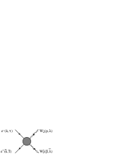
Figure 1: The process $e^{-}e^{+}\rightarrow W^{-}W^{+}$ with momentum and helicity assignments. The momenta $k$ and $\overline{k}$ are incoming, but $p$ and $\overline{p}$ are outgoing. The arrows on the $W$-boson lines indicate the flow of negative electric charge.

The four-momenta of the $e^{-}$, $e^{+}$, $W^{-}$ and $W^{+}$ are $k$, $\overline{k}$, $p$ and $\overline{p}$, respectively. The helicity of the $e^{-}$ ($e^{+}$) is given by $\frac{1}{2}\tau$ ($\frac{1}{2}\overline{\tau}$), and $\lambda$ ($\overline{\lambda}$) is the helicity of the $W^{-}$ ($W^{+}$) boson. In the limit of massless electrons only $\overline{\tau}=-\tau$ amplitudes survive, and the most general amplitude for this process may be written as [3]

$${\cal M}_{e^{-}e^{+}\rightarrow W^{-}W^{+}}(k,\overline{k},\tau;p,\overline{p},\lambda,\overline{\lambda})=\sum_{i=1}^{16}F_{i,\tau}(s,t)\,j_{\mu}(k,\overline{k},\tau)T_{i}^{\mu\alpha\beta}\epsilon_{\alpha}(p,\lambda)^{\ast}\epsilon_{\beta}(\overline{p},\overline{\lambda})^{\ast}\;,$$ (2.2)

where all dynamical information is contained in the scalar form-factors $F_{i,\tau}(s,t)$ with $s=(k+\overline{k})^{2}$ and $t=(k-p)^{2}$. The remaining factors on the right-hand side of Eqn. (2.2) are purely kinematical; $\epsilon_{\alpha}(p,\lambda)^{\ast}$ and $\epsilon_{\beta}(\overline{p},\overline{\lambda})^{\ast}$ are the polarization vectors for the $W^{-}$ and $W^{+}$ bosons, respectively, and $j_{\mu}(k,\overline{k},\tau)$ is the massless electron current,

$$j_{\mu}(k,\overline{k},\tau)=\overline{v}(\overline{k},-\tau)\gamma_{\mu}u(k,\tau)\;.$$ (2.3)

The summation over $i$ merits further discussion. The tensors, $T_{i}^{\mu\alpha\beta}$, have three independent Lorentz indices, and each Lorentz index may assume four values. Hence, one might expect that there are $4^{3}=64$ independent form factors. One factor of four corresponds to the degrees of freedom for the $W^{-}$ boson: three physical polarizations plus one unphysical degree of freedom. We refer to the physical polarizations as the transverse and longitudinal polarizations, and the unphysical degree of freedom is the scalar polarization. Likewise, for the $W^{+}$ boson there are three physical polarizations plus one unphysical scalar polarization. Finally, there are two ways to align plus two ways to anti-align the electron and positron helicities yielding the third factor of four. However, since we are working in the limit of massless electrons, we only need to consider the two helicity-aligned states, implying 32 independent form factors. We also find that one set of tensors may be used for both the left- and right-handed electron currents. Hence, the sum runs from $i=1$ to 16, and each form factor carries a subscript $\tau$.

The three physical polarization vectors are orthogonal to the momentum of the $W$ boson,

$$p_{\mu}\epsilon^{\mu}(p,\lambda)^{\ast}=\overline{p}_{\mu}\epsilon^{\mu}(\overline{p},\overline{\lambda})^{\ast}=0\;,$$ (2.4)

and the scalar polarization is defined proportional to momentum vector by

$$\epsilon^{\mu}(p,S)^{\ast}=\frac{p^{\mu}}{m_{W}}\;,\makebox[14.22636pt]{}\epsilon^{\mu}(\overline{p},S)^{\ast}=\frac{\overline{p}^{\mu}}{m_{W}}\;,$$ (2.5)

where $m_{W}$ is the physical mass of the $W$ boson. Hence the appearance of factors such as $p^{\alpha}$ and $\overline{p}^{\beta}$ in a tensor $T_{i}^{\mu\alpha\beta}$ indicate that its associated form factor contributes only for unphysical amplitudes. Furthermore, factors of $q^{\mu}$ do not survive due to current conservation, and factors of $k^{\mu}$ or $\overline{k}^{\mu}$ don’t survive due to the Dirac equation for massless fermions, i.e. $k\!\!\!/u(k)=0$ and $\overline{v}(\overline{k})\overline{k}\!\!\!/=0$. Then, the sixteen tensors may be chosen as

$$T_{1}^{\mu\alpha\beta} = P^{\mu}g^{\alpha\beta}\;,$$ (2.6a)

$$T_{2}^{\mu\alpha\beta} = \frac{-1}{m_{W}^{2}}P^{\mu}q^{\alpha}q^{\beta}\;,$$ (2.6b)

$$T_{3}^{\mu\alpha\beta} = q^{\alpha}g^{\mu\beta}-q^{\beta}g^{\alpha\mu}\;,$$ (2.6c)

$$T_{4}^{\mu\alpha\beta} = i\Big{(}q^{\alpha}g^{\mu\beta}+q^{\beta}g^{\alpha\mu}\Big{)}\;,$$ (2.6d)

$$T_{5}^{\mu\alpha\beta} = i\epsilon^{\mu\alpha\beta\rho}P_{\rho}\;,$$ (2.6e)

$$T_{6}^{\mu\alpha\beta} = -\epsilon^{\mu\alpha\beta\rho}q_{\rho}\;,$$ (2.6f)

$$T_{7}^{\mu\alpha\beta} = \frac{-1}{m_{W}^{2}}P^{\mu}\epsilon^{\alpha\beta\rho\sigma}q_{\rho}P_{\sigma}\;,$$ (2.6g)

$$T_{8}^{\mu\alpha\beta} = K^{\beta}g^{\alpha\mu}+K^{\alpha}g^{\mu\beta}\;,$$ (2.6h)

$$T_{9}^{\mu\alpha\beta} = \frac{i}{m_{W}^{2}}\Big{(}K^{\alpha}\epsilon^{\beta\mu\rho\sigma}+K^{\beta}\epsilon^{\alpha\mu\rho\sigma}\Big{)}q_{\rho}P_{\sigma}\;,$$ (2.6i)

$$T_{10}^{\mu\alpha\beta} = p^{\alpha}g^{\mu\beta}\;,$$ (2.6j)

$$T_{11}^{\mu\alpha\beta} = \frac{1}{m_{W}^{2}}P^{\mu}P^{\beta}p^{\alpha}\;,$$ (2.6k)

$$T_{12}^{\mu\alpha\beta} = \frac{i}{m_{W}^{2}}\epsilon^{\mu\beta\rho\sigma}P_{\rho}q_{\sigma}p^{\alpha}\;,$$ (2.6l)

$$T_{13}^{\mu\alpha\beta} = \overline{p}^{\beta}g^{\mu\alpha}\;,$$ (2.6m)

$$T_{14}^{\mu\alpha\beta} = \frac{1}{m_{W}^{2}}P^{\mu}P^{\alpha}\overline{p}^{\beta}\;,$$ (2.6n)

$$T_{15}^{\mu\alpha\beta} = \frac{i}{m_{W}^{2}}\epsilon^{\mu\alpha\rho\sigma}P_{\rho}q_{\sigma}\overline{p}^{\beta}\;,$$ (2.6o)

$$T_{16}^{\mu\alpha\beta} = \frac{1}{m_{W}^{2}}P^{\mu}p^{\alpha}\overline{p}^{\beta}\;,$$ (2.6p)

where

$$P = p-\overline{p}\;,$$ (2.7a)

$$q = k+\overline{k}=p+\overline{p}\;,$$ (2.7b)

$$K = k-\overline{k}\;,$$ (2.7c)

and $\epsilon_{0123}=-\epsilon^{0123}=+1$. We explicitly use the physical $W$-boson mass, $m_{W}$, in the definition of the tensors; this choice will be important when discussing one-loop corrections. Tensors $T_{1}^{\mu\alpha\beta}$ through $T_{9}^{\mu\alpha\beta}$, which were listed in Ref. [3], are sufficient to describe all physical amplitudes. The first seven tensors are sufficient to describe the most general $\gamma WW$ and $ZWW$ vertex functions [15]. Tensors $T_{10}^{\mu\alpha\beta}$ through $T_{12}^{\mu\alpha\beta}$ contribute if the $W^{-}$ boson has a scalar polarization, $T_{13}^{\mu\alpha\beta}$ through $T_{15}^{\mu\alpha\beta}$ contribute if the $W^{+}$ boson is unphysical, and $T_{16}^{\mu\alpha\beta}$ is needed only when both $W$ bosons have scalar polarizations.

2.2 $e^{+}e^{-}\rightarrow\chi^{+}W^{-}$ and $e^{+}e^{-}\rightarrow W^{+}\chi^{-}$

Next we consider amplitudes for $e^{+}e^{-}\rightarrow W^{\pm}\chi^{\mp}$. See Figs. 2(a) and 2(b).

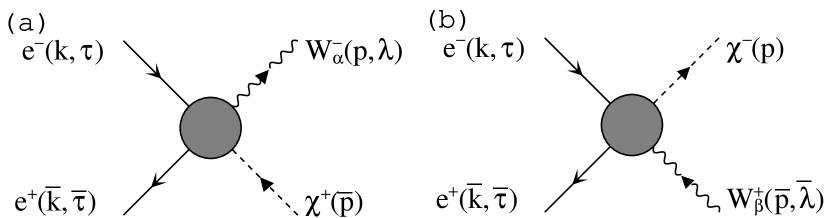
Figure 2: The processes (a) $e^{+}e^{-}\rightarrow W^{-}\chi^{+}$ and (b) $e^{+}e^{-}\rightarrow\chi^{-}W^{+}$ with momentum and helicity assignments chosen to coincide as closely as possible to those in Fig. 1. The momenta $k$ and $\overline{k}$ are incoming, but $p$ and $\overline{p}$ are outgoing. The arrows along the $W$-boson and Goldstone-boson lines indicate the flow of negative electric charge.

Our phase convention for the Goldstone bosons is that of Ref. [12]. We decompose the amplitudes as follows:

$${\cal M}_{e^{-}e^{+}\rightarrow W^{-}\chi^{+}}(k,\overline{k},\tau;p,\overline{p},\lambda) = i\sum_{i=1}^{4}H_{i,\tau}(s,t)\,j_{\mu}(k,\overline{k},\tau)S_{i}^{\mu\alpha}\epsilon_{\alpha}(p,\lambda)^{\ast}\;,$$ (2.8a)

$${\cal M}_{e^{-}e^{+}\rightarrow\chi^{-}W^{+}}(k,\overline{k},\tau;p,\overline{p},\overline{\lambda}) = i\sum_{i=1}^{4}\overline{H}_{i,\tau}(s,t)\,j_{\mu}(k,\overline{k},\tau)\overline{S}_{i}^{\mu\beta}\epsilon_{\beta}(\overline{p},\overline{\lambda})^{\ast}\;.$$ (2.8b)

There are four independent tensors, $S_{i}^{\mu\alpha}$, corresponding to the four polarizations, three physical plus one scalar, of the $W^{-}$ boson in $W^{-}\chi^{+}$ production, and each form factor $H_{i,\tau}(s,t)$ carries an index for the electron helicity, $\tau$. The tensors are given by

$$S_{1}^{\mu\alpha} = m_{W}g^{\mu\alpha}\;,$$ (2.9a)

$$S_{2}^{\mu\alpha} = \frac{1}{m_{W}}P^{\mu}P^{\alpha}\;,$$ (2.9b)

$$S_{3}^{\mu\alpha} = \frac{i}{m_{W}}\epsilon^{\mu\alpha\rho\sigma}P_{\rho}q_{\sigma}\;,$$ (2.9c)

$$S_{4}^{\mu\alpha} = \frac{1}{m_{W}}P^{\mu}p^{\alpha}\;,$$ (2.9d)

where $P^{\mu}$ and $q^{\mu}$ are given by Eqns. (2.7). The tensors $S_{1}^{\mu\alpha}$ through $S_{3}^{\mu\alpha}$ contribute to $W^{-}\chi^{+}$ production when the $W^{-}$ has a physical polarization, while $S_{4}^{\mu\alpha}$ contributes for the scalar polarization. A second set of four tensors is introduced for $W^{+}\chi^{-}$ production:

$$\overline{S}_{i}^{\mu\beta} = S_{i}^{\mu\beta}\makebox[17.07182pt]{}(i=1,2,3)\;,$$ (2.10a)

$$\overline{S}_{4}^{\mu\beta} = \frac{1}{m_{W}}P^{\mu}\overline{p}^{\beta}\;.$$ (2.10b)

$\overline{S}_{1}^{\mu\beta}$ through $\overline{S}_{3}^{\mu\beta}$ contribute for physical polarizations, and $\overline{S}_{4}^{\mu\beta}$ contributes for the scalar polarization of the $W^{+}$ boson. The corresponding form factors are given by $\overline{H}_{i,\tau}(s,t)$.

2.3 $e^{+}e^{-}\rightarrow\chi^{+}\chi^{-}$

The process $e^{+}e^{-}\rightarrow\chi^{+}\chi^{-}$ is shown in Fig. 3.

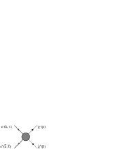
Figure 3: The process $e^{+}e^{-}\rightarrow\chi^{-}\chi^{+}$ with momentum and helicity assignments chosen to coincide as closely as possible to those in Fig. 1. The momenta $k$ and $\overline{k}$ are incoming, but $p$ and $\overline{p}$ are outgoing. The arrows along the Goldstone-boson lines indicate the flow of negative electric charge.

The corresponding amplitude may be decomposed as

$${\cal M}(e^{+}e^{-}\rightarrow\chi^{+}\chi^{-})=P^{\mu}j_{\mu}(k,\bar{k},\tau)R_{\tau}(s,t)\;.$$ (2.11)

Notice that there is only one form factor, $R_{\tau}(s,t)$, which carries an index for the electron helicity.

3 Applications of BRS Symmetry

Now that we have presented the form-factor decompositions for our diboson production amplitudes we can recast our single BRS identities of Eqns. (1.8a) and (1.8b) and our double BRS identity of Eqn. (1.9) as sum rules among the form factors. In this section we will also comment on the relationship between our exact sum rules and the equivalence theorem which only holds in the high-energy limit.

Before we proceed it is convenient to present the relationships between the rank-three tensors, $T_{i}^{\mu\alpha\beta}$, the rank-two tensors, $S_{i}^{\mu\alpha}$ and $\overline{S}_{i}^{\mu\beta}$, and the rank-one tensor, $P^{\mu}$, which were used in the decompositions of $e^{+}e^{-}\rightarrow W^{+}W^{-}$, $e^{+}e^{-}\rightarrow\chi^{\pm}W^{\mp}$ and $e^{+}e^{-}\rightarrow\chi^{+}\chi^{-}$ amplitudes. In general we can write

$$T_{i}^{\mu\alpha\beta}\epsilon_{\beta}(\bar{p},S)^{\ast} = \sum_{j=1}^{4}\xi_{ij}(s,t)S_{j}^{\mu\alpha}\;,$$ (3.1a)

$$T_{i}^{\mu\alpha\beta}\epsilon_{\alpha}(p,S)^{\ast} = \sum_{j=1}^{4}\overline{\xi}_{ij}(s,t)\overline{S}_{j}^{\mu\beta}\;,$$ (3.1b)

and

$$S_{j}^{\mu\alpha}\epsilon_{\alpha}(p,S)^{\ast} = \eta_{j}P^{\mu}\;,$$ (3.2a)

$$\overline{S}_{j}^{\mu\beta}\epsilon_{\beta}(\overline{p},S)^{\ast} = \overline{\eta}_{j}P^{\mu}\;.$$ (3.2b)

The coefficients $\xi_{ij}(s,t)$ and $\overline{\xi}_{ij}(s,t)$, which are dimensionless functions of the Mandelstam variables $s$ and $t$, are given in Table 1. In Table 2 we list the coefficients $\eta_{j}$ and $\overline{\eta}_{j}$. The expressions

$i$	$\xi_{i1}$	$\xi_{i2}$	$\xi_{i3}$	$\xi_{i4}$
$1$		$-1$		$1$
$2$		$2\gamma^{2}$		$-4\gamma^{2}$
$3$	$-2\gamma^{2}$	$1/2$		$-1$
$4$	$i2\gamma^{2}$	$i/2$		$-i$
$5$			$-1/2$
$6$			$-i/2$
$7$
$8$	$4\delta^{2}$		$-\tau/2$
$9$			$2\delta^{2}$
$10$				$-1/2$
$11$				$2\gamma^{2}-2$
$12$
$13$	$1$
$14$		$1$
$15$			$1$
$16$				$1$

$i$	$\overline{\xi}_{i1}$	$\overline{\xi}_{i2}$	$\overline{\xi}_{i3}$	$\overline{\xi}_{i4}$
$i$		$1$		$1$
$2$		$-2\gamma^{2}$		$-4\gamma^{2}$
$3$	$2\gamma^{2}$	$-1/2$		$-1$
$4$	$i2\gamma^{2}$	$i/2$		$i$
$5$			$1/2$
$6$			$-i/2$
$7$
$8$	$-4\delta^{2}$		$\tau/2$
$9$			$-2\delta^{2}$
$10$	$1$
$11$		$1$
$12$			$1$
$13$				$1/2$
$14$				$-2\gamma^{2}+2$
$15$
$16$				$1$

Table 1: The coefficients $\xi_{ij}(s,t)$ of Eqn. (3.1a) and $\overline{\xi}_{ij}(s,t)$ of Eqn. (3.1b). Only nonzero values are shown.

	$j=1$	$j=2$	$j=3$	$j=4$
$\eta_{j}$	$1/2$	$-2(\gamma^{2}-1)$	$0$	$1$
$\overline{\eta}_{j}$	$-1/2$	$2(\gamma^{2}-1)$	$0$	$1$

Table 2: The coefficients $\eta_{j}$ and $\overline{\eta}_{j}$ of Eqns. (3.2a) and (3.2b), respectively.

$$\gamma^{2} = \frac{s}{4m_{W}^{2}}\;,$$ (3.3a)

$$\delta^{2} = \frac{s+2t-2m_{W}^{2}}{4m_{W}^{2}}\;,$$ (3.3b)

are used in the tables.

3.1 ‘Single’ BRS sum rules

Because we frequently refer to the combinations of amplitudes which appear in the single BRS identities of Eqns. (1.8a) and (1.8b), it is convenient to define $G_{i,\tau}$ and $\overline{G}_{i,\tau}$ by

$$j_{\mu}(k,\overline{k},\tau)G_{j,\tau}S_{j}^{\mu\alpha}\epsilon_{\alpha}(p,\lambda)^{\ast} = {\cal M}(e^{+}e^{-}\rightarrow W^{-}_{P}W^{+}_{S})+i\,C_{\rm mod}{\cal M}(e^{+}e^{-}\rightarrow W^{-}_{P}\chi^{+})\;,$$ (3.4a)

$$j_{\mu}(k,\overline{k},\tau)\overline{G}_{j,\tau}\overline{S}_{j}^{\mu\beta}\epsilon_{\beta}(\overline{p},\overline{\lambda})^{\ast} = {\cal M}(e^{+}e^{-}\rightarrow W^{-}_{S}W^{+}_{P})+i\,C_{\rm mod}{\cal M}(e^{+}e^{-}\rightarrow\chi^{-}W^{+}_{P})\;.$$ (3.4b)

BRS symmetry then implies $G_{i,\tau}=\overline{G}_{i,\tau}=0$. Next, we rewrite Eqn. (2.2) requiring that the $W^{+}$ boson has an unphysical scalar polarization and the $W^{-}$ is physical. Employing the expansion of Eqn. (3.1a) we obtain

$${\cal M}(e^{+}e^{-}\rightarrow W^{-}_{P}W^{+}_{S})=\sum_{j=1}^{3}\left\{\sum_{i=1}^{16}\xi_{ij}(s,t)F_{i,\tau}(s,t)\right\}j_{\mu}(k,\bar{k},\tau)S_{j}^{\mu\alpha}\epsilon_{\alpha}(p,P)^{\ast}\;,$$ (3.5)

where $S_{4}^{\mu\alpha}$ does not contribute by Eqn. (2.4). If we insert this expression along with the expansion of the $e^{+}e^{-}\rightarrow W^{-}\chi^{+}$ amplitude of Eqn. (2.8a) into Eqn. (1.8a), then we find the following sum rules:

$$G_{j,\tau}(s,t)=\sum_{i=1}^{16}F_{i,\tau}(s,t)\xi_{ij}(s,t)-C_{\rm mod}H_{j,\tau}(s,t)=0\;,$$ (3.6)

for $j=1,2,3$. In a parallel fashion, if we rewrite Eqn. (2.2) for a physical $W^{+}$ boson and an unphysical $W^{-}$, then applying Eqn. (3.1b) yields

$${\cal M}(e^{+}e^{-}\rightarrow W^{-}_{S}W^{+}_{P})=\sum_{j=1}^{3}\left\{\sum_{i=1}^{16}\overline{\xi}_{ij}(s,t)F_{i,\tau}(s,t)\right\}j_{\mu}(k,\bar{k},\tau)\overline{S}_{j}^{\mu\beta}\epsilon_{\beta}(\overline{p},P)^{\ast}.$$ (3.7)

We insert this in Eqn. (1.8b) along with Eqn. (2.8b) to obtain

$$\overline{G}_{j,\tau}(s,t)=\sum_{i=1}^{16}F_{i,\tau}(s,t)\overline{\xi}_{ij}(s,t)-C_{\rm mod}\overline{H}_{j,\tau}(s,t)=0\;,$$ (3.8)

for $j=1,2,3$.

Inserting the coefficients $\xi_{ij}$ as listed in Table 1 we write

$$\!\!\!\!-2\gamma^{2}\,\Big{\{}F_{3,\tau}(s,t)-i\,F_{4,\tau}(s,t)\Big{\}}+4\delta^{2}\,F_{8,\tau}(s,t)+F_{13,\tau}(s,t)-C_{\rm mod}H_{1,\tau}(s,t) = 0\;,\;\;$$ (3.9a)

$$\!\!\!\!-F_{1,\tau}(s,t)+2\gamma^{2}\,F_{2,\tau}(s,t)+\frac{1}{2}F_{3,\tau}(s,t)+\frac{i}{2}F_{4,\tau}(s,t)+F_{14,\tau}(s,t)-C_{\rm mod}H_{2,\tau}(s,t) = 0\;,\;\;$$ (3.9b)

$$\!\!\!\!-\frac{1}{2}F_{5,\tau}(s,t)-\frac{i}{2}F_{6,\tau}(s,t)-\frac{\tau}{2}F_{8,\tau}(s,t)+2\delta^{2}\,F_{9,\tau}(s,t)+F_{15,\tau}(s,t)-C_{\rm mod}H_{3,\tau}(s,t) = 0\;,\;\;$$ (3.9c)

corresponding to $G_{1,\tau}=0$, $G_{2,\tau}=0$ and $G_{3,\tau}=0$, respectively. Taking the $\overline{\xi}_{ij}$ from Table 1 produces

$$\!\!\!\!2\gamma^{2}\Big{\{}F_{3,\tau}(s,t)+i\,F_{4,\tau}(s,t)\Big{\}}-4\delta^{2}\,F_{8,\tau}(s,t)+F_{10,\tau}(s,t)-C_{\rm mod}\overline{H}_{1,\tau}(s,t) = 0\;,\;\;$$ (3.10a)

$$\!\!\!\!F_{1,\tau}(s,t)-2\gamma^{2}\,F_{2,\tau}(s,t)-\frac{1}{2}F_{3,\tau}(s,t)+\frac{i}{2}F_{4,\tau}(s,t)+F_{11,\tau}(s,t)-C_{\rm mod}\overline{H}_{2,\tau}(s,t) = 0\;,\;\;$$ (3.10b)

$$\!\!\!\!\frac{1}{2}F_{5,\tau}(s,t)-\frac{i}{2}F_{6,\tau}(s,t)+\frac{\tau}{2}F_{8,\tau}(s,t)-2\delta^{2}\,F_{9,\tau}(s,t)+F_{12,\tau}(s,t)-C_{\rm mod}\overline{H}_{3,\tau}(s,t) = 0\;.\;\;$$ (3.10c)

corresponding to $\overline{G}_{j,\tau}=0$ for $j=1,2,3$. Note that the expression of these sum rules holds for each order of the perturbative expansion. Eqns. (3.9a)-(3.9c), taking into account the two electron helicity states, are a set of six sum rules. Of the eighteen form factors that contribute to physical $W$-boson pair production amplitudes, i.e. $F_{1,\tau}$ through $F_{9,\tau}$, all but the CP-violating $F_{7,\tau}$ appear. ($F_{7,\tau}$ only contributes to final states where both $W$ bosons have the same transverse polarization, hence cannot contribute to these sum rules.) In order to test via Eqns. (3.9a)-(3.9c) the remaining sixteen, we must also retain $F_{10,\tau}$ through $F_{12,\tau}$ in the evaluation of the $e^{+}e^{-}\rightarrow W^{+}W^{-}$ amplitudes. It is furthermore necessary to obtain $H_{1,\tau}$ through $H_{3,\tau}$ from the independent evaluation of the $e^{+}e^{-}\rightarrow\chi^{+}W^{-}$ amplitudes. The test is extremely powerful and hence worthy of the extra effort. Each form factor can have its own complicated dependence on $s$ and $t$. Each can include a large number of loop diagrams. Yet when added together they satisfy the above sum rules.

Eqns. (3.10a)-(3.10c) yield an additional set of six sum rules which again test all of the physically relevant form factors except $F_{7,\tau}$. In this case we must retain $F_{13,\tau}$ through $F_{15,\tau}$ in the evaluation of the $e^{+}e^{-}\rightarrow W^{+}W^{-}$ amplitudes while obtaining $\overline{H}_{1,\tau}$ through $\overline{H}_{3,\tau}$ from the evaluation of the $e^{+}e^{-}\rightarrow W^{+}\chi^{-}$ amplitudes. As a practical matter, once one set of sum rules, either Eqns. (3.9a)-(3.9c) or Eqns. (3.10a)-(3.10c), is used to verify the accuracy of a calculation, the other set is redundant.

3.2 ‘Double’ BRS Sum rules

Next we rewrite Eqn. (2.2) requiring that both $W$ bosons have unphysical scalar polarizations. Then we can use Eqn. (3.1a) followed by Eqn. (3.2a), or we can use Eqn. (3.1b) followed by Eqn. (3.2b) to obtain

$${\cal M}(e^{+}e^{-}\rightarrow W^{+}_{S}W^{-}_{S}) = P^{\mu}j_{\mu}(k,\bar{k},\tau)\sum_{j=1}^{4}\sum_{i=1}^{16}F_{i,\tau}(s,t)\xi_{ij}(s,t)\eta_{j}$$ (3.11)

$$= P^{\mu}j_{\mu}(k,\bar{k},\tau)\sum_{j=1}^{4}\sum_{i=1}^{16}F_{i,\tau}(s,t)\bar{\xi}_{ij}(s,t)\bar{\eta}_{j}\;.$$

Then, from Eqns. (2.8a) and (2.8b), we have

$${\cal M}(e^{+}e^{-}\rightarrow\chi^{+}W^{-}_{S}) = iP^{\mu}j_{\mu}(k,\bar{k},\tau)\sum_{j}^{4}H_{j,\tau}(s,t)\,\eta_{j}\;,$$ (3.12a)

$${\cal M}(e^{+}e^{-}\rightarrow W^{+}_{S}\chi^{-}) = iP^{\mu}j_{\mu}(k,\bar{k},\tau)\sum_{j}^{4}\overline{H}_{j,\tau}(s,t)\,\overline{\eta}_{j}\;.$$ (3.12b)

Incorporating the expansion of the $e^{+}e^{-}\rightarrow\chi^{+}\chi^{-}$ amplitude in Eqn. (2.11), the double BRS identity of Eqn. (1.9) becomes

$$\!\!\!\!\!\!\!\!\!\!\!\!\!\!\!\!\!\!\!\!\sum_{i=1}^{16}F_{i,\tau}(s,t)\xi_{ij}(s,t)\eta_{j}-C_{\rm mod}\sum_{j=1}^{4}H_{j,\tau}(s,t)\eta_{j}-C_{\rm mod}\sum_{j=1}^{4}\overline{H}_{j,\tau}(s,t)\overline{\eta}_{j}-\left\{C_{\rm mod}\right\}^{2}R_{\tau}(s,t) = 0\;,$$ (3.13a)

$$\!\!\!\!\!\!\!\!\!\!\!\!\!\!\!\!\!\!\!\ \sum_{i=1}^{16}F_{i,\tau}(s,t)\overline{\xi}_{ij}(s,t)\overline{\eta}_{j}-C_{\rm mod}\sum_{j=1}^{4}H_{j,\tau}(s,t)\eta_{j}-C_{\rm mod}\sum_{j=1}^{4}\overline{H}_{j,\tau}(s,t)\overline{\eta}_{j}-\left\{C_{\rm mod}\right\}^{2}R_{\tau}(s,t) = 0\;.$$ (3.13b)

3.3 Relationship to the equivalence theorem

Here, we would like to comment on the relationship between the BRS sum rules and the equivalence theorem[8, 9, 10]. The theorem states that the amplitudes for a process with longitudinally polarized gauge bosons $W_{L}^{\pm}$ are equivalent at energies where $s\gg m_{W}^{2}$ to those of the process in which the $W_{L}^{\pm}$ bosons are replaced by their corresponding Goldstone bosons. The theorem follows from BRS symmetry and the equivalence of the longitudinal and scalar polarization vectors at high energies. Consider $W$-boson pair production in the center of momentum frame with the $W^{-}$ boson momentum along the positive $z$ axis. In this frame the longitudinal and scalar polarization vectors are given by

$$\epsilon^{\mu}(p,0)^{\ast} = \gamma\Big{(}\beta,0,0,1\Big{)}\;,$$ (3.14a)

$$\epsilon^{\mu}(p,S)^{\ast} = \gamma\Big{(}1,0,0,\beta\Big{)}\;,$$ (3.14b)

$$\epsilon^{\mu}(\overline{p},0)^{\ast} = \gamma\Big{(}\beta,0,0,-1\Big{)}\;,$$ (3.14c)

$$\epsilon^{\mu}(\overline{p},S)^{\ast} = \gamma\Big{(}1,0,0,-\beta\Big{)}\;.$$ (3.14d)

Thus for energies large compared to the $W$-boson mass we have

$$\epsilon^{\mu}(p,0)^{\ast} = \epsilon^{\mu}(p,S)^{\ast}\left(1+{\cal O}(m_{W}/\sqrt{s})\right)\;,$$ (3.15a)

$$\epsilon^{\mu}(\overline{p},0)^{\ast} = \epsilon^{\mu}(\overline{p},S)^{\ast}\left(1+{\cal O}(m_{W}/\sqrt{s})\right)\;.$$ (3.15b)

Hence we may rewrite the ‘single’ BRS identities of Eqns. (1.8a) and (1.8b) to find

$${\cal M}\Big{(}e^{+}e^{-}\rightarrow W^{-}_{L}\,W^{+}_{L}\Big{)} = -iC_{\rm mod}{\cal M}\Big{(}e^{+}e^{-}\rightarrow W^{-}_{L}\,\chi^{+}\Big{)}\,\left(1+{\cal O}(m_{W}/\sqrt{s})\right)\;,$$ (3.16a)

$${\cal M}\Big{(}e^{+}e^{-}\rightarrow W^{-}_{L}\,W^{+}_{L}\Big{)} = -iC_{\rm mod}{\cal M}\Big{(}e^{+}e^{-}\rightarrow\chi^{-}\,W^{+}_{L}\Big{)}\,\left(1+{\cal O}(m_{W}/\sqrt{s})\right)\;,$$ (3.16b)

while, for the double BRS identity of Eqn. (1.9), we obtain

$${\cal M}(e^{+}e^{-}\rightarrow W^{+}_{L}\,W^{-}_{L})+iC_{\rm mod}{\cal M}(e^{+}e^{-}\rightarrow W^{+}_{L}\,\chi^{-})$$

$$\makebox[14.22636pt]{}+iC_{\rm mod}{\cal M}(e^{+}e^{-}\rightarrow\chi^{+}\,W^{-}_{L})=\left\{C_{\rm mod}\right\}^{2}{\cal M}(e^{+}e^{-}\rightarrow\chi^{+}\,\chi^{-})\,\left(1+{\cal O}(m_{W}/\sqrt{s})\right)\;.$$ (3.17)

Inserting Eqns. (3.16a) and (3.16b) into Eqn. (3.17), we obtain

$${\cal M}\Big{(}e^{+}e^{-}\rightarrow W^{-}_{L}\,W^{+}_{L}\Big{)} = \left\{-iC_{\rm mod}\right\}^{2}{\cal M}\Big{(}e^{+}e^{-}\rightarrow\chi^{-}\,\chi^{+}\Big{)}\,\left(1+{\cal O}\left(m_{W}/\sqrt{s}\right)\right)\;.$$ (3.18)

Although the equivalence theorem has often been used to check the consistency of various calculations (for example, see Ref. [18]), it is valid only in the high-energy limit. On the other hand, our BRS sum rules hold exactly at all energies. Therefore, where perturbation theory is applicable, BRS sum rules are a more powerful tool.

4 Calculation of the form factors in perturbation theory

In later sections we will present detailed one-loop calculations concerning $e^{+}e^{-}\rightarrow W^{+}W^{-}$ and $e^{+}e^{-}\rightarrow W^{\pm}\chi^{\mp}$ amplitudes. We will then check the calculation by using the BRS sum rules. Hence, in this section we present a discussion of the related form factors.

It is extremely important that we avoid any inconsistent treatment of higher order effects. Because we want to employ the physical $W$-boson mass we choose $m_{W}$ as one of our input parameters. We also choose $\hat{e}$ and $\hat{s}$, the ${\overline{\rm MS}}$ parameters of the electric coupling constant and sine of the Weinberg angle, respectively. These three parameters are consistently employed in the evaluation of all loop integrals and form factors. The ${\overline{\rm MS}}$ weak coupling constants $\hat{g}$ and $\hat{g}_{Z}$ are related to $\hat{e}$ and $\hat{s}$ by

$$\hat{c}^{2}=1-\hat{s}^{2},\;\;\hat{e}=\hat{g}\hat{s}=\hat{g}_{Z}\hat{s}\hat{c}\;.$$ (4.1)

The ${\overline{\rm MS}}$ masses of the massive gauge bosons are defined in terms of $\hat{e}$, $\hat{s}$ and $m_{W}$ by

$$\hat{m}_{W}^{2} = m_{W}^{2}+\Pi_{T}^{WW}(m_{W}^{2})\;,$$ (4.2)

$$\hat{m}_{Z}^{2} = \frac{\hat{m}_{W}^{2}}{\hat{c}^{2}}=\frac{1}{\hat{c}^{2}}\left\{m_{W}^{2}+\Pi_{T}^{WW}(m_{W}^{2})\right\}\;,$$ (4.3)

and the physical mass of the $Z$ boson is obtained (at the one-loop level) by

$$m_{Z}^{2}=\frac{m_{W}^{2}}{\hat{c}^{2}}+\frac{1}{\hat{c}^{2}}\Pi_{T}^{WW}(m_{W}^{2})-\Pi_{T}^{ZZ}\left(\frac{m_{W}^{2}}{\hat{c}^{2}}\right)\equiv\frac{m_{W}^{2}}{\hat{c}^{2}}+\Delta\;,$$ (4.4)

where the contributions of the two-point functions are represented by $\Delta$. Finally, when $m_{Z}^{2}$ appears in the denominator we perform an expansion and truncate after the term which is linear in $\Delta$ as

$$\frac{1}{s-m_{Z}^{2}}=\frac{1}{s-(m_{W}^{2}/\hat{c}^{2})}\left\{1+\frac{\Delta}{s-m_{W}^{2}/\hat{c}^{2}}\right\}\;.$$ (4.5)

In Ref. [16], we will demonstrate that, by following this scheme, we are able to satisfy the BRS sum rules to the limit of floating-point prescription.

4.1 $e^{+}e^{-}\rightarrow W^{+}W^{-}$

The form factors $F_{i,\tau}(s,t)$ which were introduced in Eqn. (2.2) may be written as

$$\makebox[-28.45274pt]{}F_{i,\tau}(s,t)=\frac{\hat{e}^{2}}{s}\Bigg{\{}\bigg{[}Q_{e}\Big{(}1-{\Pi}_{T,\gamma}^{\gamma\gamma}(s)+\Gamma_{1}^{\,e}(s)\Big{)}+T^{3}_{e}\,\overline{\Gamma}\mbox{}^{\,e}_{2}(s)\bigg{]}f_{i}^{\gamma\,(0)}+Q_{e}f_{i}^{\gamma\,(1)}(s)\Bigg{\}}$$

$$\makebox[-14.22636pt]{}+\frac{\hat{g}^{2}}{s-(m_{W}^{2}/\hat{c}^{2})}\Bigg{\{}\bigg{[}\big{(}T^{3}_{e}-\hat{s}^{2}Q_{e}\big{)}\Big{(}1+\frac{\Delta}{s-m_{W}^{2}/\hat{c}^{2}}-{\Pi}_{T,Z}^{ZZ}(s)+\Gamma_{1}^{\,e}(s)\Big{)}+T^{3}_{e}\Big{(}\hat{c}^{2}\overline{\Gamma}_{2}^{\,e}(s)+\Gamma_{3}^{\,e}(s)\Big{)}$$

$$\makebox[45.52458pt]{}+\Gamma_{4}^{\,e}(s)\bigg{]}f_{i}^{Z\,(0)}+\big{(}T^{3}_{e}-\hat{s}^{2}Q_{e}\big{)}f_{i}^{Z\,(1)}(s)-\frac{\hat{s}}{\hat{c}}\bigg{[}Q_{e}\hat{c}^{2}f_{i}^{Z\,(0)}+\big{(}T^{3}_{e}-\hat{s}^{2}Q_{e}\big{)}f_{i}^{\gamma\,(0)}\bigg{]}{\Pi}_{T,\gamma}^{\gamma Z}(s)\Bigg{\}}$$

$$\makebox[-14.22636pt]{}+\frac{T^{3}_{e}\hat{g}^{2}}{2t}\Big{[}f_{i}^{t\,(0)}+\Gamma^{e\nu W}(t)+\overline{\Gamma}^{e\nu W}(t)\Big{]}+F_{i,\tau}^{[\rm Box]}(s,t)\;,$$ (4.6)

where the electric charge and the third component of weak isospin of the electron are given by $Q_{e}=-1$ and $T^{3}_{e}$, respectively. For left-handed electrons $T^{3}_{e}=-\frac{1}{2}$, and $T^{3}_{e}=0$ for right-handed electrons. We have already expanded the $Z$-boson propagator according to Eqn. (4.5). The other factors in Eqn. (4.6) are explained in the text below.

The tree-level $e^{+}e^{-}\rightarrow W^{+}W^{-}$ Feynman diagrams are shown in Fig. 4.

Figure 4: Tree-level Feynman diagrams for $e^{+}e^{-}\rightarrow W^{+}W^{-}$. The arrows on the $W$-boson lines indicate the flow of negative electric charge

Neglecting loop contributions the poles in $1/s$, $1/(s-m_{Z}^{2})$ and $1/t$ in Eqn. (4.6) correspond to the $s$-channel photon exchange, $s$-channel $Z$-boson exchange and $t$-channel neutrino exchange graphs, respectively. The appearance of the ${\Pi}_{T,\gamma}^{\gamma Z}$ term indicates $\gamma-Z$ mixing in the neutral current (NC) sector. In general we define

$$\Pi^{V_{1}V_{2}}_{T,V_{3}}({q^{2}})=\frac{\Pi^{V_{1}V_{2}}_{T}({q^{2}})-\Pi^{V_{1}V_{2}}_{T}(m^{2}_{V_{3}})}{{q^{2}}-m^{2}_{V_{3}}}\;,$$ (4.7)

which reduces to a derivative in the limit $m^{2}_{V_{3}}\rightarrow q^{2}$. Such an expression appears naturally when expanding a full propagator about the pole in the transverse part of the one-particle irreducible propagator function.

Our Feynman rules for the $WW\gamma$ and $WWZ$ vertices are written as

$$-i\hat{e}\sum_{i=1}^{16}f^{\gamma}_{i}T_{i}^{\mu\alpha\beta}\makebox[85.35826pt]{\rm and}-i\hat{g}_{Z}\hat{c}^{2}\sum_{i=1}^{16}f^{Z}_{i}T_{i}^{\mu\alpha\beta}\;,$$ (4.8)

respectively. This introduces the vertex form factors $f^{\gamma}_{i}$ and $f^{Z}_{i}$. The $t$-channel term is also expanded in the same $T_{i}^{\mu\alpha\beta}$ tensors yielding the form factors $f^{t}_{i}$. In turn each of these form factors is split into its tree-level value plus a one-loop correction as

$$f_{i}^{V}=f_{i}^{V\,(0)}+f_{i}^{V\,(1)}\;,$$ (4.9)

where $V=\gamma$ and $Z$. The nonzero tree-level values are given in Table 3.

i	1	2	3	4	5	6	7	8	9	10	11	12	13	14	15	16
$f_{i}^{\gamma\,(0)}$	1		2							$-1$			1
$f_{i}^{Z\,(0)}$	1		2							$-1$			1
$f_{i}^{t\,(0)}$	1		2		1			1		$-2$			2

Table 3: Explicit values for the $f_{i}^{X\,(0)}$ form factors of the SM at the tree level. Only nonzero values are shown.

Please note that $T_{8}^{\mu\alpha\beta}$ and $T_{9}^{\mu\alpha\beta}$ are precluded from contributing to the vector-boson vertex functions by angular momentum considerations[12]. One-loop corrections to the $WW\gamma$ vertex are then contained in the $f_{i}^{\gamma\,(1)}$ along with the $Z$ factors for the external $W$ bosons, $Z_{W}^{1/2}$, which multiply the corresponding $f_{i}^{\gamma\,(0)}$. Similarly, one-loop corrections to the $WWZ$ vertex along with the $Z_{W}^{1/2}$ factors that multiply the tree-level $WWZ$ vertex are contained in the $f_{i}^{Z(1)}$. The vertex functions for the $Vee$ vertex, denoted by $\Gamma_{1}^{\,e}$, $\overline{\Gamma}\mbox{}^{\,e}_{2}$, $\Gamma_{3}^{\,e}$ and $\Gamma_{4}^{\,e}$ also appear in $e^{+}e^{-}\rightarrow f\overline{f}$ amplitudes[17]; the corrections from the external electron two-point functions are absorbed into $\Gamma_{1}$. The vertex functions $\Gamma^{\,e\nu W}$ and $\overline{\Gamma}\mbox{}^{\,e\nu W}$ appear in charged current processes; they contain $\nu eW$ vertex corrections as well as two-point function corrections for the external electrons and $W$ bosons and the internal neutrino propagator. Finally, the $F_{i,\tau}^{[\rm Box]}$ terms account for contributions of box diagrams.

4.2 $e^{+}e^{-}\rightarrow\chi^{+}W^{-}$ and $e^{+}e^{-}\rightarrow W^{+}\chi^{-}$

We are not interested, per se, in the form factors $H_{i,\tau}(s,t)$ of Eqn. (2.8a) and $\overline{H}_{i,\tau}(s,t)$ of Eqn. (2.8b). Rather we are interested in $C_{\rm mod}{\stackrel{{\scriptstyle{\scriptscriptstyle(}-{\scriptscriptstyle)}}}{{H}}}_{i,\tau}(s,t)$ which is the expression that appears in the sum rules. Because $Z_{W}^{1/2}Z_{\chi}^{1/2}=1$, Eqn. (1.7) simplifies to

$$C_{\rm mod}=Z_{m}=\frac{\hat{m}_{W}}{m_{W}}\;.$$ (4.10)

Then we may compactly write

$$C_{\rm mod}\hbox to0.0pt{$\displaystyle{\stackrel{{\scriptstyle{\scriptscriptstyle(}-{\scriptscriptstyle)}}}{{H}}}\mbox{}_{i,\tau}(s,t)=\frac{\hat{e}^{2}}{s}\Bigg{\{}\bigg{[}Q_{e}\Big{(}\frac{\hat{m}_{W}^{2}}{m_{W}^{2}}-{\Pi}_{T,\gamma}^{\gamma\gamma}(s)+\Gamma_{1}^{\,e}(s)\Big{)}+T^{3}_{e}\overline{\Gamma}\mbox{}^{\,e}_{2}(s)\bigg{]}{\stackrel{{\scriptstyle{\scriptscriptstyle(}-{\scriptscriptstyle)}}}{{h}}}\mbox{}_{i}^{\gamma\,(0)}+Q_{e}{\stackrel{{\scriptstyle{\scriptscriptstyle(}-{\scriptscriptstyle)}}}{{h}}}\mbox{}_{i}^{\gamma\,(1)}(s)\Bigg{\}}$\hss}$$

$$\makebox[-42.67912pt]{}+\frac{\hat{g}^{2}}{s-m_{W}^{2}/\hat{c}^{2}}\Bigg{\{}\bigg{[}(T^{3}_{e}-\hat{s}^{2}Q_{e})\Big{(}\frac{\hat{m}_{W}^{2}}{m_{W}^{2}}+\frac{\Delta}{s-m_{W}^{2}/\hat{c}^{2}}-{\Pi}_{T,Z}^{ZZ}(s)+\Gamma_{1}^{\,e}(s)\Big{)}+T^{3}_{e}\Big{(}\hat{c}^{2}\overline{\Gamma}_{2}^{\,e}(s)+\Gamma_{3}^{\,e}(s)\Big{)}$$

$$\makebox[-42.67912pt]{}+\Gamma_{4}^{\,e}(s)\bigg{]}{\stackrel{{\scriptstyle{\scriptscriptstyle(}-{\scriptscriptstyle)}}}{{h}}}\mbox{}_{i}^{Z\,(0)}+(T^{3}_{e}-\hat{s}^{2}Q_{e}){\stackrel{{\scriptstyle{\scriptscriptstyle(}-{\scriptscriptstyle)}}}{{h}}}\mbox{}_{i}^{Z\,(1)}(s)-\frac{\hat{s}}{\hat{c}}\bigg{[}(T^{3}_{e}-\hat{s}^{2}Q_{e}){\stackrel{{\scriptstyle{\scriptscriptstyle(}-{\scriptscriptstyle)}}}{{h}}}\mbox{}_{i}^{\gamma\,(0)}+Q_{e}\hat{c}^{2}{\stackrel{{\scriptstyle{\scriptscriptstyle(}-{\scriptscriptstyle)}}}{{h}}}\mbox{}_{i}^{Z\,(0)}\bigg{]}{\Pi}_{T,\gamma}^{\gamma Z}(s)\Bigg{\}}+{\stackrel{{\scriptstyle{\scriptscriptstyle(}-{\scriptscriptstyle)}}}{{H}}}\mbox{}_{i,\tau}^{\,{\rm[Box]}}(s,t)\;.$$

At the tree level there are two Feynman graphs as shown in Fig. 5;

Figure 5: Tree-level Feynman diagrams contributing to $e^{+}e^{-}\rightarrow W^{-}\chi^{+}$. The arrows on the charged bosons indicate the flow of negative electric charge. By reversing the direction of these arrows we obtain the graphs for $e^{+}e^{-}\rightarrow W^{+}\chi^{-}$.

in the limit of massless electrons there is no $t$-channel graph. The discussion of the hatted couplings, the pole mass and the two-point function corrections follow those of the previous section. The expansion of $H_{i,\tau}(s,t)$ introduces the vertex form factors $h_{i}^{\gamma}$ and $h_{i}^{Z}$, while the expansion of $\overline{H}_{i,\tau}(s,t)$ introduces $\overline{h}_{i}^{\gamma}$ and $\overline{h}_{i}^{Z}$. The corresponding $VW^{\mp}\chi^{\pm}$ vertices are then expressed as

$$\hat{e}\sum_{i=1}^{4}h_{i}^{\gamma}S_{i}^{\mu\alpha}\;,\makebox[28.45274pt]{}\hat{g}_{Z}\hat{c}^{2}\sum_{i=1}^{4}h_{i}^{Z}S_{i}^{\mu\alpha}\;,\makebox[28.45274pt]{}\hat{e}\sum_{i=1}^{4}\overline{h}_{i}^{\,\gamma}\overline{S}_{i}^{\mu\beta}\;,\makebox[28.45274pt]{}\hat{g}_{Z}\hat{c}^{2}\sum_{i=1}^{4}\overline{h}_{i}^{Z}\overline{S}_{i}^{\mu\beta}\;.$$ (4.12)

We use the physical mass in defining our tensors while the $VW^{\pm}\chi^{\mp}$ coupling depends explicitly on $\hat{m}_{W}$. As before, the vertex form factors are written as the sum of the tree-level and one-loop contributions by

$${\stackrel{{\scriptstyle{\scriptscriptstyle(}-{\scriptscriptstyle)}}}{{h}}}\mbox{}_{i}^{V}(s)={\stackrel{{\scriptstyle{\scriptscriptstyle(}-{\scriptscriptstyle)}}}{{h}}}\mbox{}_{i}^{V\,(0)}\frac{\hat{m}_{W}}{m_{W}}+{\stackrel{{\scriptstyle{\scriptscriptstyle(}-{\scriptscriptstyle)}}}{{h}}}\mbox{}_{i}^{V\,(1)}\;,$$ (4.13)

for $V=\gamma$, $Z$. This explains the appearance of one power of the ratio of the $\overline{\rm MS}$ $W$-boson mass to the physical mass multiplying the leading-order term. The other power comes from $C_{\rm mod}$ as in Eqn. (4.10). The tree-level form-factor coefficients may be found in Table 4. The ${\stackrel{{\scriptstyle{\scriptscriptstyle(}-{\scriptscriptstyle)}}}{{h}}}\mbox{}_{i}^{V\,(1)}$ contain not only vertex corrections for the $VW\chi$ vertices but also the correction factors for the external $W$ bosons.

i	1	2	3	4		i	1	2	3	4
$h_{i}^{\gamma\,(0)}$	$1$					$\overline{h}_{i}^{\,\gamma\,(0)}$	$-1$
$h_{i}^{Z\,(0)}$	$-\hat{s}^{2}/\hat{c}^{2}$					$\overline{h}_{i}^{Z\,(0)}$	$\hat{s}^{2}/\hat{c}^{2}$

Table 4: Explicit values for the nonzero $h_{i}^{V\,(0)}$ and $\overline{h}_{i}^{V\,(0)}$ form factors of the SM at the tree level.

5 BRS Sum Rules at the tree level

Before we embark on the study of the BRS sum rules at the loop level it is instructive to first study them at the tree level. We first consider the sum rule in Eqn. (3.10a). We obtain the tree-level form factors from Eqns. (4.6) and (LABEL:big-H) by retaining only the Born term and setting $m_{Z}=\hat{m}_{Z}$ and $m_{W}=\hat{m}_{W}$. Then,

$$\overline{G}_{1,\tau} = 2\gamma^{2}\bigg{\{}2\frac{Q_{e}\hat{e}^{2}}{s}+2\frac{(T^{3}_{e}-\hat{s}^{2}Q_{e})\hat{g}_{Z}^{2}\hat{c}^{2}}{s-\hat{m}_{Z}^{2}}+2\frac{T^{3}_{e}\hat{g}^{2}}{2t}\bigg{\}}-4\delta^{2}\bigg{\{}\frac{T^{3}_{e}\hat{g}^{2}}{2t}\bigg{\}}$$ (5.1)

$$\mbox{}-\bigg{\{}\frac{Q_{e}\hat{e}^{2}}{s}+\frac{(T^{3}_{e}-\hat{s}^{2}Q_{e})\hat{g}_{Z}^{2}\hat{c}^{2}}{s-\hat{m}_{Z}^{2}}+2\frac{T^{3}_{e}\hat{g}^{2}}{2t}\bigg{\}}-\bigg{\{}-\frac{Q_{e}\hat{e}^{2}}{s}+\frac{(T^{3}_{e}-\hat{s}^{2}Q_{e})\hat{g}_{Z}^{2}\hat{s}^{2}}{s-\hat{m}_{Z}^{2}}\bigg{\}}\;.$$

Reading from left to right the four terms correspond to the contributions of $F_{3,\tau}$, $F_{8,\tau}$, $F_{10,\tau}$ and $\overline{H}_{1,\tau}$; $F_{4,\tau}$ also contributes but is identically zero at the tree-level. See Table 3. Regrouping the terms by electron quantum numbers yields

$$\overline{G}_{1,\tau} = Q_{e}\hat{e}^{2}\Bigg{\{}4\gamma^{2}\bigg{[}\frac{1}{s}-\frac{1}{s-\hat{m}_{Z}^{2}}\bigg{]}-\bigg{[}\frac{1}{s}-\frac{1}{s-\hat{m}_{Z}^{2}}\bigg{]}+\bigg{[}\frac{1}{s}+\frac{1}{s-\hat{m}_{Z}^{2}}\frac{\hat{s}^{2}}{\hat{c}^{2}}\bigg{]}\Bigg{\}}$$ (5.2)

$$\mbox{}+T^{3}_{e}\hat{g}^{2}\Bigg{\{}\Big{(}4\gamma^{2}-4\delta^{2}-2\Big{)}\frac{1}{2t}+\Big{(}4\gamma^{2}-1-\frac{\hat{s}^{2}}{\hat{c}^{2}}\Big{)}\frac{1}{s-\hat{m}_{Z}^{2}}\Bigg{\}}\;.$$

The coefficient of the pole in $1/t$ comes entirely from the neutrino-exchange diagram in $W$-boson pair production. We notice that $-4\gamma^{2}+4\delta^{2}+2=2t/\hat{m}_{W}^{2}$, and hence the dependence on $t$ cancels between the various $W$-pair contributions. After some simplification we find

$$\overline{G}_{1,\tau} = -\Big{\{}Q_{e}\hat{e}^{2}-T^{3}_{e}\hat{g}^{2}\Big{\}}\frac{\hat{c}^{2}\hat{m}_{Z}^{2}-\hat{m}_{W}^{2}}{\hat{c}^{2}\hat{m}_{W}^{2}(s-\hat{m}_{Z}^{2})}\;,$$ (5.3)

which vanishes because the tree level (or $\overline{\rm MS}$) couplings and masses satisfy

$$\hat{m}_{W}^{2}=\hat{c}^{2}\hat{m}_{Z}^{2}\;.$$ (5.4)

The necessity of retaining the tree-level relation of Eqn. (5.4) when testing BRS invariance at the tree-level has been noted by the authors of the HELAS[4] Fortran routines, and it is built into the default HELAS parameter set. It is instructive to note that, in models with nondoublet, nonsinglet vacuum expectation values both Eqn. (5.4) and the Goldstone-boson couplings are modified such that the BRS identities remain valid.

We could repeat this exercise for $\overline{G}_{1,\tau}$ to obtain at each stage, up to the overall sign, exactly the same result. The other sum rules are trivial at the tree level. Since $\sum f_{i}^{X\,(0)}\xi_{i2}=\sum f_{i}^{X\,(0)}\overline{\xi}_{i2}=0$ and $h^{V\,(0)}_{2}=\overline{h}^{V\,(0)}_{2}=0$, the coefficients of the $s$, $s-\hat{m}_{Z}^{2}$ and $t$ poles are separately zero, hence $G_{2,\tau}=\overline{G}_{2,\tau}=0$. We most easily obtain $G_{3,+}=\overline{G}_{3,+}=0$ since every term is identically zero, while $G_{3,-}=\overline{G}_{3,-}=0$ follows because $f_{5}^{t\,(0)}-f_{8}^{t\,(0)}=0$. See Tables 1-3.

6 BRS Sum Rules at the one-loop level

The BRS invariance of the Lagrangian is a general result. Hence it may be applied order by order in perturbation theory. While already useful at the tree level, we are interested in applying BRS sum rules to one-loop calculations. We will find that our ensuing discussions are facilitated if we subdivide our form factors and sum rules according to the type of diagrams which contribute. In some cases this division is a mere convenience which allows us to break large expressions into smaller ones. But, in other cases, we find that the contributions are naturally divided into BRS-invariant subsets.

We begin by writing the form factors at the one-loop level for $W$-boson pair production in the following form:

$$F_{i,\tau}=F_{i,\tau}^{\rm[Born]}+F_{i,\tau}^{\rm[NC]}+F_{i,\tau}^{{\rm[}\gamma{\rm,VTX]}}+F_{i,\tau}^{{\rm[}Z{\rm,VTX]}}+F_{i,\tau}^{{\rm[}W_{P}{\rm]}}+F_{i,\tau}^{{\rm[}W_{S},\chi{\rm]}}+F_{i,\tau}^{[eeV]}+F_{i,\tau}^{[\nu eW]}+F_{i,\tau}^{\rm[Box]}\;,$$ (6.1)

where $F_{i,\tau}^{\rm[Born]}$ contains all of the terms which remain when we drop the two- and three-point function corrections and box terms. It looks like the tree-level expression except the internal propagators are expressed in terms of the physical masses. The two-point-function corrections for the neutral-current $s$-channel contributions are in $F_{i,\tau}^{[NC]}$. We have combined the three-point loop corrections with the $W$-boson wave-function renormalization factors to obtain the $f^{V\,(1)}_{i}$ form factors; this yields a finite result when the $W$ bosons are physical. While this approach is ideal for the calculation of the physical amplitudes, here we find it more convenient to separate the vertex and external corrections. The former are included in $F_{i,\tau}^{{\rm[}\gamma{\rm,VTX]}}$ and $F_{i,\tau}^{{\rm[}Z{\rm,VTX]}}$ while the latter are in $F_{i,\tau}^{{\rm[}W_{P}{\rm]}}$. Corrections for the external unphysical $W$ bosons and Goldstone bosons are the sole contributers to $F_{i,\tau}^{{\rm[}W_{S},\chi{\rm]}}$. Finally, the $\Gamma_{1}^{e}$, $\overline{\Gamma}_{2}^{e}$, $\Gamma_{3}^{e}$ and $\Gamma_{4}^{e}$ terms are combined in $F_{i,\tau}^{[eeV]}$, the $\Gamma^{\nu eW}$ and $\overline{\Gamma}^{\nu eW}$ terms comprise $F_{i,\tau}^{[\nu eW]}$, and the box terms form $F_{i,\tau}^{[\rm Box]}$. We perform a parallel decomposition of the form factors for $W^{\pm}\chi^{\mp}$ production as

$${\stackrel{{\scriptstyle{\scriptscriptstyle(}-{\scriptscriptstyle)}}}{{H}}}_{i,\tau}={\stackrel{{\scriptstyle{\scriptscriptstyle(}-{\scriptscriptstyle)}}}{{H}}}_{i,\tau}^{\rm[Born]}+{\stackrel{{\scriptstyle{\scriptscriptstyle(}-{\scriptscriptstyle)}}}{{H}}}_{i,\tau}^{\rm[NC]}+{\stackrel{{\scriptstyle{\scriptscriptstyle(}-{\scriptscriptstyle)}}}{{H}}}_{i,\tau}^{{\rm[}\gamma{\rm,VTX]}}+{\stackrel{{\scriptstyle{\scriptscriptstyle(}-{\scriptscriptstyle)}}}{{H}}}_{i,\tau}^{{\rm[}Z{\rm,VTX]}}+{\stackrel{{\scriptstyle{\scriptscriptstyle(}-{\scriptscriptstyle)}}}{{H}}}_{i,\tau}^{{\rm[}W_{P}{\rm]}}+{\stackrel{{\scriptstyle{\scriptscriptstyle(}-{\scriptscriptstyle)}}}{{H}}}_{i,\tau}^{{\rm[}W_{S},\chi{\rm]}}+{\stackrel{{\scriptstyle{\scriptscriptstyle(}-{\scriptscriptstyle)}}}{{H}}}_{i,\tau}^{[eeV]}+{\stackrel{{\scriptstyle{\scriptscriptstyle(}-{\scriptscriptstyle)}}}{{H}}}_{i,\tau}^{\rm[Box]}\;.$$ (6.2a)

Note that there is no $H_{i,\tau}^{[\nu eW]}$ term. In a natural way we can then rewrite the single BRS sum rules of Eqns. (3.6) and (3.8) as

$${\stackrel{{\scriptstyle{\scriptscriptstyle(}-{\scriptscriptstyle)}}}{{G}}}_{j,\tau}=\sum_{X}\bigg{\{}\sum^{16}_{i=1}{\stackrel{{\scriptstyle{\scriptscriptstyle(}-{\scriptscriptstyle)}}}{{\xi}}}_{ij}F_{i,\tau}^{[X]}-C_{\rm mod}{\stackrel{{\scriptstyle{\scriptscriptstyle(}-{\scriptscriptstyle)}}}{{H}}}_{j,\tau}^{[X]}\bigg{\}}=\sum_{X}{\stackrel{{\scriptstyle{\scriptscriptstyle(}-{\scriptscriptstyle)}}}{{G}}}_{j,\tau}^{[X]}=0\;,$$ (6.3)

where $[X]$ generically denotes any of the contributions discussed above. Now we may proceed by considering terms of the form $G_{i,\tau}^{[X]}$ and $\overline{G}_{i,\tau}^{[X]}$ one at a time.

We first consider the contributions of wave-function renormalization factors for the physical $W$ bosons. These factors merely multiply the purely tree-level amplitudes. We have already shown the BRS invariance of the purely tree-level amplitudes, and hence we know that

$${\stackrel{{\scriptstyle{\scriptscriptstyle(}-{\scriptscriptstyle)}}}{{G}}}^{{\rm[}W_{P}{\rm]}}_{i,\tau} = 0\;.$$ (6.4a)

This is actually unfortunate because it means that, since this type of correction only changes the overall normalization, our BRS sum rules do not test the correction factors for the physical $W$ bosons.

By virtue of the Ward-Takahashi identities for the two-point functions of the unphysical bosons[13],

$$\Pi^{{W_{S}}{W_{S}}}(q^{2})+i\Pi^{\chi{W_{S}}}(q^{2})+i\Pi^{{W_{S}}\chi}(q^{2})-\Pi^{\chi\chi}(q^{2})=0\;,$$ (6.5)

we can show that

$${\stackrel{{\scriptstyle{\scriptscriptstyle(}-{\scriptscriptstyle)}}}{{G}}}^{{\rm[}W_{S},\chi{\rm]}}_{i,\tau} = 0\;.$$ (6.6)

The explicit proof of Eqn. (6.6) is given in Appendix B. This time we have found a welcome simplification. Our main interest is to test the physically relevant form factors, $F_{1,\tau}(s,t)$ through $F_{9,\tau}(s,t)$. The contributions from the unphysical two-point functions form a set which independently satisfies the BRS sum rules. Hence we can, for all practical purposes, neglect these contributions.

Next we will show that

$${\stackrel{{\scriptstyle{\scriptscriptstyle(}-{\scriptscriptstyle)}}}{{G}}}_{i,\tau}^{\rm[Born]}+{\stackrel{{\scriptstyle{\scriptscriptstyle(}-{\scriptscriptstyle)}}}{{G}}}_{i,\tau}^{\rm[NC]}+{\stackrel{{\scriptstyle{\scriptscriptstyle(}-{\scriptscriptstyle)}}}{{G}}}_{i,\tau}^{{\rm[}\gamma{\rm,VTX]}}+{\stackrel{{\scriptstyle{\scriptscriptstyle(}-{\scriptscriptstyle)}}}{{G}}}_{i,\tau}^{{\rm[}Z{\rm,VTX]}}=0\;.$$ (6.7)

For clarity of presentation we will focus on $\overline{G}_{1,\tau}$, but we can easily extend the discussion to the other sum rules as well. The Born term looks similar to the purely tree-level results, but there are a few differences. First, the $Z$-boson mass in the $Z$-boson propagator is the physical mass which must be calculated from the input parameters, $\hat{m}_{W}$, $\hat{e}$ and $\hat{s}$. The $Z$-boson propagator must then be expressed in $\Delta$ as in Eqn. (4.4) Second, a factor of $\hat{m}_{W}^{2}/m_{W}^{2}$ multiplies the Born term in the ${\stackrel{{\scriptstyle{\scriptscriptstyle(}-{\scriptscriptstyle)}}}{{H}}}_{i,\tau}$ form factors (see Eqn. (LABEL:big-H)). Hence,

$$\makebox[-85.35826pt]{}\overline{G}_{1,\tau}^{\rm[Born]} = \frac{Q_{e}\hat{e}^{2}}{s}\sum_{i}f_{i}^{\gamma\,(0)}+\frac{(T^{3}_{e}-\hat{s}^{2}Q_{e})\hat{g}^{2}}{s-(m_{W}^{2}/\hat{c}^{2})}(1+\frac{\Delta}{s-m_{W}^{2}/\hat{c}^{2}})\sum_{i}f_{i}^{Z\,(0)}+\frac{T^{3}_{e}\hat{g}^{2}}{2t}\sum_{i}f_{i}^{t\,(0)}$$ (6.8)

$$\;\;\;\;\;\;\;\;+\bigg{\{}\frac{Q_{e}\hat{e}^{2}}{s}\frac{\hat{m}_{W}^{2}}{m_{W}^{2}}-(\frac{\hat{m}_{W}^{2}}{m_{W}^{2}}+\frac{\Delta}{s-m_{W}^{2}/\hat{c}^{2}})\frac{(T^{3}_{e}-\hat{s}^{2}Q_{e})\hat{g}^{2}}{s-(m_{W}^{2}/\hat{c}^{2})}\frac{\hat{s}^{2}}{\hat{c}^{2}}\bigg{\}}$$

$$= \frac{Q_{e}\hat{e}^{2}}{s}\frac{s-m_{W}^{2}}{m_{W}^{2}}+\frac{(T^{3}_{e}-\hat{s}^{2}Q_{e})\hat{g}^{2}}{s-(m_{W}^{2}/\hat{c}^{2})}\frac{s-m_{W}^{2}}{m_{W}^{2}}(1+\frac{\Delta}{s-m_{W}^{2}/\hat{c}^{2}})-\frac{T^{3}_{e}\hat{g}^{2}}{m_{W}^{2}}$$

$$+\frac{Q_{e}\hat{e}^{2}}{s}\frac{\hat{m}_{W}^{2}}{m_{W}^{2}}-(\frac{\hat{m}_{W}^{2}}{m_{W}^{2}}+\frac{\Delta}{s-m_{W}^{2}/\hat{c}^{2}})\frac{(T^{3}_{e}-\hat{s}^{2}Q_{e})\hat{g}^{2}}{s-m_{W}^{2}/\hat{c}^{2}}\frac{\hat{s}^{2}}{\hat{c}^{2}}\;.$$

With some rearrangement we are able to write the results as

$$\overline{G}_{1,\tau}^{\rm[Born]} = \frac{Q_{e}\hat{e}^{2}}{sm_{W}^{2}}\Pi_{T}^{WW}(m_{W}^{2})+\frac{(T^{3}_{e}-\hat{s}^{2}Q_{e})\hat{g}^{2}}{(s-m_{W}^{2}/\hat{c}^{2}){m}_{W}^{2}}\bigg{\{}\Pi_{T}^{WW}(m_{W}^{2})-\Pi_{T}^{ZZ}(m_{W}^{2}/\hat{c}^{2})\bigg{\}}\;.$$ (6.9)

The calculation of NC contributions is straightforward and leads to

$$\makebox[-22.76228pt]{}\overline{G}_{1,\tau}^{\rm[NC]} = -\frac{Q_{e}\hat{e}^{2}}{s{m}_{W}^{2}}\bigg{\{}\Pi_{T}^{\gamma\gamma}(s)+\frac{\hat{c}}{\hat{s}}\Pi_{T}^{\gamma Z}(s)\bigg{\}}-\frac{(T^{3}_{e}-\hat{s}^{2}Q_{e})\hat{g}^{2}}{(s-m_{W}^{2}/\hat{c}){m}_{W}^{2}}\bigg{\{}\Pi_{T}^{ZZ}(s)-\Pi_{T}^{ZZ}(m_{W}^{2}/\hat{c}^{2})+\frac{\hat{s}}{\hat{c}}\Pi_{T}^{\gamma Z}(s)\bigg{\}}\;.$$

To obtain Eqn. (6.7) we must now turn our attention to the vertex corrections. Our task is made much simpler by considering the following Ward identities[13, 14]:

$$p_{\alpha}\Gamma_{\mu\alpha\beta}^{\gamma WW}(s,p,\bar{p})+i{m}_{W}\Gamma_{\mu\beta}^{\gamma\chi W}(s,p,\bar{p}) = \hat{e}\left\{\Pi_{\mu\beta}^{WW}(\bar{p})-\Pi_{\mu\beta}^{\gamma\gamma}(q)+\frac{\hat{c}}{\hat{s}}\Pi_{\mu\beta}^{\gamma Z}(q)\right\}\;,$$ (6.11a)

$$p_{\alpha}\Gamma_{\mu\alpha\beta}^{ZWW}(s,p,\bar{p})+i{m}_{W}\Gamma_{\mu\beta}^{Z\chi W}(s,p,\bar{p}) = \hat{c}^{2}\hat{g}_{Z}\left\{\Pi_{\mu\beta}^{WW}(\bar{p})-\Pi_{\mu\beta}^{ZZ}(q)+\frac{\hat{s}}{\hat{c}}\Pi_{\mu\beta}^{\gamma Z}(q)\right\}\;.$$ (6.11b)

From here we may determine

$$\overline{G}_{1,\tau}^{{\rm[}\gamma{\rm,VTX]}} = \frac{Q_{e}\hat{e}^{2}}{s{m}_{W}^{2}}\left\{-\Pi_{T}^{WW}(m_{W}^{2})+\Pi_{T}^{\gamma\gamma}(s)-\frac{\hat{c}}{\hat{s}}\Pi_{T}^{\gamma Z}(s)\right\}\;,$$ (6.12a)

$$\overline{G}_{1,\tau}^{{\rm[}Z{\rm,VTX]}} = \frac{(T^{3}_{e}-\hat{s}^{2}Q_{e})\hat{c}^{2}\hat{g}_{Z}^{2}}{(s-{m}_{W}^{2}/\hat{c}^{2}){m}_{W}^{2}}\left\{-\Pi_{T}^{WW}(m_{W}^{2})+\Pi_{T}^{ZZ}(s)-\frac{\hat{s}}{\hat{c}}\Pi_{T}^{\gamma Z}(s)\right\}\;.$$ (6.12b)

We may sum $\overline{G}_{1,\tau}^{\rm[Born]}$, $\overline{G}_{1,\tau}^{\rm[NC]}$, $\overline{G}_{1,\tau}^{{\rm[}\gamma{\rm,VTX]}}$ and $\overline{G}_{1,\tau}^{{\rm[}Z{\rm,VTX]}}$ by inspection. The $\Pi_{T}^{ZZ}(m_{W}^{2}/\hat{c}^{2})$ terms cancel between $\overline{G}_{1,\tau}^{\rm[Born]}$ and $\overline{G}_{1,\tau}^{\rm[NC]}$ while the $\Pi_{T}^{WW}(m_{W}^{2})$ terms cancel between $\overline{G}_{1,\tau}^{\rm[Born]}$, $\overline{G}_{1,\tau}^{{\rm[}\gamma{\rm,VTX]}}$ and $\overline{G}_{1,\tau}^{{\rm[}Z{\rm,VTX]}}$. The remaining terms cancel between the NC and vertex contributions. This completes the proof of Eqn. (6.7). The case for $G_{j,\tau}$ in Eqn. (6.7) can be verified by a similar argument.

There are only three remaining terms in Eqn. (6.3) for which we may infer

$$\overline{G}_{i,\tau}^{[eeV]}+\overline{G}_{i,\tau}^{[\nu eW]}+\overline{G}_{i,\tau}^{\rm[Box]} = 0\;.$$ (6.13)

This concludes the discussion for $\overline{G}_{1,\tau}$.

The discussion for $\overline{G}_{1,\tau}$ may be applied to $G_{1,\tau}$ up to the overall sign. For $G_{2,\tau}$, $\overline{G}_{2,\tau}$, $G_{3,\tau}$ and $\overline{G}_{3,\tau}$, the discussion further simplifies since the NC and Born contributions drop out; see the comments in the last paragraph of Section 5. We may summarize these results by splitting the twelve BRS identities of Eqns. (3.6) and (3.8) into the following forty-eight invariant subsets:

$$G_{i,\tau}^{{\rm[}W_{P}{\rm]}}=\overline{G}_{i,\tau}^{{\rm[}W_{P}{\rm]}}=0\;,$$ (6.14a)

$$G_{i,\tau}^{{\rm[}W_{S},\chi{\rm]}}=\overline{G}_{i,\tau}^{{\rm[}W_{S},\chi{\rm]}}=0\;,$$ (6.14b)

$$G_{i,\tau}^{\rm[Born]}+G_{i,\tau}^{\rm[NC]}+G_{i,\tau}^{{\rm[}\gamma{\rm,VTX]}}+G_{i,\tau}^{{\rm[}Z{\rm,VTX]}}=\overline{G}_{i,\tau}^{\rm[Born]}+\overline{G}_{i,\tau}^{\rm[NC]}+\overline{G}_{i,\tau}^{{\rm[}\gamma{\rm,VTX]}}+\overline{G}_{i,\tau}^{{\rm[}Z{\rm,VTX]}}=0\;,$$ (6.14c)

$$\overline{G}_{i,\tau}^{[eeV]}+\overline{G}_{i,\tau}^{[\nu eW]}+G_{i,\tau}^{\rm[Box]}=\overline{G}_{i,\tau}^{[eeV]}+\overline{G}_{i,\tau}^{[\nu eW]}+\overline{G}_{i,\tau}^{\rm[Box]}=0\;.$$ (6.14d)

The twenty-four sum rules in Eqns. (6.14c) and (6.14d) are useful for testing physical amplitudes.

7 Scalar-fermion contributions at one loop

So far we have been quite general in the presentation and discussion of the BRS sum rules. In this section we will discuss a concrete example. In general it is our goal to use BRS sum rules to aid in difficult calculations. For example, in a series of papers[16] we are studying the complete one-loop contributions of the Minimal Supersymmetric Standard Model (MSSM). That is a large and complex calculation, so BRS sum rules will provide a valuable test of the results. In this section, for the purpose of illustration, we will discuss a much simpler problem, the contributions of an SU(2)_L doublet of scalar fermions, $(\tilde{u}_{L},\tilde{d}_{L})^{T}$, and their right-handed singlet counterparts, $\tilde{u}_{R}$ and $\tilde{d}_{R}$, to the $e^{+}e^{-}\rightarrow W^{+}W^{-}$ sum rules. For simplicity left-right mixing is neglected.

Scalar-fermion corrections enter through corrections to the gauge-boson propagators as shown in Fig. 6.

Figure 6: Contributions of scalar fermions to the gauge-boson two-point functions. Both left- and right-handed scalar fermions contribute to $\Pi^{\gamma\gamma}$, $\Pi^{\gamma Z}$ and $\Pi^{ZZ}$ while only the left-handed states may contribute to $\Pi^{WW}$.

The explicit formulae for the two-point-function corrections are given in Appendix A. As demonstrated in the previous section, we can neglect two-point-function corrections for the external particles. Appendix B discusses the propagator corrections for the external $W_{S}$ and $\chi^{\pm}$ bosons which form a closed BRS-invariant subset. Corrections for external physical $W$ bosons are required to get the correct answer for physical amplitudes, but such corrections only change the overall normalization and cannot be verified by these methods.

There are two categories of $WWV$ vertex corrections. The first type, which we shall call scalar-fermion triangle (SFT) diagrams, are shown in Fig. 7.

Figure 7: Scalar-fermion triangle-type (SFT) one-loop corrections to the $WW\gamma$ and $WWZ$ vertices. Because of the coupling to a $W$ boson, only the left-handed scalar fermions contribute. The arrows on the $W$-boson lines indicate the flow of negative electric charge.

These diagrams contribute to the $f_{i}^{\gamma\,(1)}$ and $f_{i}^{Z\,(1)}$ form factors of Eqn. (4.6) through the terms $f_{i}^{\gamma\,(1)\,{\rm SFT}}$ and $f_{i}^{Z\,(1)\,{\rm SFT}}$, respectively. Explicit formulae are given in Appendix C. The other type of vertex corrections employ one scalar-fermion seagull (SFSG) vertex and one three-point vertex. They are shown in Fig. 8.

Figure 8: Graphs with scalar-fermion seagull (SFSG) vertices that contribute to $WW\gamma$ and $WWZ$ vertex corrections. Because of the coupling to a $W$ boson, only the left-handed scalar fermions contribute. The arrows on the $W$-boson lines indicate the flow of negative electric charge.

They too contribute to the $f_{i}^{\gamma\,(1)}$ and $f_{i}^{Z\,(1)}$ form factors of Eqn. (4.6), and we parameterize their contributions by $f_{i}^{\gamma\,(1)\,{\rm SFSG}}$ and $f_{i}^{Z\,(1)\,{\rm SFSG}}$. The explicit expressions are contained in Appendix C. Since the two-point-function corrections are treated separately we write

$$f_{i}^{V\,(1)} = f_{i}^{V\,(1)\,{\rm SFT}}+f_{i}^{V\,(1)\,{\rm SFSG}}\;,$$ (7.1)

for $V=\gamma,\,Z$. There are neither boxes nor $t$-channel vertex corrections that contain only scalar fermions but no other non-SM particles in the loop.

Next we turn to the calculation of the amplitudes where one $W$ boson is replaced by a Goldstone boson. The propagator corrections were already discussed above. The triangle-type graphs are shown in Fig. 9.

Figure 9: Scalar-fermion triangle-type (SFT) Feynman diagrams. Diagrams (a) and (b) contribute to $W^{-}\chi^{+}$ production while (c) and (d) contribute to $W^{+}\chi^{-}$ production. The arrows on the $W$-boson and Goldstone-boson lines indicate the flow of negative electric charge.

The Feynman diagrams in Fig. 9(a) and (b) contribute to the $h_{i}^{\gamma\,(1)}$ and $h_{i}^{Z\,(1)}$ form factors of Eqn. (LABEL:big-H) while those in Fig. 9(c) and (d) contribute to $\overline{h}_{i}^{\gamma\,(1)}$ and $\overline{h}_{i}^{Z\,(1)}$. To distinguish these contributions from those of the other graphs we use the notation $h_{i}^{\gamma\,(1)\,{\rm SFTcdtes}}$, $h_{i}^{Z\,(1)\,{\rm SFT}}$, $\overline{h}_{i}^{\gamma\,(1)\,{\rm SFT}}$ and $\overline{h}_{i}^{Z\,(1)\,{\rm SFT}}$. There are also seagull-type diagrams as shown in Fig. 10.

Figure 10: Scalar-fermion seagull-type (SFSG) Feynman diagrams. Diagram (a) contributes to $W^{-}\chi^{+}$ production while diagram (b) contributes to $W^{+}\chi^{-}$ production. The arrows on the $W$-boson and Goldstone-boson lines indicate the flow of negative electric charge.

Fig. 10(a) contributes to $h_{i}^{\gamma\,(1)\,{\rm SFSG}}$ and $h_{i}^{Z\,(1)\,{\rm SFSG}}$ while Fig. 10(b) contributes to $\overline{h}_{i}^{\gamma\,(1)\,{\rm SFSG}}$ and $\overline{h}_{i}^{Z\,(1)\,{\rm SFSG}}$. Then,

$$h_{i}^{V\,(1)} = h_{i}^{V\,(1)\,{\rm SFT}}+h_{i}^{V\,(1)\,{\rm SFSG}}\;,$$ (7.2a)

$$\overline{h}_{i}^{V\,(1)} = \overline{h}_{i}^{V\,(1)\,{\rm SFT}}+\overline{h}_{i}^{V\,(1)\,{\rm SFSG}}\;.$$ (7.2b)

There are neither boxes nor $t$-channel vertex-correction diagrams which need to be considered.

We are now ready to study the BRS sum rules among the above loop contributions. For simplicity we focus on the two sum rules given by $\overline{G}_{1,\tau}=0$. The contributions from the $WW\gamma$ and $W\chi\gamma$ vertices enter as

$$\overline{G}_{1,\tau}^{{\rm[}\gamma{\rm,VTX]}} = \sum_{i}\overline{\xi}_{i1}F_{i,\tau}^{{\rm[}\gamma{\rm,VTX]}}-C_{\rm mod}\,\overline{H}_{1,\tau}^{{\rm[}\gamma{\rm,VTX]}}$$ (7.3)

$$= \frac{Q_{e}\hat{e}^{2}}{s}\Big{(}\sum_{i}\overline{\xi}_{i1}f_{i}^{\gamma\,(1)}-\overline{h}_{1}^{\gamma\,(1)}\Big{)}$$

$$= \frac{Q_{e}\hat{e}^{2}}{sm_{W}^{2}}\bigg{\{}-\Pi_{T}^{WW}(m_{W}^{2})+\Pi_{T}^{\gamma\gamma}(s)+\frac{\hat{c}}{\hat{s}}\Pi_{T}^{\gamma Z}(s)\bigg{\}}\;,$$

while the contributions of the $WWZ$ and $W\chi Z$ vertices are given by

$$\overline{G}_{1,\tau}^{{\rm[}Z{\rm,VTX]}} = \sum_{i}\overline{\xi}_{i1}F_{i,\tau}^{{\rm[}Z{\rm,VTX]}}-C_{\rm mod}\,\overline{H}_{1,\tau}^{{\rm[}Z{\rm,VTX]}}$$ (7.4)

$$= \frac{(T^{3}_{e}-\hat{s}^{2}Q_{e})\hat{g}^{2}}{s-m_{W}^{2}/\hat{c}^{2}}\Big{(}\sum_{i}\overline{\xi}_{i1}f_{i}^{Z\,(1)}-\frac{\hat{s}^{2}}{\hat{c}^{2}}\overline{h}_{1}^{Z\,(1)}\Big{)}$$

$$= \frac{(T^{3}_{e}-\hat{s}^{2}Q_{e})\hat{g}^{2}}{(s-m_{W}^{2}/\hat{c}^{2})m_{W}^{2}}\bigg{\{}-\Pi_{T}^{WW}(m_{W}^{2})+\Pi_{T}^{ZZ}(s)+\frac{\hat{s}}{\hat{c}}\Pi_{T}^{\gamma Z}(s)\bigg{\}}\;.$$

The last line in Eqn. (7.3) and the last line in Eqn. (7.4) are obtained by explicit calculation; see Appendix D. At this point we observe that we have reproduced Eqns. (6.12a) and (6.12b). Hence, we can straightforwardly adopt the results of Section 6 and conclude

$$\overline{G}_{1,\tau}^{\rm[Born]}+\overline{G}_{1,\tau}^{\rm[NC]}+\overline{G}_{1,\tau}^{{\rm[}\gamma{\rm,VTX]}}+\overline{G}_{1,\tau}^{{\rm[}Z{\rm,VTX]}}=0\;.$$ (7.5)

The cancellation of many three-point functions against a few two-point functions in this weighted sum provides an excellent test of our analytic and numerical calculations. In general the relation $\overline{G}_{1,\tau}=0$ tests six of the form factors that contribute to physical processes. They are $F_{3,\tau}$, $F_{4,\tau}$ and $F_{8,\tau}$ for both electron helicities; see Eqn. (3.10a). In this particular calculation $F_{4,\tau}=0$ by CP invariance, and there is no one-loop contribution to $F_{8,\tau}$ where the scalar fermions are the only non-SM particles to contribute.

For $\overline{G}_{2,\tau}$ the Born and NC contributions drop out trivially. The only nontrivial piece is a relation between the $f_{i}^{V\,(1)}$ and $\overline{h}_{i}^{V\,(1)}$ given by

$$\sum_{i}\overline{\xi}_{i2}f_{i}^{\gamma\,(1)}-\overline{h}_{2}^{\gamma\,(1)} = 0\;,$$ (7.6a)

$$\sum_{i}\overline{\xi}_{i2}f_{i}^{Z\,(1)}+\frac{\hat{s}^{2}}{\hat{c}^{2}}\overline{h}_{2}^{Z\,(1)} = 0\;,$$ (7.6b)

which reduces to the following identity among three-point functions:

$$\sum_{i}C_{i}^{\rm SF}(p_{1},p_{2},m_{1}^{2},m_{2}^{2},m_{1}^{2})\overline{\xi}_{i2}-\frac{m_{1}^{2}-m_{2}^{2}}{m_{W}}\overline{c}_{2}^{\rm SF}(p_{1},p_{2},m_{1}^{2},m_{2}^{2},m_{1}^{2})=0\;,$$ (7.7)

where the $C_{i}^{\rm SF}$ and $\overline{c}_{i}^{\rm SF}$ are linear combinations of three-point integral functions given in Appendix C. In general the sum rules $\overline{G}_{2,\tau}=0$ test four physical form factors, $F_{1,\tau}$, $F_{2,\tau}$, $F_{3,\tau}$ and $F_{4,\tau}$; see Eqn. (3.10b). In this example $F_{4,\tau}=0$ by CP invariance.

Up to the overall normalization $\overline{G}_{3,\tau}$ reduces to the tree-level result. This is because $F_{5,\tau}$ and $F_{6,\tau}$ do not receive contributions from the scalar-fermion loops, and there is no one-loop contribution to $F_{8,\tau}$ and $F_{9,\tau}$ where scalar fermions are the only non-SM particles to contribute. This concludes our analytical demonstration for all six $\overline{G}_{i,\tau}=0$ sum rules. Employing the scheme outlined at the beginning of Section 4 we have successfully verified the sum rules numerically to sixteen decimal places with a Fortran program written in double precision. The remaining sum rules, $G_{i,\tau}=0$, are verified similarly. However, since all of the physical form factors that receive one-loop scalar-fermion corrections (that are not purely a change in the overall normalization) have already been tested by $\overline{G}_{1,\tau}=0$ and $\overline{G}_{2,\tau}=0$, there is no need to additionally verify that $G_{i,\tau}=0$.

8 Conclusions

In this paper we have systematically studied sum rules which follow from BRS invariance and can be used to test form factors for the process $e^{+}e^{-}\rightarrow W^{+}W^{-}$. The BRS invariance of the quantum gauge field theory leads to identities among amplitudes involving $W$ bosons and amplitudes where some of those $W$ bosons have been replaced by their associated Nambu-Goldstone bosons. We have employed the most general form-factor decompositions of the $e^{+}e^{-}\rightarrow W^{+}W^{-}$, $e^{+}e^{-}\rightarrow\chi^{\pm}W^{\mp}$ and $e^{+}e^{-}\rightarrow\chi^{+}\chi^{-}$ amplitudes to rewrite the identities among matrix elements as sum rules among form factors. The sum rules may be applied order by order in perturbation theory, and hence they may be used to verify the correctness of perturbative calculations. We have provided a thorough discussion at the tree and one-loop levels. There are eighteen form factors which contribute to physical $e^{+}e^{-}\rightarrow W^{+}W^{-}$ amplitudes, but additional form factors for unphysical $e^{+}e^{-}\rightarrow W^{+}W^{-}$ amplitudes and $e^{+}e^{-}\rightarrow\chi^{\pm}W^{\mp}$ amplitudes must also be calculated in order to apply the ‘single’ BRS sum rules. We conclude that sixteen of the eighteen physical form factors may be tested by our sum rules. Two CP-odd form factors, $F_{7,+}$ and $F_{7,-}$, decouple from all of the sum rules.

We have explored the relationship between the BRS identities and the Goldstone-boson equivalence theorem. While the equivalence theorem may be used to check calculations it is valid only in the high-energy limit. On the other hand, the BRS sum rules are exact at all energies. It is hence clear that, of the two techniques, the BRS sum rules provide a far more powerful tool for testing perturbative calculations. We also note that, because they test directly the full scattering amplitudes that contribute to cross sections, the BRS sum rules are more convenient for testing both analytic and numerical results than are the Ward-Takahashi identities among Green’s functions.

Initially we apply the sum rules to the complete set of one-loop contributions. Aided by the Ward-Takahashi identities we demonstrate that the full set of diagrams can be subdivided into smaller gauge-invariant subsets, and the sum rules may be separately applied to each subset. One such subset is comprised of diagrams which include a two-point-function correction for an external scalar-polarized massive gauge boson or a Goldstone boson; for the calculation of physical form factors these effects may be neglected. The wave-function renormalization factors for the final-state physical $W$ bosons also drop out from our sum sum rules as a part of the overall normalization factor. A third subset includes propagator corrections for the neutral gauge bosons, vertex corrections for the $VW^{+}W^{-}$ and $V\chi^{\pm}W^{\mp}$ vertices ($V=\gamma,Z$) and the $W$- and $Z$-boson mass shifts. The diagrams that remain are corrections to the $eeV$ vertices, the $ee$ two-point-function corrections, corrections to the $e\nu W$ vertex and the neutrino propagator as well as box corrections; these diagrams form a fourth subset.

We have argued that our sum rules are useful for testing higher-order perturbative calculations. As an illustration we have discussed the contributions of a doublet of MSSM scalar fermions to the one-loop form factors for $e^{+}e^{-}\rightarrow W^{+}W^{-}$ helicity amplitudes. For this example we have demonstrated analytically that the sum rules are satisfied. We note that we have also been successful in verifying the sum rules numerically. The sum rules will be used extensively in our ongoing work[16] where we complete the one-loop calculation[20] of $e^{+}e^{-}\rightarrow W^{+}W^{-}$ helicity amplitudes in the MSSM and perform the related phenomenological studies. In Ref. [16] we demonstrate how the BRS sum rules may be satisfied to the limit of floating-point precision.

Appendix A Gauge-boson two-point functions

Here we present the scalar-fermion contributions to the gauge-boson propagator at one loop. In this paper we restrict the discussion to a single SU(2)_L doublet of scalar fermions, $(\tilde{u}_{L},\tilde{d}_{L})^{T}$, and their right-handed singlet counterparts, $\tilde{u}_{R}$, $\tilde{d}_{R}$, with no left-right mixing. Complete and general results for the MSSM will be presented in Ref. [16]. The propagator corrections are renormalized in the $\overline{\rm MS}$ scheme. They can be decomposed as[17]

$$\Pi_{\mu\nu}^{AB}(q^{2})=\left(-g^{\mu\nu}+\frac{q_{\mu}q_{\nu}}{q^{2}}\right)\Pi_{T}^{AB}(q^{2})+\frac{q_{\mu}q_{\nu}}{q^{2}}\,\Pi_{L}^{AB}(q^{2})\;.$$ (A.1)

Up to the contributions of tadpole diagrams we find the one-loop scalar-fermion contributions to the transverse gauge-boson propagators are given by

$$\Delta\Pi_{T}^{\gamma\gamma}({q^{2}}) = N_{c}\frac{\hat{e}^{2}}{16\pi^{2}}\sum_{{\tilde{f}_{L}},{\tilde{f}_{R}}}Q_{{\tilde{f}}}^{2}B_{5}(q^{2},m^{2}_{{\tilde{f}}},m^{2}_{{\tilde{f}}})\;,$$ (A.2a)

$$\Delta\Pi_{T}^{\gamma Z}({q^{2}}) = N_{c}\frac{\hat{e}\hat{g}_{Z}}{16\pi^{2}}\sum_{{\tilde{f}_{L}},{\tilde{f}_{R}}}Q_{\tilde{f}}(T^{3}_{\tilde{f}}-\hat{s}^{2}Q_{\tilde{f}})B_{5}({q^{2}},m^{2}_{\tilde{f}},m^{2}_{\tilde{f}})\;,$$ (A.2b)

$$\Delta\Pi_{T}^{ZZ}({q^{2}}) = N_{c}\frac{\hat{g}_{Z}^{2}}{16\pi^{2}}\sum_{{\tilde{f}_{L}},{\tilde{f}_{R}}}(T^{3}_{\tilde{f}}-\hat{s}^{2}Q_{\tilde{f}})^{2}B_{5}({q^{2}},m^{2}_{\tilde{f}},m^{2}_{\tilde{f}})\;,$$ (A.2c)

$$\Delta\Pi_{T}^{WW}({q^{2}}) = \frac{N_{c}}{2}\frac{\hat{g}^{2}}{16\pi^{2}}B_{5}({q^{2}},m^{2}_{\tilde{u}_{L}},m^{2}_{\tilde{d}_{L}})\;,$$ (A.2d)

where ${\tilde{f}_{L}}={\tilde{u}_{L}},{\tilde{d}_{L}}$, ${\tilde{f}_{R}}={\tilde{u}_{R}},{\tilde{d}_{R}}$ and[17]

$$B_{5}({q^{2}},m^{2}_{1},m^{2}_{2})=A(m_{1}^{2})+A(m_{2}^{2})-4B_{22}({q^{2}},m_{1}^{2},m_{2}^{2})\;.$$ (A.3)

It is sometimes convenient to express the transverse components of the $\Pi$-functions as

$$\Pi_{T}^{\gamma\gamma}({q^{2}}) = \hat{e}^{2}\Pi_{T}^{QQ}({q^{2}})\;,$$ (A.4a)

$$\Pi_{T}^{\gamma Z}({q^{2}}) = \hat{e}\hat{g}_{Z}\left\{\Pi_{T}^{3Q}({q^{2}})-\hat{s}^{2}\Pi_{T}^{QQ}({q^{2}})\right\}\;,$$ (A.4b)

$$\Pi_{T}^{ZZ}({q^{2}}) = \hat{g}_{Z}^{2}\left\{\Pi_{T}^{33}({q^{2}})-2\hat{s}^{2}\Pi_{T}^{3Q}({q^{2}})+\hat{s}^{4}\Pi_{T}^{QQ}({q^{2}})\right\}\;,$$ (A.4c)

$$\Pi_{T}^{WW}({q^{2}}) = \hat{g}^{2}\Pi_{T}^{11}({q^{2}})\;.$$ (A.4d)

The propagator functions $\Pi^{QQ}$, $\Pi^{3Q}$, $\Pi^{33}$ and $\Pi^{11}$ are then free of the coupling factors that appear in Eqns. (A.2a)-(A.2d).

Appendix B Ward identities among the unphysical two-point functions

Here we would like to show Eqn. (6.6). First, we express the tree-level amplitudes for $e^{+}e^{-}\rightarrow W^{+}_{P}W^{-}_{S}$ as

$${\cal M}(e^{+}e^{-}\rightarrow W^{+}_{P}W^{-}_{S})={\cal M}(\gamma)+{\cal M}(Z)+{\cal M}(t)\;,$$ (B.1)

where ${\cal M}(V)$ represents a diagram with the $s$-channel exchange of a $V$-boson where $V=\gamma,Z$, and ${\cal M}(t)$ denotes the $t$-channel neutrino-exchange diagram. (See Fig. 4.) Second, the amplitude for $e^{+}e^{-}\rightarrow W^{+}_{P}\chi^{-}$ can be expressed as

$${\cal M}(e^{+}e^{-}\rightarrow W^{+}_{P}\chi^{-})=\widetilde{{\cal M}}(\gamma)+\widetilde{{\cal M}}(Z)\;,$$ (B.2)

with $\widetilde{{\cal M}}(V)$ representing the diagram with the $s$-channel exchange of a $V$-boson for $V=\gamma,Z$. (See Fig. 5.) Then the BRS identity of Eqn. (1.8b) implies

$${\cal M}(e^{+}e^{-}\rightarrow W^{+}_{P}W^{-}_{S})+i{\cal M}(e^{+}e^{-}\rightarrow W^{+}_{P}\chi^{-})\makebox[-113.81102pt]{}$$ (B.3)

$$= {\cal M}(\gamma)+{\cal M}(Z)+{\cal M}(t)+i\left\{\widetilde{{\cal M}}(\gamma)+\widetilde{{\cal M}}(Z)\right\}=0\;,$$

at the tree level.

At the one-loop level the $W_{S}W_{S}$ and $\chi W_{S}$ propagator corrections contribute to the $F_{i,\tau}^{{{\rm[}W_{S},\chi{\rm]}}}$ form factors for $e^{+}e^{-}\rightarrow W^{+}_{P}W^{-}_{S}$ amplitudes through the Feynman diagrams of Fig. 11.

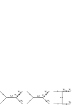
Figure 11: Contributions to $e^{+}e^{-}\rightarrow W^{+}_{P}W^{-}_{S}$ amplitudes from corrections to the external lines for unphysical scalars. The arrows on the $W$- and Goldstone-boson lines indicate the flow of negative electric charge.

We find

$${\cal M}^{{\rm[}W_{S},\chi{\rm]}}(e^{+}e^{-}\rightarrow W^{+}_{P}W^{-}_{S})$$

$$=\left\{{\cal M}(\gamma)+{\cal M}(Z)+{\cal M}(t)\right\}\Pi_{S,W_{S}}^{W_{S}W_{S}}(m_{W}^{2})+\left\{\widetilde{{\cal M}}(\gamma)+\widetilde{{\cal M}}(Z)\right\}\Pi_{S,W_{S}}^{\chi W_{S}}(m_{W}^{2})\;,$$ (B.4)

where $\Pi_{S,W_{S}}^{\phi_{1}\phi_{2}}(p^{2})$ is the propagator function for the unphysical particles $\phi_{1}$ and $\phi_{2}$ ($\phi_{i}=W_{S}$, $\chi$) which is defined by

$$\Pi_{S,W_{S}}^{\phi_{1},\phi_{2}}(p^{2})\equiv\frac{\Pi^{\phi_{1},\phi_{2}}(p^{2})-\Pi^{\phi_{1},\phi_{2}}(\xi m_{W}^{2})}{p^{2}-\xi m_{W}^{2}}\;,$$ (B.5)

where $\xi m_{W}^{2}$ is the common mass-squired of the $\phi_{i}$ scalars. Fig. 12 shows the Feynman diagrams that include corrections to the external lines for unphysical scalars and contribute to the $H_{j,\tau}^{{{\rm[}W_{S},\chi{\rm]}}}$ form factors for the $e^{+}e^{-}\rightarrow W^{+}_{P}\chi^{-}$ amplitudes.

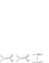
Figure 12: Contributions to $e^{+}e^{-}\rightarrow W^{+}_{P}\chi^{-}$ amplitudes from corrections to the external lines for unphysical scalars. The arrows on the $W$- and Goldstone-boson lines indicate the flow of negative electric charge.

We find

$${\cal M}^{{\rm[}W_{S},\chi{\rm]}}(e^{+}e^{-}\rightarrow W^{+}_{P}\chi^{-})$$

$$=\left\{\widetilde{{\cal M}}(\gamma)+\widetilde{{\cal M}}(Z)\right\}\Pi_{S,W_{S}}^{\chi\chi}(m_{W}^{2})+\left\{{\cal M}(\gamma)+{\cal M}(Z)+{\cal M}(t)\right\}\Pi_{S,W_{S}}^{W_{S}\chi}(m_{W}^{2})\;.$$ (B.6)

Therefore,

$${\cal M}^{{\rm[}W_{S},\chi{\rm]}}(e^{+}e^{-}\rightarrow W^{+}_{P}W^{-}_{S})+i{\cal M}^{{\rm[}W_{S},\chi{\rm]}}(e^{+}e^{-}\rightarrow W^{+}_{P}\chi^{-})$$

$$=\left\{{\cal M}(\gamma)+{\cal M}(Z)+{\cal M}(t)\right\}\left\{\Pi_{S,W_{S}}^{W_{S}W_{S}}(m_{W}^{2})+i\Pi_{S,W_{S}}^{W_{S}\chi}(m_{W}^{2})\right\}$$

$$\;\;\;\;\;\;\;\;\;\;\;\;\;\;\;\;+\left\{\widetilde{{\cal M}}(\gamma)+\widetilde{{\cal M}}(Z)\right\}\left\{\Pi_{S,W_{S}}^{\chi W_{S}}(m_{W}^{2})+i\Pi_{S,W_{S}}^{\chi\chi}(m_{W}^{2})\right\}$$

$$=\left\{{\cal M}(\gamma)+{\cal M}(Z)+{\cal M}(t)\right\}\left\{\Pi_{S,W_{S}}^{W_{S}W_{S}}(m_{W}^{2})+i\Pi_{S,W_{S}}^{W_{S}\chi}(m_{W}^{2})+i\Pi_{S,W_{S}}^{\chi W_{S}}(m_{W}^{2})-\Pi_{S,W_{S}}^{\chi\chi}(m_{W}^{2})\right\},$$

(B.7)

where we have used the tree-level identity in Eqn. (B.3). The right-hand side of Eqn. (B.7) is identically zero by the following Ward identity for the unphysical two-point functions[13]:

$$\Pi^{W_{S}W_{S}}({q^{2}})+i\,\Pi^{W_{S}\chi}({q^{2}})+i\,\Pi^{\chi W_{S}}({q^{2}})-\Pi^{\chi\chi}({q^{2}})=0\;.$$ (B.8)

Finally, by expanding the left-hand side of Eqn. (B.7) in the $\overline{S}^{\mu\beta}_{j}$ tensors we obtain Eqn. (6.6).

Appendix C One-loop vertex corrections

The propagator corrections from scalar-fermion loops were presented in Appendix A. In this section we will present the vertex corrections from the scalar fermions $(\tilde{u}_{L},\tilde{d}_{L})^{T}$, $\tilde{u}_{R}$ and $\tilde{d}_{R}$. Complete and general results for the MSSM will be presented in Ref. [16].

C.1 $WW\gamma$ and $WWZ$ vertex corrections

We begin by assigning masses and momenta as in Fig. 13.

Figure 13: Mass and momentum assignments for the calculation of the scalar-fermion triangle-type (SFT) loop corrections to $WW\gamma$ and $WWZ$ vertices. All momenta are incoming. The arrows along the $W$-boson lines indicate the flow of negative electric charge.

Note that in the definition of the tensors $T_{i}^{\mu\alpha\beta}$ of Eqns. (2.6a)-(2.6p) we used the outgoing $W$-boson momenta $p$ and $\overline{p}$. See Fig. 1. In order to be consistent with the notation of the Fortran package FF[21] and that of Ref. [17] we evaluate our loop integrals using the incoming momenta $p_{1}=-p$ and $p_{2}=-\overline{p}$.

If we neglect the coupling factors and employ arbitrary masses $m_{1}$, $m_{2}$ and $m_{3}$, then the calculation of the graph in Fig. 13, yields the following tensor structure

$$T_{\rm SFT}^{\mu\alpha\beta}(p_{1},p_{2},m_{1}^{2},m_{2}^{2},m_{3}^{2})=\sum_{i}C^{\rm SF}_{i}(p_{1},p_{2},m_{1}^{2},m_{2}^{2},m_{3}^{2})T_{i}^{\mu\alpha\beta}\;,$$ (C.1)

where the nonzero $C^{\rm SF}_{i}$ are given by

$$C^{\rm SF}_{1}(p_{1},p_{2},m_{1}^{2},m_{2}^{2},m_{3}^{2}) = 4(C_{36}-C_{35})\;,$$ (C.2a)

$$C^{\rm SF}_{2}(p_{1},p_{2},m_{1}^{2},m_{2}^{2},m_{3}^{2}) = 4m_{W}^{2}(C_{33}-C_{34}+C_{23}-C_{22})\;,$$ (C.2b)

$$C^{\rm SF}_{3}(p_{1},p_{2},m_{1}^{2},m_{2}^{2},m_{3}^{2}) = 4(C_{35}-C_{36}+C_{24})\;,$$ (C.2c)

$$C^{\rm SF}_{10}(p_{1},p_{2},m_{1}^{2},m_{2}^{2},m_{3}^{2}) = 4(2C_{36}-2C_{35}-C_{24})\;,$$ (C.2d)

$$C^{\rm SF}_{11}(p_{1},p_{2},m_{1}^{2},m_{2}^{2},m_{3}^{2}) = 2m_{W}^{2}(4C_{33}-2C_{34}-2C_{31}+5C_{23}$$ (C.2e)

$$\makebox[56.9055pt]{}-2C_{22}-3C_{21}+C_{12}-C_{11})\;,$$

$$C^{\rm SF}_{13}(p_{1},p_{2},m_{1}^{2},m_{2}^{2},m_{3}^{2}) = -C^{\rm SF}_{10}\;,$$ (C.2f)

$$C^{\rm SF}_{14}(p_{1},p_{2},m_{1}^{2},m_{2}^{2},m_{3}^{2}) = 2m_{W}^{2}(4C_{34}-2C_{33}-2C_{32}+C_{22}-C_{23})\;,$$ (C.2g)

$$C^{\rm SF}_{16}(p_{1},p_{2},m_{1}^{2},m_{2}^{2},m_{3}^{2}) = m_{W}^{2}(-12C_{34}+12C_{33}+4C_{32}-4C_{31}$$ (C.2h)

$$\makebox[56.9055pt]{}+16C_{23}-8C_{22}-8C_{21}+3C_{12}-3C_{11})\;.$$

Only the the nonvanishing $C_{i}^{\rm SF}$-functions are listed. The various $C$-functions on the right-hand side, which are discussed in Appendix E, are assigned the same arguments as the functions on the left-hand side. The next step is to provide the correct couplings and masses and then sum over all triangle graphs. For the $WW\gamma$ vertex we find,

$$f_{i}^{\gamma\,(1)\,{\rm SFT}}=\frac{N_{c}}{2}\frac{\hat{g}^{2}}{16\pi^{2}}\bigg{[}Q_{\tilde{u}}C_{i}^{\rm SF}(p_{1},p_{2},m^{2}_{\tilde{u}_{L}},m^{2}_{\tilde{d}_{L}},m^{2}_{\tilde{u}_{L}})-Q_{\tilde{d}}C_{i}^{\rm SF}(p_{1},p_{2},m^{2}_{\tilde{d}_{L}},m^{2}_{\tilde{u}_{L}},m^{2}_{\tilde{d}_{L}})\bigg{]}\;,$$ (C.3)

while the result for the $WWZ$ vertex is

$$f_{i}^{Z\,(1)\,{\rm SFT}} = \frac{N_{c}}{2}\frac{\hat{g}_{Z}^{2}}{16\pi^{2}}\bigg{[}(T^{3}_{\tilde{u}_{L}}-\hat{s}^{2}Q_{\tilde{u}})C_{i}^{\rm SF}(p_{1},p_{2},m^{2}_{\tilde{u}_{L}},m^{2}_{\tilde{d}_{L}},m^{2}_{\tilde{u}_{L}})$$ (C.4)

$$\makebox[56.9055pt]{}-(T^{3}_{\tilde{d}_{L}}-\hat{s}^{2}Q_{\tilde{d}})C_{i}^{\rm SF}(p_{1},p_{2},m^{2}_{\tilde{d}_{L}},m^{2}_{\tilde{u}_{L}},m^{2}_{\tilde{d}_{L}})\bigg{]}\;.$$

The superscript ‘SFT’ indicates the scalar-fermion triangle-type correction. The $f_{i}^{\gamma\,(1)\,{\rm SFT}}$ form factors of Eqn. (C.3) and the $f_{i}^{Z\,(1)\,{\rm SFT}}$ form factors of Eqn. (C.4) are nonvanishing whenever the corresponding $C_{i}^{\rm SF}$ functions of Eqns. (C.2a)-(C.2h) are nonvanishing.

The other type of vertex loop correction includes one scalar-fermion seagull-type (SFSG) vertex. See Fig. 14.

Figure 14: Corrections to $WW\gamma$ and $WWZ$ vertices involving one scalar-fermion seagull (SFSG) vertex. These graphs contribute only for unphysical polarizations of the $W$ bosons. The arrows along the $W$-boson lines indicate the flow of negative electric charge.

These Feynman diagrams are explicitly proportional to the momentum of the $W$ boson attached to the three-point vertex in the loop, and hence they contribute only when the same $W$-boson has an unphysical scalar polarization. An explicit calculation yields

$$f_{10}^{\gamma\,(1)\,{\rm SFSG}} = -\frac{N_{c}}{2}\frac{\hat{g}^{2}}{16\pi^{2}}(Q_{\tilde{u}}+Q_{\tilde{d}})\Big{[}2B_{1}+B_{0}\Big{]}(m_{W}^{2},m^{2}_{\tilde{d}_{L}},m^{2}_{\tilde{d}_{R}})\;,$$ (C.5a)

$$f_{13}^{\gamma\,(1)\,{\rm SFSG}} = -f_{10}^{\gamma\,(1)\,{\rm SFSG}}\;,$$ (C.5b)

for the $WW\gamma$ vertex. For the $WWZ$ vertex we find

$$f_{10}^{Z\,(1)\,{\rm SFSG}} = \frac{N_{c}}{2}\frac{\hat{g}_{Z}^{2}\hat{s}^{2}}{16\pi^{2}}(Q_{\tilde{u}}+Q_{\tilde{d}})\Big{[}2B_{1}+B_{0}\Big{]}(m_{W}^{2},m^{2}_{\tilde{d}_{L}},m^{2}_{\tilde{d}_{R}})\;,$$ (C.6a)

$$f_{13}^{Z\,(1)\,{\rm SFSG}} = -f_{10}^{Z\,(1)\,{\rm SFSG}}\;.$$ (C.6b)

Only the nonvanishing form factors are shown.

C.2 $W^{\pm}\chi^{\mp}\gamma$ and $W^{\pm}\chi^{\mp}Z$ vertex corrections

We begin by assigning masses and momenta as in Fig. 15.

Figure 15: Mass and momentum assignments for the calculation of the scalar-fermion triangle-type (SFT) one-loop contributions to $W^{\pm}\chi^{\mp}\gamma$ and $W^{\pm}\chi^{\mp}Z$ vertices. All momenta are incoming. The arrows along the $W$- and Goldstone-boson lines indicate the flow of negative electric charge.

Neglecting coupling factors and computing the loops yields the following tensor structures:

$$S^{\mu\alpha}_{\rm SFT}(p_{1},p_{2},m_{1}^{2},m_{2}^{2},m_{3}^{2}) = \sum_{i}c_{i}^{\rm SF}(p_{1},p_{2},m_{1}^{2},m_{2}^{2},m_{3}^{2})S_{i}^{\mu\alpha}\;,$$ (C.7a)

$$\overline{S}^{\mu\beta}_{\rm SFT}(p_{1},p_{2},m_{1}^{2},m_{2}^{2},m_{3}^{2}) = \sum_{i}\overline{c}_{i}^{\rm SF}(p_{1},p_{2},m_{1}^{2},m_{2}^{2},m_{3}^{2})\overline{S}_{i}^{\mu\beta}\;,$$ (C.7b)

corresponding to Fig. 15(a) and Fig. 15(b) respectively. The $c^{\rm SF}$ functions are given by

$$c_{1}^{\rm SF}(p_{1},p_{2},m_{1}^{2},m_{2}^{2},m_{3}^{2}) = 4C_{24}/m_{W}\;,$$ (C.8a)

$$c_{2}^{\rm SF}(p_{1},p_{2},m_{1}^{2},m_{2}^{2},m_{3}^{2}) = 2m_{W}(C_{22}-C_{23})\;,$$ (C.8b)

$$c_{3}^{\rm SF}(p_{1},p_{2},m_{1}^{2},m_{2}^{2},m_{3}^{2}) = 0\;,$$ (C.8c)

$$c_{4}^{\rm SF}(p_{1},p_{2},m_{1}^{2},m_{2}^{2},m_{3}^{2}) = m_{W}(2C_{21}-2C_{22}+C_{11}-C_{12})\;,$$ (C.8d)

and the $\overline{c}^{\rm SF}$ functions are

$$\overline{c}_{1}^{\rm SF}(p_{1},p_{2},m_{1}^{2},m_{2}^{2},m_{3}^{2}) = 4C_{24}/m_{W}\;,$$ (C.9a)

$$\overline{c}_{2}^{\rm SF}(p_{1},p_{2},m_{1}^{2},m_{2}^{2},m_{3}^{2}) = 2m_{W}(C_{21}-C_{23}+C_{11}-C_{12})\;,$$ (C.9b)

$$\overline{c}_{3}^{\rm SF}(p_{1},p_{2},m_{1}^{2},m_{2}^{2},m_{3}^{2}) = 0\;,$$ (C.9c)

$$\overline{c}_{4}^{\rm SF}(p_{1},p_{2},m_{1}^{2},m_{2}^{2},m_{3}^{2}) = m_{W}(2C_{21}-2C_{22}+3C_{11}-3C_{12})\;.$$ (C.9d)

In both cases the $C$-functions on the right-hand side have the same arguments as the functions on the left-hand side. It can be shown that

$$c_{i}^{\rm SF}(p_{1},p_{2},m_{1}^{2},m_{2}^{2},m_{3}^{2})=\overline{c}_{i}^{\rm SF}(p_{1},p_{2},m_{1}^{2},m_{2}^{2},m_{3}^{2})\;.$$ (C.10)

Upon incorporating the correct masses and coupling factors we obtain

$$\overline{h}_{i}^{\gamma\,(1)\,{\rm SFT}} = \frac{N_{c}}{2}\frac{\hat{g}^{2}}{16\pi^{2}}\frac{m^{2}_{\tilde{u}_{L}}-m^{2}_{\tilde{d}_{L}}}{m_{W}}\Big{[}Q_{\tilde{u}}\overline{c}_{i}^{\rm SF}(p_{1},p_{2},m^{2}_{\tilde{u}_{L}},m^{2}_{\tilde{d}_{L}},m^{2}_{\tilde{u}_{L}})$$ (C.11a)

$$\makebox[142.26378pt]{}+Q_{\tilde{d}}\overline{c}_{i}^{\rm SF}(p_{1},p_{2},m^{2}_{\tilde{d}_{L}},m^{2}_{\tilde{u}_{L}},m^{2}_{\tilde{d}_{L}})\Big{]}\;,$$

$$\overline{h}_{i}^{Z\,(1)\,{\rm SFT}} = \frac{N_{c}}{2}\frac{\hat{g}_{Z}^{2}}{16\pi^{2}}\frac{m^{2}_{\tilde{u}_{L}}-m^{2}_{\tilde{d}_{L}}}{m_{W}}\Big{[}(T^{3}_{\tilde{u}_{L}}-\hat{s}^{2}Q_{\tilde{u}})\overline{c}_{i}^{\rm SF}(p_{1},p_{2},m^{2}_{\tilde{u}_{L}},m^{2}_{\tilde{d}_{L}},m^{2}_{\tilde{u}_{L}})$$ (C.11b)

$$\makebox[142.26378pt]{}+(T^{3}_{\tilde{d}_{L}}-\hat{s}^{2}Q_{\tilde{d}})\overline{c}_{i}^{\rm SF}(p_{1},p_{2},m^{2}_{\tilde{d}_{L}},m^{2}_{\tilde{u}_{L}},m^{2}_{\tilde{d}_{L}})\Big{]}\;,$$

and

$$h_{i}^{\gamma\,(1)\,{\rm SFT}} = -\overline{h}_{i}^{\gamma\,(1)\,{\rm SFT}}\;,$$ (C.12a)

$$h_{i}^{Z\,(1)\,{\rm SFT}} = -\overline{h}_{i}^{Z\,(1)\,{\rm SFT}}\;.$$ (C.12b)

The Yukawa coupling introduces a factor of mass-dimension one while the $c_{i}^{\rm SF}$ and $\overline{c}_{i}^{\rm SF}$ functions introduce one inverse power of mass. Hence, the $h_{i}^{V\,(1)\,{\rm SFT}}$ and $\overline{h}_{i}^{V\,(1)\,{\rm SFT}}$ loop functions, $V=\gamma,Z$, are dimensionless, as expected.

There are also contributions from the loop diagrams that include a seagull vertex. See Fig. 16 for the mass and momentum assignments.

Figure 16: One-loop diagrams that contain a scalar-fermion seagull (SFSG) vertex and contribute to $W^{\pm}\chi^{\mp}\gamma$ and $W^{\pm}\chi^{\mp}Z$ vertices. The arrows along the $W$- and Goldstone-boson lines indicate the flow of negative electric charge.

By explicit calculation we find the nonzero contributions are

$$\overline{h}_{1}^{\gamma\,(1)\,{\rm SFSG}} = -\frac{N_{c}}{2}\frac{\hat{g}^{2}}{16\pi^{2}}\frac{m^{2}_{\tilde{u}_{L}}-m^{2}_{\tilde{d}_{L}}}{m_{W}^{2}}(Q_{\tilde{u}}+Q_{\tilde{d}})B_{0}(m_{W}^{2},m^{2}_{\tilde{d}_{L}},m^{2}_{\tilde{u}_{L}})\;,$$ (C.13a)

$$\overline{h}_{1}^{Z\,(1)\,{\rm SFSG}} = \frac{N_{c}}{2}\frac{\hat{g}_{Z}^{2}\hat{s}^{2}}{16\pi^{2}}\frac{m^{2}_{\tilde{u}_{L}}-m^{2}_{\tilde{d}_{L}}}{m_{W}^{2}}(Q_{\tilde{u}}+Q_{\tilde{d}})B_{0}(m_{W}^{2},m^{2}_{\tilde{d}_{L}},m^{2}_{\tilde{u}_{L}})\;,$$ (C.13b)

and

$$h_{1}^{\gamma\,(1)\,{\rm SFSG}} = -\overline{h}_{1}^{\gamma\,(1)\,{\rm SFSG}}\;,$$ (C.14a)

$$h_{1}^{Z\,(1)\,{\rm SFSG}} = -\overline{h}_{1}^{Z\,(1)\,{\rm SFSG}}\;.$$ (C.14b)

Appendix D BRS sum rules at one loop

The contributions of the vertex corrections to the BRS sum rules involve complicated algebra. Many of the details are given in this appendix. We begin with some identities involving the three-point tensor integrals. Starting from Eqn. (E.12) of Appendix E we specialize to the case $m_{1}=m_{3}$, $p_{1}^{2}=p_{2}^{2}=m_{W}^{2}$ and $(p_{1}+p_{2})^{2}=s$. We find

$$\Big{[}C_{35}-C_{36}+C_{24}\Big{]}(p_{1},p_{2},m_{1}^{2},m_{2}^{2},m_{1}^{2})=$$ (D.1a)

$$\frac{1}{s-4m_{W}^{2}}\bigg{\{}2\Big{[}B_{22}^{(12)}-B_{22}^{(13)}\Big{]}+2\big{(}m_{1}^{2}-m_{2}^{2}-m_{W}^{2}\big{)}C_{24}(p_{1},p_{2},m_{1}^{2},m_{2}^{2},m_{1}^{2})\bigg{\}}\;,$$

$$\Big{[}2C_{35}-2C_{36}+C_{24}\Big{]}(p_{1},p_{2},m_{1}^{2},m_{2}^{2},m_{1}^{2})=$$ (D.1b)

$$\frac{1}{s-4m_{W}^{2}}\bigg{\{}4\Big{[}B_{22}^{(12)}-B_{22}^{(13)}\Big{]}+\big{(}4m_{1}^{2}-4m_{2}^{2}-s\big{)}C_{24}(p_{1},p_{2},m_{1}^{2},m_{2}^{2},m_{1}^{2})\bigg{\}}\;,$$

where the shorthand notation for the $B$ functions is also given in Appendix E. Using these identities and Eqns. (C.2a)-(C.2h) we find

$$\makebox[-28.45274pt]{}\sum_{i=1}^{16}\overline{\xi}_{i1}C_{i}^{\rm SF}(p_{1},p_{2},m_{1}^{2},m_{2}^{2},m_{1}^{2}) = 2\gamma^{2}C_{3}^{\rm SF}(p_{1},p_{2},m_{1}^{2},m_{2}^{2},m_{1}^{2})+C_{10}^{\rm SF}(p_{1},p_{2},m_{1}^{2},m_{2}^{2},m_{1}^{2})$$ (D.2a)

$$= \frac{4}{m_{W}^{2}}\bigg{\{}B_{22}^{(12)}-B_{22}^{(13)}+\big{(}m_{1}^{2}-m_{2}^{2}\big{)}C_{24}(p_{1},p_{2},m_{1}^{2},m_{2}^{2},m_{1}^{2})\bigg{\}}\;.$$ (D.2b)

Incorporating Eqns. (C.3) and (C.11a) leads to

$$\makebox[-28.45274pt]{}\sum_{i=1}^{16}\overline{\xi}_{i1}f_{i}^{\gamma\,(1)\,{\rm SFT}}-\overline{h}_{1}^{\gamma\,(1)\,{\rm SFT}} = \frac{N_{c}}{2}\frac{\hat{g}^{2}}{16\pi^{2}}\frac{4}{m_{W}^{2}}\bigg{\{}Q_{\tilde{u}}\Big{[}B_{22}(m_{W}^{2},m^{2}_{\tilde{u}_{L}},m^{2}_{\tilde{d}_{L}})-B_{22}(s,m^{2}_{\tilde{u}_{L}},m^{2}_{\tilde{u}_{L}})\Big{]}$$ (D.3)

$$\makebox[71.13188pt]{}-Q_{\tilde{d}}\Big{[}B_{22}(m_{W}^{2},m^{2}_{\tilde{d}_{L}},m^{2}_{\tilde{u}_{L}})-B_{22}(s,m^{2}_{\tilde{d}_{L}},m^{2}_{\tilde{d}_{L}})\Big{]}\bigg{\}}\;,$$

while from Eqns. (C.4) and (C.11b) we obtain

$$\makebox[-28.45274pt]{}\sum_{i=1}^{16}\overline{\xi}_{i1}f_{i}^{Z\,(1)\,{\rm SFT}}-\overline{h}_{1}^{Z\,(1)\,{\rm SFT}} =$$ (D.4)

$$\makebox[-56.9055pt]{}\frac{N_{c}}{2}\frac{\hat{g}_{Z}^{2}}{16\pi^{2}}\frac{4}{m_{W}^{2}}\bigg{\{}\big{(}T^{3}_{\tilde{u}_{L}}-\hat{s}^{2}Q_{\tilde{u}}\big{)}\Big{[}B_{22}(m_{W}^{2},m^{2}_{\tilde{u}_{L}},m^{2}_{\tilde{d}_{L}})-B_{22}(s,m^{2}_{\tilde{u}_{L}},m^{2}_{\tilde{u}_{L}})\Big{]}$$

$$\makebox[5.69046pt]{}-\big{(}T^{3}_{\tilde{d}_{L}}-\hat{s}^{2}Q_{\tilde{d}}\big{)}\Big{[}B_{22}(m_{W}^{2},m^{2}_{\tilde{d}_{L}},m^{2}_{\tilde{u}_{L}})-B_{22}(s,m^{2}_{\tilde{d}_{L}},m^{2}_{\tilde{d}_{L}})\Big{]}\bigg{\}}\;.$$

The $C$ functions have completely canceled, and the result depends only on $B$ functions.

Another useful identity among loop-integral functions is

$$m_{W}^{2}\Big{[}2B_{1}+B_{0}\Big{]}(m_{W}^{2},m_{1}^{2},m_{2}^{2})=A(m_{1}^{2})-A(m_{2}^{2})-\big{(}m_{1}^{2}-m_{2}^{2}\big{)}B_{0}(m_{W}^{2},m_{1}^{2},m_{2}^{2})\;.$$ (D.5)

Using this we can show

$$\sum_{i=1}^{16}\overline{\xi}_{i1}f_{i}^{\gamma\,(1)\,{\rm SFSG}}-\overline{h}_{1}^{\gamma\,(1)\,{\rm SFSG}} = \frac{N_{c}}{2}\frac{\hat{g}^{2}}{16\pi^{2}}\frac{1}{m_{W}^{2}}(Q_{\tilde{u}}+Q_{\tilde{d}})\bigg{\{}A(m^{2}_{\tilde{u}_{L}})-A(m^{2}_{\tilde{d}_{L}})\bigg{\}}\;,$$ (D.6a)

$$\sum_{i=1}^{16}\overline{\xi}_{i1}f_{i}^{Z\,(1)\,{\rm SFSG}}-\overline{h}_{1}^{Z\,(1)\,{\rm SFSG}} = \frac{N_{c}}{2}\frac{\hat{g}_{Z}^{2}\hat{s}^{2}}{16\pi^{2}}\frac{1}{m_{W}^{2}}(Q_{\tilde{u}}+Q_{\tilde{d}})\bigg{\{}A(m^{2}_{\tilde{d}_{L}})-A(m^{2}_{\tilde{u}_{L}})\bigg{\}}\;,$$ (D.6b)

where $f_{10}^{\gamma\,(1)\,{\rm SFSG}}$ and $f_{10}^{Z\,(1)\,{\rm SFSG}}$ are the only $f_{i}^{V\,(1)\,{\rm SFSG}}$ form factors to make nonzero contributions. Combining the two types of graphs we write

$$\overline{G}_{1,\tau}^{{\rm[}\gamma{\rm,VTX]}} = -\frac{N_{c}}{2}\frac{\hat{g}^{2}}{16\pi^{2}}\frac{Q_{e}\hat{e}^{2}}{s\,m_{W}^{2}}\bigg{\{}B_{5}(m_{W}^{2},m^{2}_{\tilde{u}_{L}},m^{2}_{\tilde{d}_{L}})$$ (D.7a)

$$\makebox[28.45274pt]{}-Q_{\tilde{u}}B_{5}(s,m^{2}_{\tilde{u}_{L}},m^{2}_{\tilde{u}_{L}})+Q_{\tilde{d}}B_{5}(s,m^{2}_{\tilde{d}_{L}},m^{2}_{\tilde{d}_{L}})\bigg{\}}\;,$$

$$\overline{G}_{1,\tau}^{{\rm[}Z{\rm,VTX]}} = -\frac{N_{c}}{2}\frac{\hat{g}^{2}}{16\pi^{2}}\frac{(T^{3}_{e}-\hat{s}^{2}Q_{e})\hat{g}_{Z}^{2}}{(s-m_{W}^{2}/\hat{c}^{2})m_{W}^{2}}\bigg{\{}\hat{c}^{2}B_{5}(m_{W}^{2},m^{2}_{\tilde{u}_{L}},m^{2}_{\tilde{d}_{L}})$$ (D.7b)

$$\makebox[28.45274pt]{}-(T^{3}_{\tilde{u}_{L}}-\hat{s}^{2}Q_{\tilde{u}})B_{5}(s,m^{2}_{\tilde{u}_{L}},m^{2}_{\tilde{u}_{L}})+(T^{3}_{\tilde{d}_{L}}-\hat{s}^{2}Q_{\tilde{d}})B_{5}(s,m^{2}_{\tilde{d}_{L}},m^{2}_{\tilde{d}_{L}})\bigg{\}}\;,$$

where the $B_{5}$ function is defined in Eqn. (A.3). The next step is to insert factors of $2T^{3}_{\tilde{u}_{L}}=1$ and $-2T^{3}_{\tilde{d}_{L}}=1$ in appropriate places, and then we can immediately recognize the two-point functions in the basis of current eigenstates as given in Eqn. (A.4a)-(A.4d). Using the $\Pi_{T}$ functions of Appendix A we find

$$\overline{G}_{1,\tau}^{{\rm[}\gamma{\rm,VTX]}} = \frac{Q_{e}\hat{e}^{2}}{s}\frac{\hat{g}^{2}}{m_{W}^{2}}\bigg{\{}-\Pi^{11}_{T}(m_{W}^{2})+\Pi^{3Q}_{T}(s)\bigg{\}}$$ (D.8a)

$$= \frac{Q_{e}\hat{e}^{2}}{sm_{W}^{2}}\bigg{\{}-\Pi_{T}^{WW}(m_{W}^{2})+\Pi_{T}^{\gamma\gamma}(s)+\frac{\hat{c}}{\hat{s}}\Pi_{T}^{\gamma Z}(s)\bigg{\}}\;,$$

$$\overline{G}_{1,\tau}^{{\rm[}Z{\rm,VTX]}} = \frac{(T^{3}_{e}-\hat{s}^{2}Q_{e})\hat{g}_{Z}^{2}}{s-m_{W}^{2}/\hat{c}^{2}}\frac{\hat{g}^{2}}{m_{W}^{2}}\bigg{\{}-\hat{c}^{2}\Pi^{11}_{T}(m_{W}^{2})-\hat{s}^{2}\Pi^{3Q}_{T}(s)+\Pi^{33}_{T}(s)\bigg{\}}$$ (D.8b)

$$= \frac{(T^{3}_{e}-\hat{s}^{2}Q_{e})\hat{g}^{2}}{(s-m_{W}^{2}/\hat{c}^{2})m_{W}^{2}}\bigg{\{}-\Pi_{T}^{WW}(m_{W}^{2})+\Pi_{T}^{ZZ}(s)+\frac{\hat{s}}{\hat{c}}\Pi_{T}^{\gamma Z}(s)\bigg{\}}\;.$$

The contributions of all the vertex corrections to the BRS sum rules are now expressed entirely in terms of the gauge-boson propagator corrections.

Appendix E The decomposition of $C^{\mu\nu\rho}$, a rank-three three-point tensor integral

For our loop integrals we follow the notation of [17, 21]. While the tensor reduction of the three-point integrals ($C$-functions) through rank two is presented in Appendix D of Ref. [17], it is necessary to present here the reduction of the rank-three $C$-function. In order to make this appendix reasonably self-contained, we also give a brief review of the lower $C$-functions and the two-point integrals ($B$-functions).

Our measure in $D=4-2\epsilon$ dimensions, defined as

$$\overline{d^{D}k}=\Gamma(1-\epsilon)(\pi\mu^{2})^{\epsilon}d^{D}k\;,$$ (E.1)

is the $\overline{\rm MS}$ regularization[19]. Propagator factors are defined as

$$N_{1} = k^{2}-m_{1}^{2}+i\epsilon\;,$$ (E.2a)

$$N_{2} = (k+p_{1})^{2}-m_{2}^{2}+i\epsilon\;,$$ (E.2b)

$$N_{3} = (k+p_{1}+p_{2})^{2}-m_{3}^{2}+i\epsilon\;,$$ (E.2c)

and it is convenient to introduce the following short-hand notation:

$$f_{1} = m_{2}^{2}-m_{1}^{2}-p_{1}^{2}\;,$$ (E.3a)

$$f_{2} = m_{3}^{2}-m_{2}^{2}-(p_{1}+p_{2})^{2}+p_{1}^{2}\;.$$ (E.3b)

The $B$-functions are given by

$$\{B_{0},\,B^{\mu},\,B^{\mu\nu}\}(p_{1},m_{1},m_{2})=\int\frac{\overline{d^{d}k}}{i\pi^{2}}\frac{\{1,\,k^{\mu},\,k^{\mu}k^{\nu}\}}{N_{1}N_{2}}\;,$$ (E.4)

with the decompositions

$$B^{\mu}(p_{1},m_{1},m_{2}) = p_{1}^{\mu}B_{1}(p_{1},m_{1},m_{2})\;,$$ (E.5a)

$$B^{\mu\nu}(p_{1},m_{1},m_{2}) = g^{\mu\nu}B_{22}(p_{1},m_{1},m_{2})+p_{1}^{\mu}p_{1}^{\nu}B_{21}(p_{1},m_{1},m_{2})\;.$$ (E.5b)

The integrals $B_{22}$, $B_{21}$ and $B_{1}$ may be reexpressed in terms of the $B_{0}$ function and the one-point integral, $A$[11, 17]. Before proceeding it is convenient to introduce some short-hand notation that will be useful in the reductions of the $C$-functions.

$$B_{n}^{(12)} = B_{n}=B_{n}(p_{1},m_{1},m_{2})\;,$$ (E.6a)

$$B_{n}^{(13)} = B_{n}(p_{1}+p_{2},m_{1},m_{3})\;,$$ (E.6b)

$$B_{n}^{(23)} = B_{n}(p_{2},m_{2},m_{3})\;.$$ (E.6c)

where $B_{n}=B_{22}$, $B_{21}$, $B_{1}$ or $B_{0}$.

We introduce our $C$-functions by

$$\{C_{0},\,C^{\mu},\,C^{\mu\nu},\,C^{\mu\nu\rho}\}(p_{1},p_{2},m_{1},m_{2},m_{3})=\int\frac{\overline{d^{d}k}}{i\pi^{2}}\frac{\{1,\,k^{\mu},\,k^{\mu}k^{\nu},\,k^{\mu}k^{\nu}k^{\rho}\}}{N_{1}N_{2}N_{3}}\;,$$ (E.7)

and the tensor integrals may be expanded as

$$C^{\mu}(p_{1},p_{2},m_{1},m_{2},m_{3}) = p_{1}^{\mu}C_{11}+p_{2}^{\mu}C_{12}\;,$$ (E.8a)

$$C^{\mu\nu}(p_{1},p_{2},m_{1},m_{2},m_{3}) = p_{1}^{\mu}p_{1}^{\nu}C_{21}+p_{2}^{\mu}p_{2}^{\nu}C_{22}+(p_{1}^{\mu}p_{2}^{\nu}+p_{2}^{\mu}p_{1}^{\nu})C_{23}+g^{\mu\nu}C_{24}\;,$$ (E.8b)

$$C^{\mu\nu\rho}(p_{1},p_{2},m_{1},m_{2},m_{3}) = p_{1}^{\mu}p_{1}^{\nu}p_{1}^{\rho}C_{31}+p_{2}^{\mu}p_{2}^{\nu}p_{2}^{\rho}C_{32}$$ (E.8c)

$$\mbox{}+(p_{1}^{\mu}p_{1}^{\nu}p_{2}^{\rho}+p_{1}^{\mu}p_{2}^{\nu}p_{1}^{\rho}+p_{2}^{\mu}p_{1}^{\nu}p_{1}^{\rho})C_{33}+(p_{2}^{\mu}p_{2}^{\nu}p_{1}^{\rho}+p_{2}^{\mu}p_{1}^{\nu}p_{2}^{\rho}+p_{1}^{\mu}p_{2}^{\nu}p_{2}^{\rho})C_{34}$$

$$\mbox{}+(g^{\mu\nu}p_{1}^{\rho}+g^{\mu\rho}p_{1}^{\nu}+g^{\nu\rho}p_{1}^{\mu})C_{35}+(g^{\mu\nu}p_{2}^{\rho}+g^{\mu\rho}p_{2}^{\nu}+g^{\nu\rho}p_{2}^{\mu})C_{36}\;.$$

It is convenient to introduce the following $2\times 2$ matrix:

$$X=\left(\begin{array}[]{cc}2p_{1}^{2}&2p_{1}\cdot p_{2}\\ 2p_{1}\cdot p_{2}&2p_{2}^{2}\end{array}\right)$$ (E.9)

Then the reduction of the $C_{1n}$ functions is accomplished by

$$\left(\begin{array}[]{c}C_{11}\\ C_{12}\end{array}\right)=X^{-1}\left(\begin{array}[]{l}B_{0}^{(13)}-B_{0}^{(23)}+f_{1}C_{0}\\ B_{0}^{(12)}-B_{0}^{(13)}+f_{2}C_{0}\end{array}\right)\;.$$ (E.10)

For the $C_{2n}$ functions,

$$C_{24} = \frac{1}{4}+\frac{1}{4}B_{0}^{(23)}+\frac{1}{2}m_{1}^{2}C_{0}-\frac{1}{4}(f_{1}C_{11}+f_{2}C_{12})\;,$$ (E.11a)

$$\left(\begin{array}[]{c}C_{21}\\ C_{23}\end{array}\right) = X^{-1}\left(\begin{array}[]{l}B_{1}^{(13)}+B_{0}^{(23)}+f_{1}C_{11}-2C_{24}\\ B_{1}^{(12)}-B_{1}^{(13)}+f_{2}C_{11}\end{array}\right)\;,$$ (E.11f)

$$\left(\begin{array}[]{c}C_{23}\\ C_{22}\end{array}\right) = X^{-1}\left(\begin{array}[]{l}B_{1}^{(13)}-B_{1}^{(23)}+f_{1}C_{12}\\ \makebox[28.45274pt]{}-B_{1}^{(13)}+f_{2}C_{12}-2C_{24}\end{array}\right)\;.$$ (E.11k)

Finally, for the $C_{3n}$ functions,

$$\left(\begin{array}[]{c}C_{35}\\ C_{36}\end{array}\right) = X^{-1}\left(\begin{array}[]{l}B_{22}^{(13)}-B_{22}^{(23)}+f_{1}C_{24}\\ B_{22}^{(12)}-B_{22}^{(13)}+f_{2}C_{24}\end{array}\right)\;,$$ (E.12e)

$$\left(\begin{array}[]{c}C_{31}\\ C_{33}\end{array}\right) = X^{-1}\left(\begin{array}[]{l}B_{21}^{(13)}-B_{0}^{(23)}+f_{1}C_{21}-4C_{35}\\ B_{21}^{(12)}-B_{21}^{(13)}+f_{2}C_{21}\end{array}\right)\;,$$ (E.12j)

$$\left(\begin{array}[]{c}C_{34}\\ C_{32}\end{array}\right) = X^{-1}\left(\begin{array}[]{l}B_{21}^{(13)}-B_{21}^{(23)}+f_{1}C_{22}\\ \makebox[28.45274pt]{}-B_{21}^{(13)}+f_{2}C_{22}-4C_{36}\end{array}\right)\;,$$ (E.12o)

$$\left(\begin{array}[]{c}C_{33}\\ C_{34}\end{array}\right) = X^{-1}\left(\begin{array}[]{l}B_{21}^{(13)}+B_{1}^{(23)}+f_{1}C_{23}-2C_{36}\\ \makebox[28.45274pt]{}-B_{21}^{(13)}+f_{2}C_{23}-2C_{35}\end{array}\right)\;.$$ (E.12t)

It is also possible to solve for $C_{35}$ and $C_{36}$ via

$$C_{35} = -\frac{1}{9}-\frac{1}{6}B_{0}^{(23)}+\frac{1}{3}m_{1}^{2}C_{11}-\frac{1}{6}(f_{1}C_{21}+f_{2}C_{23})\;,$$ (E.13a)

$$C_{36} = -\frac{1}{18}+\frac{1}{6}B_{1}^{(23)}+\frac{1}{3}m_{1}^{2}C_{12}-\frac{1}{6}(f_{1}C_{23}+f_{2}C_{22})\;.$$ (E.13b)

These reductions can sometimes be numerically unstable, especially when the matrix of Eqn. (E.9) becomes singular. Using the equations above we are able to calculate $C_{33}$, $C_{34}$, $C_{35}$ and $C_{36}$ in two different ways. The redundancy provides a useful check of numerical reliability.

References

- [1] C. Becchi, A. Rouet and B. Stora, Commun. Math. Phys. 42 (1975); Ann. Phys. (N.Y.) 98 (1976) 287.
- [2] G.J. Gounaris, R. Kögerler and H. Neufeld, Phys. Rev. D34 (1986) 3257.
- [3] K. Hagiwara, T. Hatsukano, S. Ishihara and R. Szalapski, Nucl. Phys. B496 (1997) 66.
- [4] H. Murayama, I. Watanabe and K. Hagiwara, HELAS: HELicity Amplitude Subroutines for Feynman diagram evaluations, KEK-91-11, Jan. 1992, 184.
- [5] T. Stelzer and W.F. Long, Comput. Phys. Commun. 81 (1994) 357-371.
- [6] K. Hagiwara, H. Iwasaki, A. Miyamoto, H. Murayama and D. Zeppenfeld, Nucl. Phys. B365 (1991) 544.
- [7] C. Ann, M.E. Peskin, B.W. Lynn and S. Selipsky, Nucl. Phys. B309 (1988) 221.
- [8] J.M. Cornwall, D.N. Levin and G.Tiktopoulos, Phys. Rev. Lett. 30 (1973) 1268; Phys. Rev. D10 (1974) 1145; B.W. Lee, C. Quigg and H.B. Thacker, Phys. Rev. D16 (1977) 1519.
- [9] M.S. Chanowitz and M.K. Gaillard, Nucl. Phys. B261 (1985) 379; H. Veltman, Phys. Rev. D41 (1990) 2294.
- [10] J. Bagger and C. Schmidt, Phys. Rev. D41 (1990) 264; H.-J. He, Y.-P. Kuang and X. Li, Phys. Rev. Lett. 69 (1992) 2619; Phys. Rev. D49 (1994) 4842.
- [11] G. Passarino and M. Veltman, Nucl. Phys. B160 (1979) 151.
- [12] K. Hagiwara, S. Ishihara, R. Szalapski and D. Zeppenfeld, Phys. Rev. D48 (1993) 2182.
- [13] M. Lemoine and M. Veltman, Nucl. Phys. B164 (1980) 445.
- [14] F. Feruglio and S. Rigolin, Phys. Lett. B397 (1997) 245-254.
- [15] K. Hagiwara, R.D. Peccei, D. Zeppenfeld and K. Hikasa, Nucl. Phys. B282 (1987) 253.
- [16] S. Alam, G.C. Cho, K. Hagiwara, S. Kanemura, R. Szalapski and Y. Umeda, in preparation.
- [17] K. Hagiwara, D. Haidt, C. S. Kim and S. Matsumoto, Z. Phys. C64 (1994) 559.
- [18] S. Kanemura, KEK-Preprint 97-160 (hep-ph 9710237).
- [19] O.V. Tarasov, A.A. Vladimirov and A.Yu Zharkov, Phys. Lett. 93B (1980) 429; K.G. Chetyrkin, A.L. Kataev and F.V. Tkachov, Nucl. Phys. B174 (1987) 125.
- [20] S. Alam, Phys. Rev. D50 (1994) 124; ibid. 148; ibid. 174.
- [21] G.J. van Oldenborgh, Comput. Phys. Commun. 66 (1991) 1.