Abstract

We discuss the formulation of ”thermal renormalization group-equations” and their application to the finite temperature phase-transition of scalar $O(N)$-theories. Thermal renormalization group-equations allow for a computation of both the universal and the non-universal aspects of the critical behavior directly in terms of the zero-temperature physical couplings. They provide a nonperturbative method for a computation of quantities like real-time correlation functions in a thermal environment, where in many situations straightforward perturbation theory fails due to the bad infrared-behavior of the thermal fluctuations. We present results for the critical temperature, critical exponents and amplitudes as well as the scaling equation of state for self-interacting scalar theories.

PACS-No: 11.10.Wx, 11.15.Tk, 05.70.Fh, 05.70.Ce
Keywords: Finite temperature, Nonperturbative techniques, Critical phenomena, Thermal renormalization group

1 Introduction

In recent years, the study of field theories in a thermal environment has become increasingly popular [1]. The interest in this field has increased for a number of reasons. From the experimental side, the study of strong interactions at high temperatures and densities has been taken up by means of heavy-ion collisions. In order to understand theoretically the outcome of such experiments, we have to learn how to treat field theory in a hot and dense environment. Thermal field theory also plays an important rôle in astro-particle physics. Questions concerning the physics of the very early universe can usually only be addressed if the impact of the temperatures on the properties of matter is taken into account. A famous and in recent years extensively discussed question concerns the phase-transition that might have been associated with the restoration of the electroweak symmetry at temperatures of the order of $100$ GeV. Another interesting phase-transition is the transition from the quark-gluon plasma phase of quantum-chromodynamics to the low energy phase where confinement applies and the (approximate) chiral symmetry of the standard model is broken. This transition has taken place at temperatures of the order of $100$ MeV and is expected to be experimentally accessible with the next generation of heavy-ion colliders. It is also an interesting open question of particle physics applied to astronomy whether a quark-gluon plasma is realized in the interior of neutron stars.

A large number of open problems is connected to non-equilibrium phenomena. In the physics of the early universe this concerns for example the question of reheating after a (hypothetical) inflationary phase. Also heavy-ion collisions may not yield a thermalized state and one should strictly speaking consider QCD out of thermal equilibrium. Finally it is of interest to study the dynamics of phase-transitions in various contexts.

In marked contrast to the number of situations in which thermal (or more general non-equilibrium) field theory is of relevance is the number of open fundamental questions. This is due to the fact that in many situations even in the simpler equilibrium case the well established methods of perturbation theory fail due to a modified infrared-behavior of the theory. Famous examples of the infrared problems are the observation of Linde [3], that the free energy of a non-abelian gauge-theory is not computable in perturbation theory beyond three-loop order (irrespective of the size of the coupling constant) or the fact that even super-daisy resummed one-loop perturbation theory fails to predict the correct critical behavior of self-interacting scalar theories even if they are weakly coupled at vanishing temperature [4]. Although the physical mechanisms behind the above-mentioned problems are quite different, both problems may be traced back to the fact that the behavior of bulk-observables like the free energy or of theories close to a second order phase-transition is governed by three-dimensional physics (if the underlying zero-temperature theory is formulated in 3+1 dimensions).

We then have to devise methods that are able to cope with this effective change of the relevant degrees of freedom. One such method in principle is lattice field theory, which may be used to study time-independent quantities like the free energy also at non-vanishing temperature. Lattice studies of field theory at high temperature are however often complicated by the existence of widely separated scales and there is as yet no formulation of lattice field theory that can deal with finite density or time-dependent quantities.

Another way of dealing with theories where the relevant degrees of freedom are scale-dependent is provided by the renormalization group (RG). This is a well known fact in statistical physics, where the Wilsonian form of the renormalization group [5] is widely used in the study of critical phenomena. In the context of field theory, there are different implementations of the general RG idea. These range from the “environmentally friendly” RG ([6] and references therein) which is a variant of the Callen-Szymanzik RG, via the “auxiliary mass method” [7] to continuum implementations of the Wilsonian approach, initiated in a field-theory context by Polchinski and others [8]. This approach has in recent years been applied to a number of problems in field theory both at vanishing and non-vanishing temperature and is now also known under the name “Exact renormalization group (ERG)”-approach. The ERG-approach is a nonperturbative formulation of field theory and by construction avoids any infrared-problems irrespective of the dimensionality of the system under study. It is formulated in Euclidean space and may be straightforwardly adapted to study thermal field theory in the “imaginary-time”- or Matsubara formalism.

Recently, an implementation of the Wilsonian renormalization group in the real-time formulation of thermal field theory has been proposed [9]. This “thermal renormalization group” (TRG) has a number of advantages as compared to the ERG applied to thermal field theory. Even though the formulations of field theory in the imaginary- and the real-time formalism are in principle equivalent and one can compute any quantity of interest in both approaches, in practice recovering Green-functions at real time arguments from their expressions at discrete imaginary energies through analytical continuation is often tedious. Moreover, in practical applications of the Wilsonian RG results will usually be obtained numerically, making analytical continuation impossible. Thus, in order to study quantities like damping rates and the like [10], a real-time formulation of thermal field theory is mandatory.

Also, in the real-time formalism there is a clear separation between “thermal” and “quantum” fluctuations. The thermal renormalization group only treats the thermal fluctuations of the theory, all quantum fluctuations are assumed to be integrated out, i.e. one starts with the full physical effective action of the theory at vanishing temperature. This feature essentially prevents us from studying theories that are strongly interacting already at $T=0$ and may thus seem like a major shortcoming. On the other hand, in situations where the zero-temperature theory is weakly coupled this apparent shortcoming turns into an advantage. In such a situation the calculation of non-universal quantities such as critical temperatures in terms of the measurable couplings of the theory in the framework of the ERG requires a two step procedure, where one first has to relate physical quantities at zero temperature to the parameters of the action. These parameters are renormalization scheme dependent and one has to perform perturbative calculations using the ERG-formulation [11]. In situations where two-loop accuracy is required to fix the ambiguities of such a calculation, this procedure is highly nontrivial and has up to now only been performed in simple models [12].

Another advantage of a formulation of RG-equations only for the thermal modes is the fact that this can be done while respecting manifest gauge-invariance [13]. The general formulation of Wilsonian RG-equations relies on a separation of “hard” and “soft” modes by means of an external scale which acts as a momentum cutoff. This procedure is in general not consistent with gauge-invariance (see however [15] for a different approach circumventing this problem), and one obtains generalized Slavnov-Taylor identities that may be interpreted as fine-tuning conditions that have to be respected in order to regain BRS-invariance of the physical effective action [16]. In the framework of the TRG one avoids this problem since only the physical fields have thermal fluctuations. Manifest gauge-invariance severely restricts the form of possible contributions to the effective action and thus helps in making sensible approximations (see the discussion below).

In the present paper we present an extensive application of the TRG to the critical behavior of the simplest nontrivial field-theories in $3+1$ dimensions, scalar self-interacting models with a (at zero temperature spontaneously broken) $O(N)$-symmetry. Despite their simplicity, already these theories are not accessible in straightforward perturbation theory for temperatures close to the critical one. $O(N)$-symmetric scalar theories have a number of applications both in the context of statistical physics and in particle physics. In statistical physics, these models are used for example for the description of polymers (in the limit $N=0$), the liquid-vapor transition ($N=1$, the Ising model), the transition of helium to a superfluid state ($N=2$) or ferromagnetic systems (the Heisenberg model, $N=3$). In particle physics, the model with $N=4$ at zero temperature describes the scalar part of the Lagrangian of the standard model. At non-vanishing temperature the theory with one scalar field shows the same universal behavior as the standard model for the critical value of the zero-temperature Higgs mass [17]. For $N=4$ the universal behavior should be the same as that of the chiral phase-transition in the $N_{f}=2$ chiral limit of QCD.

The universal behavior of the theory may be studied directly in three dimensions. There are accurate results on critical exponents from methods like (Borel-resummed) $\epsilon$-expansion, from perturbative calculation at fixed dimension, from resummed high-temperature series or from lattice studies (for a review, see [18]). There are also a number of studies using the ERG directly in three dimensions (for example [19, 20, 21]). Also the scaling equation of state (EOS) has been widely studied in the three-dimensional theory ([20]-[24], see also [18]).

On the other hand, the number of studies of the full $3+1$-dimensional theory at finite temperature close to the phase-transition is rather limited. Results on the critical temperature and exponents in the ERG-approach are given in [25]-[28], and for $N=1$ $T_{c}$, exponents and critical amplitude ratios have been studied by means of the environmentally friendly RG in [29]. The critical temperature and some exponents have also been obtained through the auxiliary mass method in [30]. Results for critical exponents from the TRG have been given for $N=1$ in [9] and critical exponents as well as the equation of state for $N=1$ have been obtained from the TRG in [31]. We here extend these studies to arbitrary $N$ and furthermore give critical temperatures, the scaling form of the equation of state as well as critical amplitudes in terms of the zero-temperature couplings for the cases $N=1$ and $N=4$. For reasons to be discussed below our results on the universal critical behavior are not as accurate as the existing results obtained in the effective three-dimensional theory. On the other hand, the present work does not rely on universality arguments and the approximations made in the present paper may be improved. The TRG allows for the direct computation also of real-time quantities and offers a convenient nonperturbative tool to study field theory in a hot and – after a straightforward extension of the method possibly dense – environment.

The format of the paper is as follows: In the next section we give a review of the formulation of the thermal renormalization group-equation and discuss some general points regarding the possibilities of approximately solving equations of this general type. Here we can rely on experience gained from the study of the Euclidean exact renormalization group-equation. In section 3 we apply the method to $O(N)$-symmetric scalar theories. After deriving the flow-equation for the effective potential we discuss in detail the phase-transition for $N=1$ and $N=4$. We compare our results for the critical temperatures, critical exponents and amplitudes and the scaling equation of state with different results given in the literature. We also discuss the dependence of the critical temperature on the number of fields and compare with the expectations from large-$N$ and naive perturbation theory.

Section 4 contains our concluding remarks.

2 The Thermal Renormalization Group-equation

In this section we discuss the derivation of the thermal renormalization group (TRG)-equation [9] and some more general points on its relevance and strategies for its approximate solution.

The basic objective of thermal renormalization group-equations in the framework proposed in [9] is to use the Wilsonian RG-approach in the real-time formulation of thermal field theory in order to have access to real-time correlation functions avoiding the need for analytical continuation. Wilsonian renormalization group-equations are generally not very useful in Minkowski-space, since the connection between $k^{2}$ and ”softness” of modes is lost. On the other hand, in many situations the problematic behavior of perturbation theory at finite temperature is only due to the thermal modes, and the dynamics of the theory in the vicinity of a phase-transition is governed by three-dimensional classical statistics. To deal with this particular problem, one may use the fact that in real-time the propagators clearly discriminate between ”thermal” and ”quantum” fluctuations to treat the thermal contributions with renormalization group methods, leaving the quantum contributions untouched.

2.1 Formulation of the TRG-equation

Field-theory, not necessarily in a thermal equilibrium situation, may be formulated using the Schwinger-Keldysh or closed time-path (CTP) formulation [32]. Here one is interested in expectation-values of operators with respect to some general density-matrix rather than in scattering amplitudes, i.e. matrix-elements of the form $\langle{\mbox{out}}|{\mbox{in}}\rangle$ as in the more conventional approach to field-theory at vanishing temperature. In the CTP-formalism one thus considers matrix elements of the form $\langle{\mbox{in}}|{\mbox{in}}\rangle$. In order to be able to derive correlation-functions at different times, one defines the generating functional $Z$ which should now depend on two sources (in the case of one real field) $J_{1}$ and $J_{2}$ by inserting a complete set of states at some time $t$ as

$$Z[J_{1},J_{2}] = \int\delta\Phi\langle{\mbox{in}},t_{0}|\Phi,t\rangle_{J_{2}}\langle\Phi,t|{\mbox{in}},t_{0}\rangle_{J_{1}}$$ (1)

where all states are in the Heisenberg picture and $Z$ of course depends on the initial state of the system. One may as usually introduce the path-integral representation for the transition matrix elements $\langle{\mbox{in}},t_{0}|\Phi,t\rangle_{J_{i}}$ to find

$$Z[J_{1},J_{2}] = \int\delta\Phi\langle{\mbox{in}},t_{0}|T^{*}\exp\left(-i\int_{t_{0}}^{t}d\bar{t}d^{3}xJ_{2}\phi_{H}\right)|\Phi,t\rangle\times$$ (2)

$$\qquad\quad\times\langle\Phi,t|T\exp\left(i\int_{t_{0}}^{t}d\bar{t}d^{3}xJ_{1}\phi_{H}\right)|{\mbox{in}},t_{0}\rangle$$

where $T$ and $T^{*}$ represent the time- and the anti-time-ordering operator respectively and $\phi_{H}$ are Heisenberg-fields. Note that the sources $J_{1}$ and $J_{2}$ have to be different in order to obtain time-dependent correlation functions.

Finally, one may also formulate the generating functional by introducing the density matrix $\rho$ that characterizes the initial state. The generating functional then simply is the ensemble-average of the product of the time- and anti-time-ordered exponentials and we can write

$$Z[J_{1},J_{2},\rho] = N{\mbox{ Tr}}\biggl{\{}\rho\left[T^{*}\exp\left(-i\int_{t_{0}}^{t}d\bar{t}d^{3}xJ_{2}\phi_{H}\right)\right]\times$$ (3)

$$\qquad\times\left[T\exp\left(i\int_{t_{0}}^{t}d\bar{t}d^{3}xJ_{1}\phi_{H}\right)\right]\biggr{\}}$$

$$= \int\delta\phi\delta\phi^{\prime}\delta\Phi\langle\phi,t_{0}|\rho|\phi^{\prime},t_{0}\rangle\langle\phi^{\prime},t_{0}|T^{*}\exp\left(-i\int_{t_{0}}^{t}d\bar{t}d^{3}xJ_{2}\phi_{H}\right)|\Phi,t\rangle\times$$

$$\qquad\quad\times\langle\Phi,t|T\exp\left(i\int_{t_{0}}^{t}d\bar{t}d^{3}xJ_{1}\phi_{H},t_{0}\right)|\phi,t_{0}\rangle$$

Derivatives of $Z$ with respect to the sources thus generate ensemble-averages (expectation values) of products of Heisenberg-fields. Due to the introduction of the two independent sources and the fact that we are computing matrix-elements between ”in”-states at equal time, while inserting a complete set of states at a different time $t$ and using time- and anti-time-ordered exponentials the integration-contour is a closed path from $t_{0}$ to $t$ and back, thus giving rise to the name ”closed-time-path” formulation (figure 1).

Figure 1: The Schwinger-Keldysh contour in the complex time-plane. The lower part of the contour is infinitesimally shifted below the real axis.

Finally we go over to a path-integral representation of the transition elements and write

$$Z[J_{1},J_{2},\rho] = \int\delta\phi_{1}\delta\phi_{2}\langle\phi_{1},t_{0}|\rho|\phi_{2},t_{0}\rangle\exp\left[i\left(S[\phi_{1}]-S^{*}[\phi_{2}]+J_{1}\phi_{1}-J_{2}\phi_{2}\right)\right]$$ (4)

Up to now, the initial state is completely unspecified. Indeed, the matrix element $\langle\phi_{1}|\rho|\phi_{2}\rangle$ will be some functional of the configurations $\phi_{i}(\vec{x},\bar{t}=t_{0})$ which may be written as

$$\langle\phi_{1},t_{0}|\rho|\phi_{2},t_{0}\rangle = \exp\left(iK[\phi_{1},\phi_{2}]\right)$$ (5)

$$= \exp\left[i\left(K+\int d^{3}kK^{a}\phi_{a}+\frac{1}{2}\int d^{3}kd^{3}pK^{ab}\phi_{a}\phi_{b}+\ldots\right)\right]$$

where we use a compact notation with $a,b=1,2$ and metric $c_{ab}={\mbox{diag}}(+1,-1)$. We may then treat the coefficients $K^{ab...}$ as sources for the corresponding composite operators and write the generating functional as

$$Z[J^{a},K,K^{a},K^{ab},...]\!=\!\!\int\!\!\delta\phi_{1}\delta\phi_{2}\exp\left[i\left(S[\phi_{1}]\!-\!S^{*}[\phi_{2}]\!+\!J^{a}\phi_{a}\!+\!K\!+\!K^{a}\phi_{a}\!+\!\frac{1}{2}K^{ab}\phi_{a}\phi_{b}\!+...\right)\right]$$ (6)

Having specified the density matrix, i.e. the sources $K^{ab...}$, one may then proceed along the lines of [33] in order to obtain e.g. a perturbative series etc.

We will in the present paper be interested in systems with a density matrix of the general form

$$\rho_{f}=C\exp\left(-\int\frac{d^{3}k}{(2\pi)^{3}2\omega_{k}}f(|\vec{k}|)a^{\dagger}_{k}a_{k}\right)$$ (7)

where $a^{\dagger}$ and $a$ are creation- and annihilation-operators of a free scalar field respectively. (7) is a slight generalization of the corresponding thermal density-matrix which obtains for $f(|\vec{k}|)=\beta\omega_{k}$ (we may interpret (7) as the density-matrix of a system in which each mode of the field is at a different temperature given by $T_{k}=\frac{\omega_{k}}{f(|\vec{k}|)}$ — we will come back to this interpretation below). For the above density-matrix the matrix-elements of $\langle\phi_{1}|\rho|\phi_{2}\rangle$ are given by [34]

$$\langle\phi_{1}|\rho_{f}|\phi_{2}\rangle = C\exp\biggl{\{}-\frac{1}{2}\int\frac{d^{3}k}{(2\pi)^{3}}\frac{\omega_{k}}{\sinh f(|\vec{k}|)}\left[\left(\phi_{1}^{2}+\phi_{2}^{2}\right)\cosh f(|\vec{k}|)-2\phi_{1}\phi_{2}\right]\biggr{\}}$$ (8)

We observe that $K^{a}$ as well as $K^{abc}$ and all higher derivatives of $K[\phi]$ vanish in this case. The constant is absorbed in the normalization of the generating functional. The fact that only terms quadratic in $\phi_{a}$ appear in the density-matrix element is of course the reason why in finite temperature field-theory in equilibrium only the two-point functions are modified. Indeed, noting that $K^{ab}$ only has support at $t=t_{0}$, we may absorb the effects of the initial state into the boundary-conditions for the free field-equations, where they simply modify the two-point functions, yielding in the case of a thermal initial state the well-known real-time propagators of the CTP-formalism at finite temperature.

Above we have made use of the path-integral approach to the CTP-formalism. In simple theories, a convenient way to obtain explicit expressions for the propagators is through the operator-formulation. To this end, introduce a generalization of the $\Theta$-function with real time-arguments to a $\Theta$-function on the contour $C$ corresponding to eq. (3) and evaluate the path-ordered product ($T_{c}$ here is the path-ordering operator)

$$G_{f}^{(c)}(x,x^{\prime}) = \langle T_{c}\phi(x)\phi(x^{\prime})\rangle_{f}$$ (9)

$$= \Theta_{c}(t-t^{\prime})\langle\phi(x)\phi(x^{\prime})\rangle_{f}+\Theta_{c}(t^{\prime}-t)\langle\phi(x^{\prime})\phi(x)\rangle_{f}$$

after substituting for the field operators

$$\phi(x)=\int\frac{d^{3}k}{(2\pi)^{3}2\omega_{k}}\left(a_{k}e^{-ikx}+a^{\dagger}_{k}e^{ikx}\right)$$ (10)

In (9), the averages are ensemble-averages with respect to the density-matrix defined in (7) and in the usual manner one obtains, using

$$\langle a^{\dagger}_{k}a_{p}\rangle_{f} = (2\pi)^{3}2\omega_{k}\frac{1}{e^{f(|\vec{k}|)}-1}\delta(\vec{k}-\vec{p})$$

$$\langle a_{k}a^{\dagger}_{p}\rangle_{f} = (2\pi)^{3}2\omega_{k}\left(1+\frac{1}{e^{f(|\vec{k}|)}-1}\right)\delta(\vec{k}-\vec{p})$$ (11)

(note that these expressions again reduce to the well-known results for $f(|\vec{k}|)=\beta\omega_{k}$),

$$G_{f}^{(c)}(x-x^{\prime}) = iD_{f}^{(c)}(x-x^{\prime})=\int\frac{d^{4}k}{(2\pi)^{4}}2\pi\delta(k^{2}-m^{2})e^{-ik(x-x^{\prime})}\times$$ (12)

$$\qquad\quad\times\left[\Theta(k_{0})\Theta_{c}(t-t^{\prime})+\Theta(-k_{0})\Theta_{c}(t^{\prime}-t)+\left(\exp(f(|\vec{k}|)-1\right)^{-1}\right]$$

Returning to the notation in terms of two fields $\phi_{1}$ and $\phi_{2}$ and noting that the time-contour starts at $t_{0}\rightarrow-\infty$ and goes to $t\rightarrow+\infty$ and back shifted by an infinitesimal amount below the real axis (see figure 1), and thus $\Theta_{c}$ obeys

$$\Theta_{c}(t-t^{\prime}) = \Theta(t-t^{\prime})\qquad{\mbox{on the upper part of $C$}}$$ (13)

$$= \Theta(t^{\prime}-t)\qquad{\mbox{on the lower part of $C$}}$$

$$= 0\qquad{\mbox{for $t$ on the upper and $t^{\prime}$ on the lower part of $C$}}$$

$$= 1\qquad{\mbox{for $t$ on the lower and $t^{\prime}$ on the upper part of $C$}}$$

we can write the propagator as a $2\times 2$-matrix in the form (note that our sign-conventions are slightly different from those in [9])

$$D_{f}(k) = \left(\begin{array}[]{cc}\Delta_{0}+(\Delta_{0}-\Delta^{*}_{0})N_{f}(|\vec{k}|)&-(\Delta_{0}-\Delta^{*}_{0})\left(\Theta(-k_{0})+N_{f}(|\vec{k}|)\right)\\ -(\Delta_{0}-\Delta^{*}_{0})\left(\Theta(k_{0})+N_{f}(|\vec{k}|)\right)&-\Delta^{*}_{0}+(\Delta_{0}-\Delta^{*}_{0})N_{f}(|\vec{k}|)\end{array}\right)$$ (16)

where we have already switched to momentum-space and use

$$\Delta_{0}(k^{2})=\frac{1}{k^{2}-m^{2}+i\epsilon}$$ (17)

and

$$N_{f}(|\vec{k}|)=\frac{1}{e^{f(|\vec{k}|)}-1}$$ (18)

We are now in the position to formulate the renormalization group-equations. As stated above, the general idea of Wilsonian or exact renormalization group (RG)-equations is to introduce an external dimensionful parameter and divide the path-integral into a part that includes only the hard modes and a remainder including the soft modes, where the separation is done with respect to the external scale. The result of the path-integral over the hard modes is then treated as an effective action. Instead of performing any of these path-integrals, one derives functional differential equations for the dependence of the effective action $\Gamma_{\Lambda}$ on the external scale (we shall denote it by $\Lambda$) and solves these equations for $\Lambda\rightarrow 0$. In this way one recovers the full solution to the path-integral and thus the solution of the theory. Since at any point one integrates only over an infinitesimal ”shell” of momenta between $\Lambda$ and $\Lambda+d\Lambda$, the resulting equations are formally one-loop.

We have also pointed out that the formulation of exact renormalization group-equations for a theory in Minkowski-space at vanishing temperature is possible but not very useful. The reason is that the Lorentz-invariant separation of modes with $k^{2}>(<)\Lambda^{2}$ as being hard (soft) has no well-defined meaning. This translates to the fact that we can give no simple starting-value for the solution of the RG-equations as $\Lambda\rightarrow\infty$. In contrast, in Euclidean space and for a conveniently defined $\Lambda$-dependent effective action the boundary condition is simply that $\Gamma_{\Lambda}$ becomes the renormalized classical action of the theory as $\Lambda\rightarrow\infty$ [35]. To treat field theories in Minkowski-space with Wilsonian RG-equations, we would have to use cutoffs that break Lorentz-invariance.

The situation is different at finite temperature where Lorentz-invariance is broken anyway by the presence of the heath-bath with a preferred frame of reference. We could thus introduce cutoffs that, e.g., treat $k_{0}$ and $\vec{k}$ differently. In an imaginary-time formulation this strategy is pursued in [28]. On the other hand, most of the problems of perturbative calculations in thermal field theory are actually related only to the infrared-behavior of the thermal modes. Since there is a clear separation in the two-point function between thermal and quantum contributions (cf. eq. (16)) and the thermal fluctuations are on-shell (note that as $\epsilon\rightarrow 0$ we have $\Delta_{0}-\Delta_{0}^{*}\rightarrow-2\pi i\delta(k^{2}-m^{2})$), and thus are effectively depending on the (Euclidean) space-components of $k$ alone, we may treat these fluctuations with renormalization-group methods.

We proceed as follows: As noted above, with the general form of the density matrix given in (7) we may control the boundary conditions for the fields. We have seen that thermal boundary conditions correspond to

$$f(|\vec{k}|)=\beta\omega_{k}=\beta\sqrt{|\vec{k}|^{2}+m^{2}}$$ (19)

If we want the ”hard thermal” modes with $|\vec{k}|\gg\Lambda$ to be in thermal equilibrium, we should thus introduce the external scale into the function $f$ such that

$$f_{\Lambda}(|\vec{k}|)\rightarrow\beta\omega_{k}\quad{\mbox{as $|\vec{k}|\gg\Lambda$}}$$ (20)

On the other hand, we note that the thermal contributions in the two-point function (16) are absent in the limit $f(|\vec{k}|)\rightarrow\infty$ (in the thermal case this would simply correspond to $T\rightarrow 0$). Hence we suppress thermal fluctuations with $|\vec{k}|\ll\Lambda$ by requiring

$$f_{\Lambda}(|\vec{k}|)\rightarrow\infty\quad{\mbox{as $|\vec{k}|\ll\Lambda$}}$$ (21)

Having thus introduced the external scale $\Lambda$ we now proceed to derive the renormalization group-equations. The easiest way to do this is to turn back to a path-integral representation of the generating functional $Z_{\Lambda}$ in the presence of the modified density-matrix. Using the inverse of the propagator-matrix $D_{f}$, which we now denote as $D_{\Lambda}^{-1}$ to stress the dependence on the external scale,

$$D_{\Lambda}^{-1}=\frac{1}{\Delta_{0}\Delta^{*}_{0}}\left(\begin{array}[]{cc}\Delta^{*}_{0}-(\Delta_{0}-\Delta^{*}_{0})N_{f}(|\vec{k}|)&-(\Delta_{0}-\Delta^{*}_{0})\left(\Theta(-k_{0})+N_{f}(|\vec{k}|)\right)\\ -(\Delta_{0}-\Delta^{*}_{0})\left(\Theta(k_{0})+N_{f}(|\vec{k}|)\right)&-\Delta_{0}-(\Delta_{0}-\Delta^{*}_{0})N_{f}(|\vec{k}|)\end{array}\right)$$ (24)

we have

$$Z_{\Lambda}[J_{1},J_{2}] = \int\delta\phi_{1}\delta\phi_{2}\exp\left[i\left(\frac{1}{2}\phi_{a}\left(D_{\Lambda}^{-1}\right)^{ab}\phi_{b}+S_{\mathrm{int}}[\phi_{1},\phi_{2}]+J^{a}\phi_{a}\right)\right]$$ (25)

where $S_{\mathrm{int}}$ is the interaction-part of the classical action with $S_{\mathrm{int}}[\phi_{1},\phi_{2}]=S_{\mathrm{int}}[\phi_{1}]-S_{\mathrm{int}}^{*}[\phi_{2}]$. It is straightforward to derive an equation for the dependence of $Z_{\Lambda}$ on $\Lambda$. One finds [9]

$$\Lambda\frac{\partial}{\partial\Lambda}Z_{\Lambda}[J]=-\frac{i}{2}{\mbox{Tr}}\left[\frac{\delta}{\delta J}\left(\Lambda\frac{\partial}{\partial\Lambda}D_{\Lambda}^{-1}\right)\frac{\delta}{\delta J}Z_{\Lambda}[J]\right]$$ (26)

where here and below we use the compact notation $J=(J_{1},J_{2})$ and correspondingly for the fields. Defining as usually the generating functional for the connected Green functions $W_{\Lambda}[J]=-i\ln Z_{\Lambda}[J]$ we obtain the RG-equation for $W_{\Lambda}$,

$$\Lambda\frac{\partial}{\partial\Lambda}W_{\Lambda}[J]=-\frac{i}{2}{\mbox{Tr}}\left[\left(\Lambda\frac{\partial}{\partial\Lambda}D_{\Lambda}^{-1}\right)\frac{\delta^{2}W_{\Lambda}[J]}{\delta J\delta J}\right]+\frac{1}{2}{\mbox{Tr}}\left[\frac{\delta W_{\Lambda}[J]}{\delta J}\left(\Lambda\frac{\partial}{\partial\Lambda}D_{\Lambda}^{-1}\right)\frac{\delta W_{\Lambda}[J]}{\delta J}\right]$$ (27)

Finally, we define the generating functional of 1PI Green functions as the Legendre transform of $W_{\Lambda}$:

$$\Gamma_{\Lambda}[\varphi]=W_{\Lambda}[J]-J^{a}\varphi_{a}-\frac{1}{2}\varphi_{a}\left(D_{\Lambda}^{-1}\right)^{ab}\varphi_{b}$$ (28)

where

$$\varphi_{a}=\frac{\delta W_{\Lambda}[J]}{\delta J^{a}}$$ (29)

and we have subtracted a term bilinear in the field, corresponding to the free (cutoff-)propagator. In the RG-equation for $\Gamma_{\Lambda}$, subtracting the free propagator leads to a term that cancels the contribution from the second term on the right hand side of (27) and we obtain the thermal renormalization group-equation [9]

$$\Lambda\frac{\partial}{\partial\Lambda}\Gamma_{\Lambda}[\varphi]=\frac{i}{2}{\mbox{Tr}}\left[\Lambda\frac{\partial}{\partial\Lambda}D_{\Lambda}^{-1}\left(D_{\Lambda}^{-1}+\frac{\delta^{2}\Gamma_{\Lambda}[\varphi]}{\delta\varphi\delta\varphi}\right)^{-1}\right]$$ (30)

Finally we have to discuss the limits $\Lambda\rightarrow\infty$ and $\Lambda\rightarrow 0$. Let us start with the limit $\Lambda\rightarrow 0$. In this case, the density-matrix according to (7) and (20) is the usual density-matrix for a system at thermal equilibrium with temperature $\beta^{-1}$. Accordingly, the inverse propagator $D_{\Lambda}^{-1}$ becomes the free thermal propagator (cf. eq. (24)) and the effective action tends to

$$\lim_{\Lambda\rightarrow 0}\Gamma_{\Lambda}[\varphi]=\Gamma[\varphi]-\frac{1}{2}\varphi_{a}\left(D^{-1}\right)^{ab}\varphi_{b}$$ (31)

where (28) was used.

On the other hand, to consider the limit $\Lambda\rightarrow\infty$, note that $\lim_{\Lambda\rightarrow\infty}N_{f}=0$ according to (18) and (21). In this limit, the propagator is the one of the theory at vanishing temperature (cf. eq. (16)). The starting value of the flow-equation as $\Lambda\rightarrow\infty$ is thus the effective action of the CTP-formalism at vanishing temperature.

Before proceeding to an application of the formalism, let us add some general remarks. First, note that even though equation (30) is an exact result, it may be formally considered as a one loop-equation. The corresponding diagram is given in figure 2, where the squared cross denotes the insertion of $\Lambda\partial_{\Lambda}D_{\Lambda}^{-1}$ and the line with the dark dot is the full propagator.

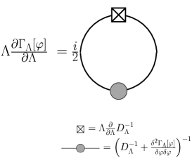
Figure 2: Graphical representation of the thermal renormalization group-equation (30).

Of course, in an interacting theory the full propagator is still a functional of the fields, making the equation impossible to solve exactly – nevertheless the existence of a pictorial description in terms of Feynman-like diagrams simplifies the discussion of the flow-equations and allows us to easily derive flow-equations for Green-functions etc.

One should note that in the context of thermal renormalization group-equations as in the usual real-time formalism one cannot generally dispose the thermal ghost fields ($\varphi_{2}$ in the above derivation). Even if one is only interested in Green-functions with physical ($\varphi_{1}$) external lines, the facts that equation (30) is formally of one-loop order and that the classical vertices do not mix the fields do not help since taking derivatives of (30) with respect to $\varphi_{1}$ introduces full vertices with external legs. These of course will in general mix physical and ghost-fields. Also note that $\Lambda\partial_{\Lambda}D_{\Lambda}^{-1}$ is a non-diagonal matrix. Since the insertion is basically treated like a vertex that mixes physical and ghost fields in (30) one gets contributions from all matrix-elements of the full propagator.

Finally, from the derivation given above it is immediately obvious that the general method of thermal renormalization group-equations is not restricted to thermal field theory in equilibrium. In principle one may use any form of density-matrices for the initial state. It is clear, however, that if the density-matrix is not bilinear in creation- and annihilation operators there will be $\Lambda$-dependent contributions also to the interaction terms in the path-integral (25) and the renormalization group-equation would not have a simple form. It is also straightforward to formulate thermal renormalization group-equations for gauge theories [13] or theories involving fermions.

Apart from the fact that the formulation of renormalization group-equations in the real-time approach to thermal field theories simplifies the calculation of real-time correlation functions since one avoids analytical continuation of quantities calculated at imaginary time arguments, the major difference between the thermal renormalization group formalism reviewed here and the Matsubara-approach by means of exact renormalization group-equations is the boundary condition for $\Lambda\rightarrow\infty$. As we have seen, the starting value for the effective action in the TRG-formulation is the full effective action at vanishing temperature. This should be contrasted to the imaginary-time approach where one treats quantum- and thermal fluctuations on equal footing. There the starting value for the effective action is the renormalized classical action. In practice this means that for a computation of finite-temperature quantities in terms of physical quantities at vanishing temperature a two-step procedure is necessary [25]. One first has to connect the parameters of the classical action to observables in a $T=0$-computation and only afterwards calculate quantities at finite temperature. To get control over the relation between e.g. perturbatively defined $\overline{\mbox{MS}}$-parameters and the corresponding couplings in the renormalization-scheme defined by the exact renormalization group approach one has to perform perturbative calculations also in the RG-approach [11]. In cases where one needs to go beyond one-loop order, this is an extremely cumbersome task [12]. In this respect the approach used in the present work is very convenient, since perturbative contributions at vanishing temperature may be taken into account by using perturbative starting conditions to any desired order. This feature implies of course an obvious limitation to the use of thermal renormalization group-equations in situations where already the theory at $T=0$ is strongly coupled. In such a situation one needs input from other nonperturbative methods such as lattice computations or exact renormalization group-equations at vanishing temperature. On the other hand this is a very welcome feature if one wants to study questions like the validity of perturbative dimensional reduction, a method that e.g. is at the heart of most of the present nonperturbative results on the electroweak phase-transition in the early universe [2] and is also studied in the context of QCD (for a review see e.g. [36]). In the case of the electroweak phase-transition there are a number of lattice studies that do not rely on perturbative dimensional reduction at least in the bosonic sector of the model (see for example [37] and references therein). A comparison of these results with studies assuming the validity of perturbative dimensional reduction indicates that method works fairly well in this sector [38]. However, to date there exist no nonperturbative checks of the method in the fermionic sector of the theory which is quantitatively important due to the large top-Yukawa coupling. TRG-equations should allow a test of this method also for models with chiral fermions.

2.2 Approximation schemes

Before presenting the results of our study of self-interacting scalar theories in the next section, we would finally like to briefly discuss some general strategies to approximately solve equations such as (30) [19]. The full effective action $\Gamma_{\Lambda}$ may be characterized by infinitely many couplings multiplying the invariants consistent with the symmetries of the theory under study. The functional differential equation (30) is thus equivalent to an infinite system of coupled nonlinear ordinary differential equations. Clearly one has to make some approximation to proceed. All approximations involve a truncation of the system of ordinary differential equations to another (possibly still infinite) system of equations by neglecting couplings.

The simplest approximations reduce the number of couplings considered to a finite set. A prominent example of such a truncation is the so-called ”local polynomial approximation” (LPA) to the effective potential, supplemented by a derivative expansion. This approximation is at the heart of most applications of Wilsonian RG-equations considered in the literature. It may be viewed as an expansion in the canonical dimension of the couplings (see [19]).

Alternatively one may consider truncations that keep an infinite set of couplings. This will result in (systems of) partial (integro-)differential equations. There are two more or less orthogonal ways to proceed:

1. One may perform a derivative expansion of the effective action. In this case one classifies the invariants by the number of derivatives appearing. The coefficients of these invariants are then functions of constant fields. Considering a scalar theory with one field $\varphi$ and $Z_{2}$-symmetry for simplicity, one expands the effective action as

   $$\Gamma_{\Lambda}=\int d^{d}x\left\{-V_{\Lambda}(\varphi^{2})+\frac{1}{2}Z_{\Lambda}(\varphi^{2})\left(\partial\varphi\right)^{2}+\frac{1}{2}Y_{\Lambda}(\varphi^{2})\left(u\cdot\partial\varphi\right)^{2}+...\right\}$$ (32)

   where we have taken into account the fact that at finite temperature Lorentz-invariance is broken by the rest-frame of the heat-bath and have introduced the corresponding four-vector $u_{\mu}$. Truncating the effective action at finite order in this expansion, one derives a set of coupled partial differential equations for the functions $V_{\Lambda}(\varphi^{2})$, $Z_{\Lambda}(\varphi^{2})$ etc.

   This is the approach that we will pursue below.

2. One may expand the effective action in powers of the fields,

   $$\Gamma_{\Lambda}=\left.\Gamma_{\Lambda}\right|_{\varphi=0}+\sum_{n=1}^{\infty}\frac{1}{n!}\int d^{d}x_{1}...d^{d}x_{n}\gamma_{\Lambda}^{(n)}(x_{1},...,x_{n})\varphi(x_{1})...\varphi(x_{n})$$ (33)

   The coefficients of this expansion are the 1PI Green-functions (the full propagators and vertices) of the theory. This is the strategy that is naturally followed in the study of Schwinger-Dyson equations [39].

The approach using the derivative expansion is technically relatively straightforward and has been used to study scalar theories in three dimensions [20, 21] and at finite temperature [31, 40], matrix-models [41], the abelian as well as an $SU(2)$-Higgs model in three dimensions [42], and an effective theory for low-energy QCD at finite temperature in the imaginary-time formalism [43]. It is generally appropriate in situations where the degrees of freedom considered correspond also to asymptotic states and the anomalous dimensions are small. As noted above one obtains a set of coupled partial differential equations for functions that depend on the invariants that one may construct from the fields considered (at vanishing momenta).

On the other hand, an expansion in the $n$-point functions rapidly becomes technically involved with growing $n$. Considering only the flow-equation for the two-point function of a scalar theory at $T=0$, one has to deal with a partial integro-differential equation of the structure

$$\Lambda\frac{\partial}{\partial\Lambda}\gamma_{\Lambda}^{(2)}(p^{2}) = \int\frac{d^{d}l}{(2\pi)^{d}}F_{4}\left[\gamma_{\Lambda}^{(2)}(l^{2}),\gamma_{\Lambda}^{(4)}(p^{2},l^{2},(lp))\right]+$$ (34)

$$+\int\frac{d^{d}l}{(2\pi)^{d}}F_{3}\left[\gamma_{\Lambda}^{(2)}((l+p)^{2}),\gamma_{\Lambda}^{(2)}(l^{2}),\gamma_{\Lambda}^{(3)}(p^{2},l^{2},(lp))\right]$$

corresponding to the diagrams depicted in figure 3. In a theory with vector-fields like QCD the number of invariants that make up a specific $n$-point function is rapidly growing with $n$. So far, this approach has been used to study the 2-point functions of pure Yang-Mills theory [44] and the four-point function of an effective model for QCD [45] (both at vanishing temperature).

Which of the above mentioned approaches should be considered depends on the physics of the theory under study. Generally, the derivative expansion will not be useful in situations where the momentum-dependence of the correlation functions is strongly modified by interactions.

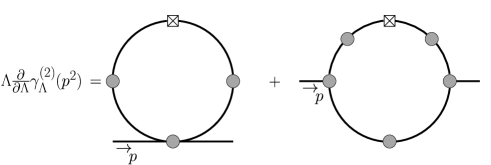
Figure 3: Exact flow-equation for the two-point function in a scalar theory.

After this more general review we will in the following section consider self-interacting scalar theories with an $O(N)$-symmetry at finite temperature.

3 Critical behavior of $O(N)$-symmetric scalar field theory

$O(N)$-symmetric scalar theories are well studied both in 4 dimensions at vanishing temperature as well as in statistical physics. The $O(N)$-symmetry of the action may be spontaneously broken at zero-temperature. In this case, one expects symmetry-restoration for large temperatures. The universal aspects of the corresponding phase-transition are very well known from considerations of the model in three Euclidean dimensions (for a review, see [18]). Quantities like the critical exponents are calculated to high orders in the $\epsilon$-expansion or in perturbation theory at fixed dimension $d=3$, where in both cases Borel-resummation has to be used to deal with the divergent series. There are also results from lattice studies available.

What is less well studied are the non-universal aspects like the critical temperature as a function of the zero-temperature ”physical” couplings. To study non-universal quantities one really has to consider the model at finite temperature. Perturbative studies of the theory at finite temperature are complicated by the bad infrared behavior near the phase-transition. Due to this behavior, for $N=1$ even super-daisy resummed perturbation theory falsely predicts a first-order phase-transition [4]. Alternatively, one may employ an expansion in $1/N$. In this case the resummation of daisy-diagrams yields exact results in leading order in $1/N$ [46] (see also [18]). One finds a second order phase-transition with mean-field values of the critical exponents $\beta$ and $\eta$, whereas $\nu=1+{\mathcal{O}}(1/N)$, $\delta=5+{\mathcal{O}}(1/N)$, $\alpha=-1+{\mathcal{O}}(1/N)$ and $\gamma=2+{\mathcal{O}}(1/N)$ (see below for definitions of the critical exponents).

As noted in the introduction, there are a number of methods that correctly predict a second-order phase-transition of the finite-temperature theory also for $N=1$. Results for the critical temperature have for example been given in [25, 29] and we will compare the corresponding values below.

3.1 Flow-equation for the effective potential

As stated in the last section, there is no way to solve the TRG-equation (30) exactly and we have to make simplifications. In the theory under consideration here, many studies have shown that a good truncation consists in performing a derivative expansion of the effective action and considering only the first few contributions. This fact is related to the smallness of the anomalous dimensions of the fields, which govern the scale-dependence of the wave-function renormalizations. In this spirit we will in the following approximate the effective action $\Gamma_{\Lambda}$ by its value for constant configurations, the effective potential $V_{\Lambda}$, and use a standard kinetic term. The effective potential is of course still a function of the fields. We may at this point use arguments given by [47] to simplify the task of calculating the effective potential considerably. The line of argument goes as follows: The free energy of the theory is given by the functional $\bar{\Gamma}_{\Lambda}[\varphi]$ which is defined as [47]

$$\frac{\delta\bar{\Gamma}_{\Lambda}[\varphi]}{\delta\varphi}=\left.\frac{\delta\Gamma_{\Lambda}[\varphi_{1},\varphi_{2}]}{\delta\varphi_{1}}\right|_{\varphi_{1}=\varphi_{2}=\varphi}$$ (35)

We are interested in the value of the effective action for constant field configurations and define the tadpole $\bar{\Gamma}_{\Lambda}^{(1)}(\varphi)$ through

$$\bar{\Gamma}_{\Lambda}^{(1)}(\varphi)=\left.\frac{\delta\Gamma_{\Lambda}[\varphi_{1},\varphi_{2}]}{\delta\varphi_{1}}\right|_{\varphi_{1}=\varphi_{2}=\varphi={\mathrm{const.}}}$$ (36)

By virtue of the symmetry

$$\Gamma_{\Lambda}[\varphi_{1},\varphi_{2}]=-\Gamma^{*}_{\Lambda}[\varphi_{2}^{*},\varphi_{1}^{*}]$$ (37)

one may derive relations between $n$-point functions with type-1 and type-2 external legs.

In the following we will discuss $O(N)$-symmetric scalar theories. We will label the physical- and thermal ghost-fields with subscripts as above, and use greek letters as superscripts to label the components of the $O(N)$-vectors ($\alpha,\beta,...=1...N$). We frequently use the $O(N)$-symmetry and write

$$\rho=\frac{1}{2}\varphi^{\alpha}\varphi^{\alpha}$$ (38)

Now consider the renormalization group-equation for the tadpole (36). Deriving equation (30) with respect to $\varphi_{1}^{\gamma}$ and setting the fields constant we obtain

$$\Lambda\frac{\partial}{\partial\Lambda}\frac{\delta\Gamma_{\Lambda}}{\delta\varphi_{1}^{\gamma}}(\rho) = \frac{i}{2}\int\frac{d^{4}k}{(2\pi)^{4}}{\mbox{tr}}\Biggl{\{}\left[-(\Delta_{0}-\Delta^{*}_{0})\frac{\Delta^{(\alpha)}_{\Lambda}\Delta^{(\alpha)*}_{\Lambda}}{\Delta_{0}\Delta^{*}_{0}}\Lambda\frac{\partial N_{f}(|\vec{k}|)}{\partial\Lambda}\left(\begin{array}[]{cc}1&1\\ 1&1\end{array}\right)\right]\delta^{\alpha\beta}\times$$ (44)

$$\qquad\quad\qquad\times\left(\begin{array}[]{cc}\frac{\delta^{3}\Gamma_{\Lambda}}{\delta\varphi_{1}^{\beta}\delta\varphi_{1}^{\alpha}\delta\varphi_{1}^{\gamma}}&\frac{\delta^{3}\Gamma_{\Lambda}}{\delta\varphi_{1}^{\beta}\delta\varphi_{2}^{\alpha}\delta\varphi_{1}^{\gamma}}\\ \frac{\delta^{3}\Gamma_{\Lambda}}{\delta\varphi_{2}^{\beta}\delta\varphi_{1}^{\alpha}\delta\varphi_{1}^{\gamma}}&\frac{\delta^{3}\Gamma_{\Lambda}}{\delta\varphi_{2}^{\beta}\delta\varphi_{2}^{\alpha}\delta\varphi_{1}^{\gamma}}\end{array}\right)\Biggr{\}}$$

where the trace is over the ”thermal” matrix-structure and we have used the fact that the two-point functions are diagonal with respect to the $O(N)$-indices. The term in square brackets constitutes the ”kernel” of the TRG-equation [9] and corresponds to the (modified) logarithmic derivative of the full (cutoff-)propagator with respect to $\Lambda$ (no sum over $\alpha$),

$$\left[-(\Delta_{0}-\Delta^{*}_{0})\frac{\Delta^{(\alpha)}_{\Lambda}\Delta^{(\alpha)*}_{\Lambda}}{\Delta_{0}\Delta^{*}_{0}}\Lambda\frac{\partial N_{f}(|\vec{k}|)}{\partial\Lambda}\left(\begin{array}[]{cc}1&1\\ 1&1\end{array}\right)\right] = \tilde{\partial}_{\ln\Lambda}\left(D_{\Lambda}^{-1}+\frac{\delta^{2}\Gamma_{\Lambda}}{\delta\varphi^{\alpha}\delta\varphi^{\alpha}}\right)^{-1}$$ (48)

$$=-\left(D_{\Lambda}^{-1}+\frac{\delta^{2}\Gamma_{\Lambda}}{\delta\varphi^{\alpha}\delta\varphi^{\alpha}}\right)^{-1}\left(\Lambda\frac{\partial}{\partial\Lambda}D_{\Lambda}^{-1}\right)\left(D_{\Lambda}^{-1}+\frac{\delta^{2}\Gamma_{\Lambda}}{\delta\varphi^{\alpha}\delta\varphi^{\alpha}}\right)^{-1}$$

where $\tilde{\partial}_{\ln\Lambda}$ denotes a derivative acting only on the explicit $\Lambda$-dependence of the free propagator $D_{\Lambda}^{-1}$.

Equation (44) is an obvious generalization of the case of one scalar field studied in [9, 31]. The trace yields

$${\mbox{tr}}\left(\begin{array}[]{cc}1&1\\ 1&1\end{array}\right)\left(\begin{array}[]{cc}\frac{\delta^{3}\Gamma_{\Lambda}}{\delta\varphi_{1}^{\beta}\delta\varphi_{1}^{\alpha}\delta\varphi_{1}^{\gamma}}&\frac{\delta^{3}\Gamma_{\Lambda}}{\delta\varphi_{1}^{\beta}\delta\varphi_{2}^{\alpha}\delta\varphi_{1}^{\gamma}}\\ \frac{\delta^{3}\Gamma_{\Lambda}}{\delta\varphi_{2}^{\beta}\delta\varphi_{1}^{\alpha}\delta\varphi_{1}^{\gamma}}&\frac{\delta^{3}\Gamma_{\Lambda}}{\delta\varphi_{2}^{\beta}\delta\varphi_{2}^{\alpha}\delta\varphi_{1}^{\gamma}}\end{array}\right) = \sum_{i,j=1}^{2}\frac{\delta^{3}\Gamma_{\Lambda}}{\delta\varphi_{i}^{\beta}\delta\varphi_{j}^{\alpha}\delta\varphi_{1}^{\gamma}}$$ (53)

$$= \frac{\delta^{2}}{\delta\varphi^{\beta}\delta\varphi^{\alpha}}\frac{\delta\bar{\Gamma}_{\Lambda}[\varphi]}{\delta\varphi^{\gamma}}$$ (54)

Now consider $i(\Delta_{0}-\Delta_{0}^{*})\frac{\Delta_{\Lambda}\Delta_{\Lambda}^{*}}{\Delta_{0}\Delta_{0}^{*}}$. The ”full” Feynman-propagator $\Delta_{\Lambda}$ reads

$$\Delta^{(\alpha)}_{\Lambda}=\frac{1}{k^{2}-m^{2}+\Pi^{(\alpha)}_{\Lambda}(k,\varphi)+i\epsilon}$$ (55)

where the self-energy is given by (no sum over $\alpha$)

$${\mathrm{Re}}\,\,\Pi_{\Lambda}^{(\alpha)}(k,\varphi) = {\mathrm{Re}}\left.\frac{\delta^{2}\Gamma_{\Lambda}}{\delta\varphi_{1}^{\alpha}(-k)\delta\varphi_{1}^{\alpha}(k)}\right|_{\varphi_{1}=\varphi_{2}=\varphi={\mathrm{const.}}}$$

$${\mathrm{Im}}\,\,\Pi_{\Lambda}^{(\alpha)}(k,\varphi) = \frac{1}{1+2N_{f}(|\vec{k}|)}{\mathrm{Im}}\left.\frac{\delta^{2}\Gamma_{\Lambda}}{\delta\varphi_{1}^{\alpha}(-k)\delta\varphi_{1}^{\alpha}(k)}\right|_{\varphi_{1}=\varphi_{2}=\varphi={\mathrm{const.}}}$$ (56)

To the considered order in the derivative expansion, the self-energies are momentum independent and real. Then in equation (44) we can replace [9]

$$i\left(\Delta_{0}-\Delta^{*}_{0}\right)\frac{\Delta^{(\alpha)}_{\Lambda}\Delta^{(\alpha)*}_{\Lambda}}{\Delta_{0}\Delta^{*}_{0}}\rightarrow 2\pi\delta\left(k^{2}-m^{2}+\Pi_{\Lambda}^{(\alpha)}(\varphi)\right)\Theta\left(|\vec{k}|^{2}+m^{2}-\Pi_{\Lambda}^{(\alpha)}(\varphi)\right)$$ (57)

and may use (37) to write (no sum over $\alpha$)

$$\Pi_{\Lambda}^{(\alpha)}(\varphi)=\frac{\delta^{2}\Gamma_{\Lambda}}{\delta\varphi_{1}^{\alpha}\delta\varphi_{1}^{\alpha}}=\frac{\delta^{2}\bar{\Gamma}_{\Lambda}}{\delta\varphi^{\alpha}\delta\varphi^{\alpha}}$$ (58)

We finally have to specify the form of the cut-off function $f_{\Lambda}$. In order to be able to do the loop-integral in (44) analytically, following [9, 31] we will choose this function such that

$$N_{f}(|\vec{k}|)=\frac{1}{e^{\beta\omega_{k}}-1}\Theta(|\vec{k}|-\Lambda)=N_{BE}(\omega_{k})\Theta(|\vec{k}|-\Lambda)$$ (59)

where $N_{BE}$ denotes the thermal distribution function for bosons. In this case we have $\partial_{\Lambda}N_{\Lambda}(|\vec{k}|)=N_{BE}(\omega_{k})\delta(|\vec{k}|-\Lambda)$ and the loop integrals are trivial.

We write for the functional $\bar{\Gamma}_{\Lambda}$

$$\bar{\Gamma}_{\Lambda}[\varphi]=\int d^{4}x\left\{\frac{1}{2}m^{2}\varphi^{2}-V_{\Lambda}(\varphi)+\frac{1}{2}Z_{\Lambda}(\varphi)\left(\partial\varphi\right)^{2}+\frac{1}{2}Y_{\Lambda}(\varphi)\left(u\cdot\partial\varphi\right)^{2}+...\right\}$$ (60)

and, working to lowest order in the derivative expansion, neglect $Z_{\Lambda}$ and $Y_{\Lambda}$. We will allow for spontaneous symmetry breaking along the ”1”-direction in the $O(N)$-group, giving rise to a radial (Higgs-) mode, the field $\varphi^{1}$, and $N-1$ Goldstone-modes $\varphi^{\alpha\neq 1}$. This amounts to evaluating the effective action on a background field configuration $\varphi^{\alpha}=\sqrt{2\rho}\delta^{\alpha 1}+\chi^{\alpha}(q)$ and putting $\chi^{\alpha}=0$ at the end. We then have (no sum over $\alpha$)

$$\Pi_{\Lambda}^{(\alpha)}(\rho)=m^{2}+\frac{\partial^{2}V_{\Lambda}(\rho)}{\partial\varphi^{\alpha}\partial\varphi^{\alpha}}$$ (61)

Dropping the subscript $\Lambda$ we find from (44)

$$\Lambda\frac{\partial}{\partial\Lambda}\frac{\partial V(\rho)}{\partial\varphi^{\gamma}} = -\frac{\Lambda^{3}}{4\pi^{2}}\frac{N_{BE}(\omega_{1})}{\omega_{1}}\frac{\partial^{3}V(\rho)}{\partial\varphi^{\gamma}\partial\varphi^{1}\partial\varphi^{1}}\Theta(\omega_{1}^{2})-$$ (62)

$$-(N-1)\frac{\Lambda^{3}}{4\pi^{2}}\frac{N_{BE}(\omega_{2})}{\omega_{2}}\frac{\partial^{3}V(\rho)}{\partial\varphi^{\gamma}\partial\varphi^{2}\partial\varphi^{2}}\Theta(\omega_{2}^{2})$$

$\omega_{1}$ and $\omega_{2}$ denote the frequencies of the radial and the Goldstone-modes respectively, i.e.

$$\omega_{1}=\sqrt{\Lambda^{2}+\frac{\partial^{2}V}{\partial\varphi^{1}\partial\varphi^{1}}}=\sqrt{\Lambda^{2}+V^{\prime}(\rho)+2\rho V^{\prime\prime}(\rho)}\quad;\quad\omega_{2}=\sqrt{\Lambda^{2}+\frac{\partial^{2}V}{\partial\varphi^{2}\partial\varphi^{2}}}=\sqrt{\Lambda^{2}+V^{\prime}(\rho)}$$ (63)

where primes denote derivatives with respect to $\rho$. We may finally integrate eq. (62) with respect to $\varphi^{\gamma}$ to obtain the flow-equation for the effective potential as

$$\Lambda\frac{\partial}{\partial\Lambda}V(\rho) = -T\frac{\Lambda^{3}}{2\pi^{2}}\ln\left[1-\exp\left(-\beta\sqrt{\Lambda^{2}+V^{\prime}(\rho)+2\rho V^{\prime\prime}(\rho)}\right)\right]\Theta(\Lambda^{2}+V^{\prime}(\rho)+2\rho V^{\prime\prime}(\rho))-$$ (64)

$$-(N-1)T\frac{\Lambda^{3}}{2\pi^{2}}\ln\left[1-\exp\left(-\beta\sqrt{\Lambda^{2}+V^{\prime}(\rho)}\right)\right]\Theta(\Lambda^{2}+V^{\prime}(\rho))$$

We will in the numerical evaluation also use the flow-equation for the minimum of the potential in the spontaneously broken phase, $\rho_{0}$. This is obtained from the condition $\left.V^{\prime}(\rho)\right|_{\rho_{0}}=0$ and reads

$$\Lambda\frac{\partial\rho_{0}}{\partial\Lambda} = \frac{\Lambda^{3}}{4\pi^{2}}\left(3+2\frac{\rho_{0}V_{0}^{(3)}}{V_{0}^{\prime\prime}}\right)\frac{1}{\sqrt{\Lambda^{2}+2\rho_{0}V_{0}^{\prime\prime}}}\frac{1}{\exp\sqrt{\frac{\Lambda^{2}}{T^{2}}+\frac{2\rho_{0}V_{0}^{\prime\prime}}{T^{2}}}-1}\Theta(\Lambda^{2}+2\rho_{0}V_{0}^{\prime\prime})+$$ (65)

$$+(N-1)\frac{\Lambda^{3}}{4\pi^{2}}\frac{1}{\Lambda}\frac{1}{\exp\sqrt{\frac{\Lambda^{2}}{T^{2}}}-1}$$

As we will see shortly, it is also convenient to define dimensionless quantities in the following way:

$$\lambda=\frac{\Lambda}{T}\quad;\quad\kappa=\frac{\rho}{\Lambda T}\quad;\quad u=\frac{V}{\Lambda^{3}T}\quad;\quad\frac{d^{i}V}{d\rho^{i}}=\Lambda^{3-i}T^{1-i}\frac{d^{i}u}{d\kappa^{i}}$$ (66)

The corresponding flow-equations read

$$\lambda\frac{\partial u}{\partial\lambda} = -3u+u^{\prime}\kappa-\frac{1}{2\pi^{2}}\ln\left[1-\exp\left(-\lambda\sqrt{1+u^{\prime}+2\kappa u^{\prime\prime}}\right)\right]\Theta(1+u^{\prime}+2\kappa u^{\prime\prime})-$$ (67)

$$\qquad\quad-\frac{N-1}{2\pi^{2}}\ln\left[1-\exp\left(-\lambda\sqrt{1+u^{\prime}}\right)\right]\Theta(1+u^{\prime})$$

and

$$\lambda\frac{\partial\kappa_{0}}{\partial\lambda} = -\kappa_{0}+\frac{\lambda}{4\pi^{2}}\left(3+2\frac{\kappa_{0}u_{0}^{(3)}}{u_{0}^{\prime\prime}}\right)\frac{1}{\sqrt{1+2\kappa_{0}u_{0}^{\prime\prime}}}\frac{1}{e^{\lambda\sqrt{1+2\kappa_{0}u_{0}^{\prime\prime}}}-1}\Theta(1+2\kappa_{0}u_{0}^{\prime\prime})+$$ (68)

$$\qquad+(N-1)\frac{\lambda}{4\pi^{2}}\frac{1}{e^{\lambda}-1}$$

As was already pointed out in [9, 31], if one considers the limit where $\Lambda^{2}+V^{\prime}+2\rho V^{\prime\prime}$ and $\Lambda^{2}+V^{\prime}$ are both $\ll T^{2}$ one recovers the flow-equations of the purely three-dimensional theory with a sharp cutoff up to a field independent contribution. This is the relevant limit in the scaling-regime close to the phase-transition and motivates the use of the rescaled variables defined in (66). The powers of the temperature appearing in eq.s (66) are identical to those obtained by naive dimensional reduction, whereas the powers of $\Lambda$ are the ones one would use in the purely three-dimensional theory to make the couplings dimensionless.

We finally have to give the starting value for the effective potential in the limit $\Lambda\rightarrow\infty$. As discussed in section 2, the effective action in this limit becomes the effective action of the zero-temperature theory. Correspondingly the starting value for the effective potential should be the full effective potential of the theory at vanishing temperature. At this point we face an obvious problem if we are to use perturbative results on this quantity. Consider the effective potential of an $O(N)$-symmetric scalar theory in the broken phase at $T=0$ as computed e.g. in the $\overline{MS}$-scheme. Taking the scale to be set by the zero-temperature tree-level Higgs-mass $m_{0}^{2}=2g\rho_{0}$ to one loop we have

$$V_{T=0}(\rho) = -g\rho_{0}\rho+\frac{g}{2}\rho^{2}+\frac{g^{2}}{64\pi^{2}}\left(3\rho-\rho_{0}\right)^{2}\left[\ln\frac{3\rho-\rho_{0}}{2\rho_{0}}-\frac{3}{2}\right]+$$ (69)

$$\qquad+(N-1)\frac{g^{2}}{64\pi^{2}}\left(\rho-\rho_{0}\right)^{2}\left[\ln\frac{\rho-\rho_{0}}{2\rho_{0}}-\frac{3}{2}\right]$$

On the right hand side of the flow-equation (64) we need the first two derivatives of the potential with respect to $\rho$ at arbitrary values of the field. Now from equation (69) it is obvious that the second derivative of the potential has logarithmic singularities at $\rho=\frac{\rho_{0}}{3}$ and, for $N>1$, at $\rho=\rho_{0}$. This is of course a well known fact which for example forces us to define the renormalized quartic coupling in the massless theory with $N=1$ away from the point $\rho=0$ [48]. As long as we work with a polynomial expansion, i.e. as long as we choose to write the potential as

$$V(\rho)=V(\tilde{\rho})+\sum\frac{V^{(n)}}{n!}(\rho-\tilde{\rho})^{n}$$ (70)

and derive flow-equations for the couplings $V^{(n)}$, this is no problem. For $N=1$ we may use $\tilde{\rho}=\rho_{0}$, for $N>1$ one may still proceed as long as one does not expand the potential about its minimum. Even in that case, we could in principle avoid any infrared problems by using the perturbative effective potential evaluated with an infrared cut-off in the loop integration. This would compare closely to the approach followed in [25], where a local polynomial approximation was used for the potential and the zero-temperature renormalized couplings were defined at some non-vanishing scale. In this work we will restrict ourselves to small values of the zero-temperature couplings and neglect the quantum-corrections to the effective potential, that is we use as a starting value for the integration of the flow-equation (64) the tree-level potential

$$V_{\Lambda_{0}}(\rho)=-g\rho_{0}\rho+\frac{g}{2}\rho^{2}$$ (71)

This simplification has of course no effect on the universal aspects of the critical behavior such as the critical exponents, certain ratios of critical amplitudes or the scaling equation of state. For non-universal quantities such as the critical temperature we will have corrections from the (logarithmic) four-dimensional running of the couplings. These corrections should however be small for the values of the couplings considered in the present work. We now discuss the results of a solution of the flow-equations given in (64), (65), (67) and (68) with the starting value given by (71) (or the corresponding scaled potential according to (66)) for different values of $N$. For the numerical work, the methods proposed in [49] are used.

3.2 Numerical results

We start by discussing the results for the case of one scalar field, corresponding to the Ising model of statistical mechanics. The first question concerns the order of the phase-transition. As was already pointed out above, daisy-resummed perturbation theory fails in predicting the correct critical behavior of the theory in this case. In the framework of thermal renormalization group-equations, the case $N=1$ has already been addressed in [9, 31], where the transition was found to be second order and critical exponents have been given.

We display the dependence of the minimum of the potential on the external scale $\Lambda$ at different temperatures in figure 4.

Figure 4: Upper panel: The dimensionless minimum as a function of $\ln{\Lambda/T}$ for various values of the temperature around $T_{c}$. For temperatures above $T_{c}$ the minimum vanishes at some finite scale $\Lambda_{\mathrm{symm}}$, for $T<T_{c}$ the dimensionless minimum diverges as $\Lambda\rightarrow 0$. Lower panel: The dimensionful minimum $\rho_{0}$ (in units of $\rho_{0}(T=0)$) as a function of $\Lambda/T$. For temperatures below the critical temperature the dimensionful minimum approaches a constant value that is a decreasing function of the temperature until it vanishes at $T_{c}$ as $\Lambda\rightarrow 0$. For low temperatures thermal fluctuations play effectively no rôle and $\rho_{0}$ almost remains at the starting value.

In the upper panel, the dimensionless minimum $\kappa_{0}$ is displayed as a function of $\ln\frac{\Lambda}{T}$ for several temperatures around the critical one (we have chosen $g=0.1$ here). We start the evolution of the potential at some large value of $\Lambda/T$ in the broken phase, where $\rho_{0}(T=0)$ is used to set the scale and all dimensionful quantities are given in units of $\rho_{0}(T=0)$. For temperatures larger than the critical one (solid lines), the minimum vanishes at some nonzero scale $\Lambda_{\mathrm{symm}}$ and the theory is in the symmetric phase. On the other hand, for temperatures below $T_{c}$ the dimensionful minimum $\rho_{0}$ approaches some constant as $\Lambda\rightarrow 0$ (this is seen in the lower panel of fig. 4, where we display the dimensionful minimum as a function of $\Lambda/T$). According to (66) $\kappa_{0}$ then diverges. We see from figure 4 that at the critical temperature, the dimensionless minimum asymptotically reaches a finite nonvanishing value, $\kappa^{*}_{0}$. As is expected from dimensional reduction and was explicitly demonstrated in [31], this value is the fixed-point value of the corresponding three-dimensional theory. The phase-transition is of second order and the theory is in the universality class of the three-dimensional Ising model. Before turning to the universal behavior of the theory, let us briefly discuss the critical temperature as a function of the zero-temperature coupling. Our results on this quantity are displayed in figure 5, where we plot the ratio of $T_{c}$ and the naive perturbative result, given by

$$T_{c,1-{\mathrm{loop}}}=\sqrt{\frac{24}{N+2}}\sqrt{\rho_{0}}$$ (72)

as solid line and compare to the values found in the ERG-approach in the Matsubara-formalism in [25] as squares. We find good agreement as expected.

Figure 5: The ratio $T_{c}/T_{c,1-{\mathrm{loop}}}$ as a function of the zero-temperature coupling $g$ for $N=1$. For comparison results from [25] are also given (squares).

We finally discuss the results on the universal behavior as obtained from the TRG. The universal critical behavior of a given field theory is summarized in a number of critical exponents, certain ratios of critical amplitudes, and the scaling equation of state (see e.g. [18]). We will start by discussing critical exponents and amplitudes. These quantities encode the behavior of different observables as the temperature approaches its critical value. Specifically, we will consider the following quantities:

1. The (unrenormalized) mass of the order-parameter field (in the language of statistical mechanics the inverse magnetic susceptibility in zero field). The susceptibility diverges at the phase-transition, corresponding to a behavior of the mass according to

   $$M_{\pm}^{2}=\left(C_{\pm}\right)^{-1}\left|\frac{T_{c}-T}{T_{c}}\right|^{\gamma}$$ (73)

   This defines the critical exponent $\gamma$ and the amplitudes $C_{\pm}$. The ratio $C_{+}/C_{-}$ is a universal quantity.

2. The quartic coupling $g(\Lambda\rightarrow 0)$ goes to zero at the critical temperature according to

   $$g_{\pm}=\ell_{\pm}\left|\frac{T_{c}-T}{T_{c}}\right|^{\nu}$$ (74)

   The exponent $\nu$ also governs the behavior of the renormalized mass at the critical temperature. Since we have approximated the wave-function renormalizations to be constant, $\nu$ should be equal to $\gamma/2$.

3. The dimensionful minimum of the effective potential (corresponding to the spontaneous magnetization) approaches 0 as the temperature approaches $T_{c}$ from below, where

   $$\varphi_{0}=B\left(\frac{T_{c}-T}{T_{c}}\right)^{\beta}$$ (75)

4. Finally, the behavior of the effective potential at the critical temperature is described for small values of $\rho$ by (remember $\varphi=\sqrt{2\rho}$)

   $$\frac{\partial V}{\partial\varphi}=D\varphi^{\delta}$$ (76)

We stress that we are considering the theory explicitly at finite temperature. Thus one may expect the scaling behavior encoded in the critical exponents only in the region where dimensional reduction is effective. The relation (76) will for example not hold for large $\varphi\>\hbox to-0.2pt{\lower 2.5pt\hbox{$\sim$}\hss}{\raise 3.0pt\hbox{$>$}}\>T$ where the three-dimensional limit is not reached. Effective exponents taking into account this ”dimensional crossover” are discussed for example in [6] and the second reference of [27]. Our results for the critical exponents defined above are given in table 1, the results for some critical amplitude-ratios and critical couplings are displayed in table 2. In both tables, we give results obtained by other approaches for comparison. Let us make some comments regarding the results presented in the tables. We should first note that the exponents may, apart from the possibility discussed above, also be determined from the scaling equation of state to be discussed below. We have in particular obtained the value of $\delta$ in this way. The value is completely consistent with $\delta=5$ which was found using the thermal renormalization group, but extracting $\delta$ according to the above definition, eq. (76) in [31]. In fact, one can show that $\delta=5$ is the exact solution to the fixed-point equations in the three-dimensional theory in lowest order in the derivative expansion [50].

	$\beta$	$\gamma$	$\delta$	$\eta$	$\nu$
This work	0.345	1.37	4.97	–	0.67
TRG+LPA [9]			3.57	0.015	0.58
3d ERG + LPA [19]	0.333	1.247		0.045	0.638
3d ERG [20]	0.336	1.258	4.75	0.044	0.643
3d ERG + WFR [21]	0.330	1.232		0.047	0.631
Best values [18]	0.325	1.240	4.81	0.032	0.630

Table 1: Critical exponents from different approaches ($N=1$)

The other exponents given in the table have been determined in a number of ways: We have determined $\beta$ from (75) above and from the scaling equation of state and find values of $0.3458$ and $0.3451$, identical within the numerical accuracy. $\gamma$ was obtained from the definition given in (73) and from the asymptotic behavior of the Widom scaling function parametrizing the equation of state and we find $1.369$ from the EOS, $1.368$ from (73) if $T_{c}$ is approached from above and $1.369$ if we approach the critical temperature from below. Finally $\nu$ is obtained from (74) to be $0.679$ coming from $T>T_{c}$ and $0.663$ for $T\rightarrow T_{c}$ from below. All in all the critical exponents are rather robust with respect to details of the numerical procedure. The deviation from the best values given also in table 1 is due to the approximations made in reducing the exact renormalization group-equation to the flow-equation for the effective potential, eq. (64), namely the neglect of higher orders in the derivative expansion. This also prevents us from studying the critical exponent $\eta$ which is defined as the anomalous dimension at the critical temperature as $\Lambda\rightarrow 0$. From the table it is also clear that we could improve on the results for the exponents and amplitudes by taking into account the wave-function renormalizations, as has been done in the work listed as ERG in table 1. In [19] the potential was expanded around the minimum and only a finite number of couplings was kept (LPA). On the other hand, the authors went beyond leading order in the derivative expansion. The LPA was dropped in [20], where however the wave-function renormalization was still assumed to be field independent. This approximation is finally also given up in [21]. We should keep in mind that all these results were obtained in the framework of a three-dimensional effective theory rather than in the full temperature-dependent problem.

	$C_{+}/C_{-}$	$R_{\chi}$	$\lambda_{4*}$	$\lambda_{6*}$	$B$	$C_{+}$	$D$
					$(g_{T=0}=0.1)$
This work	4.50	1.76	19.6	1725	1.05	0.54	2.73
3d ERG + LPA [19]			27.8	1311
3d ERG [20]	4.29	1.61
3d ERG + WFR [21]	4.966	1.647
Monte-Carlo [23]			23.3	1476
Best values [18]	4.95	1.65

Table 2: Critical amplitude ratios and couplings from different approaches ($N=1$). The last three entries are non-universal.

Let us now discuss the results presented in table 2. Here we give the universal ratios of critical amplitudes $C_{+}/C_{-}$ and $R_{\chi}$ as well as the universal critical couplings $\lambda_{4*}$ and $\lambda_{6*}$ and the non-universal amplitudes $B$, $C_{+}$ and $D$ for $g_{T=0}=0.1$. The definition of $C_{\pm}$ has been given in (73). $R_{\chi}$ is a universal combination of several non-universal quantities and reads

$$R_{\chi}=C_{+}DB^{\delta-1}$$ (77)

We have extracted the numbers for the amplitudes used here from the equation of state to be discussed below. We have also extracted the ratio $C_{+}/C_{-}$ from the behavior of the unrenormalized mass as given in (73). In this case we find $C_{+}/C_{-}=4.58$, consistent with the value quoted in the table. As noted in the discussion of the critical exponents, also in the case of the amplitudes the major source of error is the derivative expansion used here, as may be seen by again comparing with the results given in [21].

The universal critical couplings given in the table are defined by

$$V(\varphi)=\sum_{n=2}^{\infty}\frac{\lambda_{n}}{n!}\varphi^{n}$$ (78)

and are taken at the critical temperature, i.e. in the scaling limit. $\lambda_{4*}$ and $\lambda_{6*}$ are thus simply related to the second and third derivative of the potential at the critical temperature with respect to $\rho$. The values given for comparison have been found through the ERG, using a local polynomial expansion and on the lattice, in both cases working in three dimensions.

Let us then turn to the scaling equation of state. In the language of statistical mechanics the equation of state relates the temperature, the order parameter and the external field. In the present setting, the external field $H$ is given by $H=V^{\prime}(\rho)\varphi$ and the equation of state has the following scaling form:

$$\frac{\partial V}{\partial\rho}=\left(\sqrt{2\rho}\right)^{\delta-1}f(x)\qquad;\qquad x=\frac{T-T_{c}}{T_{c}}\left(\sqrt{2\rho}\right)^{-1/\beta}$$ (79)

The function $f(x)$ is known as the Widom scaling function and is universal up to normalization and a rescaling of $x$. It encodes information about the universal critical behavior and several amplitudes and critical exponents may be obtained from $f$ in different limits. For the amplitudes and exponents treated above we have the following relations involving the equation of state: The value of $f$ at $x=0$ gives the amplitude $D$,

$$\lim_{x\rightarrow 0}f(x)=D$$ (80)

The asymptotic behavior of $f$ in the symmetric phase is

$$\lim_{x\rightarrow+\infty}f(x)=\left(C_{+}\right)^{-1}x^{\gamma}$$ (81)

The amplitude $B$ and the critical exponent $\beta$ are related to the zero of $f$ in the broken phase through

$$f\left(-B^{-1/\beta}\right)=0$$ (82)

and the amplitude $C_{-}$ is obtained from the zero of $f$ and the value of the derivative at the zero through

$$\left(C_{-}\right)^{-1}=\frac{1}{\beta}f^{\prime}\left(-B^{-1/\beta}\right)B^{\delta-1-\frac{1}{\beta}}$$ (83)

We have pointed out that the normalization of $f$ and of $x$ are non-universal. We will in the following figures compare our results with results from exact renormalization group-equations in three dimensions [20] and with results from Monte-Carlo simulations in the broken [24] and in the symmetric phase [23] (figure 6).

Figure 6: The logarithm of the Widom scaling function $f(x)$ for $N=1$ (solid lines). The left panel shows $f(x)$ in the broken phase, corresponding to $x<0$ whereas the right panel gives $f$ in the symmetric phase. The short dashed lines are from the ERG in three dimensions [20], the long dashed lines give results from lattice simulations (broken phase: [24], symmetric phase: [23]).

In order to do so, we fix the normalization by demanding equality of the results given in form of a numerical fit in [20] and approximate polynomial expressions in [24, 23] with our results for 2 values of $x$. Since the lattice simulations used for the comparison were obtained on different lattices we have used different rescalings for the Monte-Carlo results in the left and right panels in figure 6, corresponding to the broken and symmetric phase respectively. In order to have a fair comparison also of the results from [20] with the lattice results in both phases, we have also rescaled these results differently in both panels.

In principle, for a comparison of our results with the ones of [20] we only have two free parameters corresponding to two values of $x$ where equality may be imposed. Thus we also present in figure 7 a comparison of our curve with the curve given by [20] for different normalizations: The solid line in figure 7 corresponds to our result in the symmetric phase, the short dashed line is the same as in the right panel of figure 6, obtained by equating the results at two values of $x$ in the symmetric phase, whereas the dashed-dotted line is the result from [20] if we use the two values of $x$ from the broken phase (left panel of fig. 6) for normalization for the whole range of $x$.

Figure 7: $f(x)$ for $N=1$ in the symmetric phase compared to the three-dimensional ERG results from [20] for different normalizations (see text for details).

The curves obtained in this work and the results given in [20] are almost identical in the broken phase (left panel of fig. 6) and show only a slight deviation in the symmetric phase for large $x$, connected to the different results for the critical exponent $\gamma$ (see table 1). The agreement with the results from lattice simulations is rather satisfactory, as was already noted in [31] for the broken phase. In view of the sizable deviations of results obtained in the framework of the $\epsilon$-expansion or other perturbative approaches from the lattice results, this is a nontrivial achievement. The deviation in the asymptotic behavior for large positive $x$ in figure 6 is of no concern. In this region the approximate polynomial expression given in [23] is incompatible with the known behavior corresponding to (81) – it would give an exponent $\gamma=2$ in contrast to the known results (table 1).

After presenting detailed results for $N=1$, we now proceed to a study of the case $N=4$. This case is interesting, since the is expected to govern the universal behavior of the two-flavor chiral phase-transition in the chiral limit. The arguments in favor of this conjecture rely on dimensional reduction and the fact that in the imaginary-time formulation the fermionic degrees of freedom obey anti-periodic boundary conditions and thus have no static modes. The infrared behavior should then be dictated by the bosonic excitations alone, which in this case are the pions and the ”sigma” (for a more complete discussion of the chiral phase-transition in the two-flavor case also away from the chiral limit in the imaginary-time formalism see e.g. [43]). We should also mention that due to the existence of massless degrees of freedom also in the broken phase away from the critical temperature perturbative calculations for $N>1$ are even more infrared problematic then for the case discussed above.

We start our discussion by plotting the critical temperature as a function of the zero-temperature coupling $g(T=0)$ in figure 8 (solid line). We again display for comparison the values obtained by Tetradis and Wetterich [25]. As for the case $N=1$ we find excellent agreement of the results.

Figure 8: The ratio $T_{c}/T_{c,1-{\mathrm{loop}}}$ as a function of the zero-temperature coupling $g$ for $N=4$. For comparison results from [25] are also given.

Next we turn to the critical equation of state. This is displayed in figure 9, where as for $N=1$ we display $\ln(f)$ as a function of $\ln(x)$ in the symmetric phase ($x>0$) in the right panel and as a function of $\ln(-x)$ in the broken phase ($x<0$) in the left panel. As discussed above one obtains critical exponents and amplitudes from the scaling function, and we collect the values together with some results from other approaches in tables 3 and 4.

Figure 9: The Widom scaling function for $N=4$ (solid line) in the broken (left panel) and the symmetric (right panel) phase. For comparison we give the suitably normalized results from [51] (dashed line).

Considering the Widom scaling function, we again observe from figure 9 almost perfect agreement of our result (the solid curve) with results from the ERG given in [51] (dashed curve) in the broken phase. In the symmetric phase, there is a slight deviation for large $x$, which again is due to the different values found for the exponent $\gamma$ (table 3). In figure 9, we have normalized the results from [51] to our results for two positive values of $x$ close to $x=0$. A comparison of the results from the ERG and results from other approaches including lattice and $\epsilon$-expansion may be found in [51] and again shows that the lattice results on the equation of state compare well with results from the Wilson renormalization group, whereas the $\epsilon$-expansion differs from the Monte-Carlo results.

	$\beta$	$\gamma$	$\delta$	$\eta$	$\nu$
This work	0.433	1.73	5.0	–	0.86
3d ERG + LPA [19]	0.409	1.556		0.034	0.791
ITF ERG [51]	0.407	1.548	4.80	0.0344	0.787
3d PT [52]	0.38	1.44	4.82	0.03	0.73
3d MC [53]	0.384	1.48	4.85	0.025	0.748

Table 3: Critical exponents from different approaches ($N=4$)

	$C_{+}/C_{-}$	$R_{\chi}$	$\lambda_{4*}$	$\lambda_{6*}$	$B$	$C_{+}$	$D$
					$(g_{T=0}=0.1)$
This work	–	1.38	9.4	475	1.81	0.0797	1.62
ITF ERG [51]	–	1.02

Table 4: Critical amplitude ratios and couplings from different approaches ($N=4$). The last three entries are non-universal.

For the critical exponents given in table 3 we note a slightly larger deviation of our values from those obtained from the lattice [53] or from higher order perturbation theory [52]. Although the values obtained from the ERG in different approximations also show a larger deviation than was obtained for $N=1$, in the case $N=4$ our results differ also from the ERG-results by up to $10\%$. There are a number of reasons for this deviation. First, as in the case of $N=1$ the derivative expansion induces an error in the critical exponents. We expect the error from the neglect of the wave-function renormalization $Z_{\Lambda}$ to be responsible for most of the difference between the values found in the present work and the ones given in [19] and [51]. We have also checked in the three-dimensional effective theory and using the local polynomial expansion for the effective action how much the choice of a $\Theta$-function cutoff in (59) affects the result (in lowest order in the derivative expansion). In principle, the choice of the cutoff-function has no effect on the results if one solves the full RG-equation. Since we have to make approximations, a slight cutoff-dependence is expected. In the case we have checked, the results for the critical exponents using a sharp cutoff and using an exponential cutoff as usually used in the framework of the ERG differ by about $3\%$.

There is however an additional contribution in first order in the derivative expansion for $N>1$, being of the structure $\tilde{Z}_{\Lambda}(\rho)\varphi^{\alpha}\varphi^{\alpha}\partial^{2}\varphi^{\beta}\varphi^{\beta}$. This term should account for much of the remaining difference to the exact exponents.

The same remarks apply to the universal amplitude-ratio $R_{\chi}$ which is compared to the value found in [51] in table 4. In view of these uncertainties the values for the exponents and amplitudes found in the present work are consistent with the expectations, although they certainly leave room for improvement along the lines discussed above.

Finally, we consider the $N$-dependence of the critical temperature to compare with the leading order result of the large-$N$ expansion. In figure 10 we have plotted our values for $g(T=0)=0.1$ as a function of $N$, where again the critical temperatures are given in units of $\sqrt{\rho_{0}}$ (solid line).

Figure 10: $T_{c}$ in units of $\sqrt{\rho_{0}}$ as a function of $N$ for $g(T=0)=0.1$ (solid line). For comparison results from [25] (squares), and the result of an expansion in $1/N$ are also given. Our results are very well reproduced by the naive perturbative result (72) for all $N$.

For comparison, the dashed line shows the result that is obtained in leading order in $1/N$ [46]

$$T_{c}=\sqrt{\frac{24}{N}}\sqrt{\rho_{0}}+{\mathcal{O}}\left(\frac{1}{N^{2}}\right)$$ (84)

Naive perturbation theory yields (72) which is consistent with our results on the level of $1-2\%$ for the small value of $g_{T=0}=0.1$ choosen here (see figures 5 and 8 for a comparison of $T_{c}$ with (72) as a function of the coupling). Also given are the results from the ERG in the imaginary-time formulation [25] as squares. Again we observe good agreement as was already seen in figures 5 and 8. It is interesting that we can also study the limit $N\rightarrow 0$ straightforwardly.

4 Conclusions and outlook

In the present paper we have discussed the finite-temperature phase-transitions of self-interacting scalar theories with at vanishing temperature spontaneously broken $O(N)$-symmetry. We have used an implementation of the Wilsonian renormalization group-approach for field theory in thermal equilibrium in the Schwinger-Keldysh (CTP)-formulation [9].

We have reviewed and discussed this “thermal renormalization group” (TRG)-approach in section 2. The approach has a number of advantages as compared to the more common RG-approach in the framework of imaginary-time thermal field theory: It allows for the direct computation of real-time observables in field theory at finite temperature, avoiding the need for analytical continuation. Thus quantities like thermal damping rates and the like are easily accessible and first results may be found in the literature [10]. As the imaginary-time RG approach, the method is non-perturbative and allows for the treatment of situations in which perturbation theory fails, which is typically the case near second order phase-transitions or in strongly coupled theories.

Since the real-time formulation of thermal field theory clearly distinguishes thermal and quantum-fluctuations and the TRG treats only the thermal fluctuations, one obtains a direct connection between the physical couplings of the theory at vanishing and at non-vanishing temperature and there is no need to take into account zero-temperature renormalization scheme dependencies. Furthermore the TRG manifestly respects gauge-invariance.

Finally, after a straightforward generalization of the formalism given in section 2, the TRG may easily be applied to field theory at finite density (chemical potential) or to theories with a non-thermal density matrix. The method thus offers a nonperturbative approach for the study of a number of interesting questions in field theory in a hot and possibly dense environment.

The main part of the present work is concerned with the application of this formalism to $O(N)$-symmetric scalar theories in $3+1$ dimensions at temperatures near to the critical one. We have given extensive discussions of the cases $N=1$ and $N=4$, being especially interesting for a number of reasons. The case $N=1$ in three dimensions corresponds to the well known Ising-model. The electroweak sector of the standard model is in the universality-class of the Ising model if the zero-temperature Higgs mass is at its critical value $\sim 70$ GeV [17].

We have given the critical temperature in terms of the scalar self-coupling at $T=0$ and found good agreement with results found from the exact renormalization group in the imaginary-time formulation [25] (figure 5). The results disagree with the values found in the environmentally friendly RG [29] but are consistent with results from the auxiliary mass method [30], where the latter yields results that are basically identical to the perturbative values for couplings up to $g=1/3$ (figure 3 of the last reference of [30]). Although the approach of [29] differs from the one used in the present work, the discrepancies of the results on the critical temperature are somewhat surprising and should be further understood.

We have then at length discussed the critical behavior of the theory, focusing on the universal aspects encoded in critical exponents, amplitude ratios and the scaling equation of state (tables 1 and 2, figures 6 and 7). Whereas the exponents found in the present work are not as accurate as the results found from Borel-resummed $\epsilon$-expansion and other methods working directly in the three-dimensional effective model, the scaling equation of state compares very favorably with results from Monte-Carlo simulations in three dimensions. This demonstrates the power of the TRG and also demonstrates explicitly in a nonperturbative context how the critical behavior of the finite temperature theory is governed by the three-dimensional Euclidean model.

After the discussion of $N=1$ we have turned to the case $N=4$, which is presumably in the same universality-class as the chiral phase-transition in the case of 2 massless flavors. We find a similar situation as in the case of $N=1$: The critical temperatures are compatible with the results from the ERG in imaginary-time [25] (figure 8). For this case, results from the environmentally friendly RG or the auxiliary mass method are not available.

Concerning the critical behavior, we again find a scaling form of the equation of state in very good agreement with the results from the exact renormalization group as given in [51] (figure 9) but a somewhat larger difference in the critical exponents and amplitude-ratios (tables 3 and 4). We have argued that this situation should improve going to higher order in the derivative-expansion.

Finally we have given the critical temperature as a function of $N$ for a large range of $N$, using a small value of the zero-temperature coupling $g_{T=0}=0.1$ (figure 10). We are able to study the limit $N\rightarrow 0$, which is of interest for statistical physics and find results consistent with the values obtained from the exact renormalization group in the imaginary-time formulation and also with naive perturbation theory.

Altogether the TRG has proven a useful and flexible tool in the study of field theory at finite temperature. It allows for the study of universal and non-universal quantities and may be extended to theories involving gauge-fields [13] and fermions or to situations at finite density or more general density-matrices. It offers a nonperturbative way of studying dimensional reduction and furthermore allows for the investigation of real-time quantities and questions related to the dynamics of systems at finite temperature.

Acknowledgments: We would like to thank Daniel Litim, Johannes Manus, Massimo Pietroni, Chris Stephens and Michael Strickland for helpful discussions. B.B. was supported by the ”Sonderforschungsbereich 375-95 für Astro-Teilchenphysik” der Deutschen Forschungsgemeinschaft, J.R. acknowledges support by a Promotionsstipendium des Freistaates Bayern.

References

- [1] See e.g. N.P. Landsman and C. van Weert, Phys. Rep. 145 (1987) 141; M. Le Bellac, ”Thermal Field Theory” (Cambridge 1996).
- [2] V.A. Rubakov and M.E. Shaposhnikov, Usp. Fiz. Nauk 166 (1996) 493 (hep-ph/9603208).
- [3] A.D. Linde, Phys. Lett. B96 (1980) 289.
- [4] J.R. Espinosa, M. Quiros and F. Zwirner, Phys. Lett. B291 (1992) 115.
- [5] K.G. Wilson and J.G. Kogut, Phys. Rep. 12 (1974) 75.
- [6] D. O’Connor and C.R. Stephens, Int. J. Mod. Phys. A9 (1994) 2805.
- [7] I.T. Drummond, R.R. Horgan, P.V. Landshoff and A. Rebhan, Phys. Lett. B398 (1997) 326.
- [8] J. Polchinski, Nucl. Phys. B231 (1984) 269; A. Hasenfratz and P. Hasenfratz, Nucl. Phys. B270 (1986) 685.
- [9] M. D’Attanasio and M. Pietroni, Nucl. Phys. B472 (1996) 711.
- [10] M. Pietroni, Preprint hep-ph/9804351, to appear in Phys. Rev. Lett..
- [11] U. Ellwanger, Z. Phys. C76 (1997) 721.
- [12] T. Papenbrock and C. Wetterich, Z. Phys. C65 (1995) 519.
- [13] M. D’Attanasio and M. Pietroni, Nucl. Phys. B498 (1997) 443.
- [14] M. Reuter and C. Wetterich, Nucl. Phys. B417 (1994) 181; Nucl. Phys. B427 (1994) 291.
- [15] S.-B. Liao, Phys. Rev. D56 (1997) 5008.
- [16] U. Ellwanger, Phys. Lett. B335 (1994) 364; M. Bonini, M. D’Attanasio and G. Marchesini, Nucl. Phys. B437 (1995) 163; Phys. Lett. B346 (1995) 87; U. Ellwanger, M. Hirsch and A. Weber, Z. Phys. C69 (1996) 687.
- [17] K. Rummukainen, M. M. Tsypin, K. Kajantie, M. Laine and M.E. Shaposhnikov, Preprint hep-lat/9805013.
- [18] J. Zinn-Justin, ”Qantum Field Theory and Critical Phenomena” (Oxford 1989).
- [19] N. Tetradis and C. Wetterich, Nucl. Phys. B422 (1994) 541.
- [20] J. Berges, N. Tetradis and C. Wetterich, Phys. Rev. Lett. 77 (1996) 873.
- [21] S. Seide and C. Wetterich, Preprint cond-mat/9806372.
- [22] R. Guida and J. Zinn-Justin, Nucl. Phys. B489 (1997) 626.
- [23] M.M. Tsypin, Phys. Rev. Lett. 73 (1994) 2015.
- [24] M.M. Tsypin, Phys. Rev. B55 (1997) 8911.
- [25] N. Tetradis and C. Wetterich, Nucl. Phys. B398 (1993) 659.
- [26] M. Reuter, N. Tetradis and C. Wetterich, Nucl. Phys. B401 (1993) 567.
- [27] S.-B. Liao and M. Strickland, Phys. Rev. D52 (1995) 3653; Nucl.Phys.B497 (1997) 611.
- [28] S.-B. Liao and M. Strickland, Preprint hep-th/9803173, to appear in Nucl. Phys. B.
- [29] M.A. van Eijck, D. O’Connor and C.R. Stephens, Int. J. Mod. Phys. A10 (1995) 3343; F. Freire, D. O’Connor, C.R. Stephens and M.A. van Eijck, Proceedings ”Dalian Thermal Field 1995” 383 (hep-th/9601165).
- [30] T. Inagaki, K. Ogure and J. Sato, Preprint hep-th/9705133; J. Arafune, K. Ogure and J. Sato, Prog. Theor. Phys. 99 (1998) 119; K. Ogure and J. Sato, Preprint hep-ph/9802418; Phys. Rev. D57 (1998) 7460.
- [31] B. Bergerhoff, Preprint hep-ph/9805493, to appear in Phys. Lett. B.
- [32] J. Schwinger, J. Math. Phys. 2 (1961) 407; L.V. Keldysh, JETP 20 (1965) 1018.
- [33] J.M. Cornwall, R. Jackiw and E. Tomboulis, Phys. Rev. D10 (1974) 2428.
- [34] E. Calzetta and B.L. Hu, Phys. Rev. D37 (1988) 2878.
- [35] C. Wetterich, Phys. Lett. B301 (1993) 90.
- [36] M.E. Shaposhnikov, Proceedings ”Effective theories and fundamental interactions” (Erice 1996) 360 (hep-ph/9610247).
- [37] F. Csikor, Z. Fodor, J. Hein, J. Heitger, A. Jaster and I. Montvay, Nucl. Phys. Proc. Suppl. 53 (1997) 612.
- [38] M. Laine, Phys. Lett. B385 (1996) 249.
- [39] C.D. Roberts and A.G. Williams, Prog. Part. Nucl. Phys. 33 (1994) 477.
- [40] M. Pietroni, N. Rius and N. Tetradis, Phys. Lett. B397 (1997) 119.
- [41] J. Berges and C. Wetterich, Nucl. Phys. B487 (1997) 675.
- [42] N. Tetradis, Nucl. Phys. B488 (1997) 92; Phys. Lett. B409 (1997) 355.
- [43] D.U. Jungnickel and C. Wetterich, Proceedings of ”Confinement, duality, and nonperturbative aspects of QCD” (Cambridge 1997) 215 (hep-ph/9710397) and references therein.
- [44] B. Bergerhoff and C. Wetterich, Phys. Rev. D57 (1998) 1591; U. Ellwanger, M. Hirsch and A. Weber, Eur. Phys. J. C1 (1998) 563.
- [45] U. Ellwanger and C. Wetterich, Nucl. Phys. B423 (1994) 137.
- [46] L. Dolan and R. Jackiw, Phys. Rev. D9 (1974) 3320.
- [47] A. Niemi and G. Semenoff, Ann. of Phys. 152 (1984) 105.
- [48] S. Coleman and E. Weinberg, Phys. Rev. D7 (1973) 1888.
- [49] J. Adams, J. Berges, S. Bornholdt, F. Freire, N. Tetradis and C. Wetterich, Mod. Phys. Lett. A10 (1995) 2367.
- [50] T.R. Morris, Phys. Lett. B334 (1994) 355.
- [51] J. Berges, D.U. Jungnickel and C. Wetterich, Preprint hep-ph/9705474.
- [52] G. Baker, D. Meiron and B. Nickel, Phys. Rev. B17 (1978) 1365; F. Wilczek, Int. J. Mod. Phys. A7 (1992) 3911.
- [53] K. Kanaya and S. Kaya, Phys. Rev. D51 (1995) 2404.