The Effective Electroweak Chiral Lagrangian:
The Matter Sector.

Abstract

We parametrize in a model-independent way possible departures from the minimal Standard Model predictions in the matter sector. We only assume the symmetry breaking pattern of the Standard Model and that new particles are sufficiently heavy so that the symmetry is non-linearly realized. Models with dynamical symmetry breaking are generically of this type. We review in the effective theory language to what extent the simplest models of dynamical breaking are actually constrained and the assumptions going into the comparison with experiment. Dynamical symmetry breaking models can be approximated at intermediate energies by four-fermion operators. We present a complete classification of the latter when new particles appear in the usual representations of the $SU(2)_{L}\times SU(3)_{c}$ group as well as a partial classification in the general case. We discuss the accuracy of the four-fermion description by matching to a simple ‘fundamental’ theory. The coefficients of the effective lagrangian in the matter sector for dynamical symmetry breaking models (expressed in terms of the coefficients of the four-quark operators) are then compared to those of models with elementary scalars (such as the minimal Standard Model). Contrary to a somewhat widespread belief, we see that the sign of the vertex corrections is not fixed in dynamical symmetry breaking models. This work provides the theoretical tools required to analyze, in a rather general setting, constraints on the matter sector of the Standard Model.

UB-ECM-PF 98/17

1 Introduction

The Standard Model of electroweak interactions has by now been impressively tested to one part in a thousand level thanks to the formidable experimental work carried out at LEP and SLC. However, when it comes to the symmetry breaking mechanism clouds remain in this otherwise bright horizon.

In the minimal version of the Standard Model of electroweak interactions the same mechanism (a one-doublet complex scalar field) gives masses simultaneously to the $W$ and $Z$ gauge bosons and to the fermionic matter fields (other than the neutrino). In the simplest minimal Standard Model there is an upper bound on $M_{H}$ dictated by triviality considerations, which hint at the fact that at a scale $\sim 1$ TeV new interactions should appear if the Higgs particle is not found by then[1]. On the other hand, in the minimal Standard Model it is completely unnatural to have a light Higgs particle since its mass is not protected by any symmetry.

This contradiction is solved by supersymmetric extensions of the Standard Model, where essentially the same symmetry breaking mechanism is at work, although the scalar sector becomes much richer in this case. Relatively light scalars are preferred. In fact, if supersymmetry is to remain a useful idea in phenomenology, it is crucial that the Higgs particle is found with a mass $M_{H}\leq 125$ GeV, or else the theoretical problems, for which supersymmetry was invoked in the first place, will reappear[2]. A very recent two-loop calculation[3] raises this limit somewhat, to about 130 GeV.

A third possibility is the one provided by models of dynamical symmetry breaking (such as technicolor (TC) theories[4]). Here there are interactions that become strong, typically at the scale $\Lambda_{\chi}\simeq 4\pi v$ ($v=250$ GeV), breaking the global $SU(2)_{L}\times SU(2)_{R}$ symmetry to its diagonal subgroup $SU(2)_{V}$ and producing Goldstone bosons which eventually become the longitudinal degrees of freedom of the $W^{\pm}$ and $Z$. In order to transmit this symmetry breaking to the ordinary matter fields one usually requires additional interactions, characterized by a different scale $M$. Generally, it is assumed that $M\gg 4\pi v$, to keep possible flavour-changing neutral currents (FCNC) under control[5]. Thus a distinctive characteristic of these models is that the mechanism giving masses to the $W^{\pm}$ and $Z$ bosons and to the matter fields is different.

Where do we stand at present? Some will go as far as saying that an elementary Higgs (supersymmetric or otherwise) has been ‘seen’ through radiative corrections and that its mass is below 200 GeV. Others dispute this fact (see for instance [6] for a critical review of current claims of a light Higgs).

The effective lagrangian approach has proven remarkably useful in setting very stringent bounds on some types of new physics taking as input basically the LEP[7] (and SLD[8]) experimental results. The idea is to consider the most general lagrangian which describes the interactions between the gauge sector and the Goldstone bosons appearing after the $SU(2)_{L}\times SU(2)_{R}\to SU(2)_{V}$ breaking takes place. No special mechanism is assumed for this breaking and thus the procedure is completely general, assuming of course that particles not explicitly included in the effective lagrangian are much heavier than those appearing in it. The dependence on the specific model is contained in the coefficients of higher dimensional operators. So far only the oblique corrections have been analyzed in this way.

Our purpose in this work is to extend these techniques to the matter sector of the Standard Model. We shall write the leading non-universal operators, determine how their coefficients affect different physical observables and then determine their value in two very general families of models: those containing elementary scalars and those with dynamical symmetry breaking. Since the latter become non-perturbative at the $M_{Z}$ scale, effective lagrangian techniques are called for anyway. In short, we would like to provide the theoretical tools required to test —at least in principle— whether the mechanism giving masses to quarks and fermions is the same as that which makes the intermediate vector bosons massive or not without having to get involved in the nitty-gritty details of particular models. This is mostly a theoretical paper and we shall leave for a later work a more detailed comparison with the current data.

2 The effective lagrangian approach

Let us start by briefly recalling the salient features of the effective lagrangian analysis of the oblique corrections.

Including only those operators which are relevant for oblique corrections, the effective lagrangian reads (see e.g. [9, 10] for the complete lagrangian)

$${\cal L}_{\rm eff}=\frac{v^{2}}{4}{\rm tr}D_{\mu}UD^{\mu}U^{\dagger}+a_{0}{g^{\prime}}^{2}\frac{v^{2}}{4}({\rm tr}TD_{\mu}UU^{\dagger})^{2}+a_{1}gg^{\prime}{\rm tr}UB_{\mu\nu}U^{\dagger}W^{\mu\nu}-a_{8}\frac{g^{2}}{4}({\rm tr}TW^{\mu\nu})^{2},$$ (1)

where $U=\exp({\rm i}\vec{\tau}\cdot\vec{\chi}/v)$ contains the 3 Goldstone bosons generated after the breaking of the global symmetry $SU(2)_{L}\times SU(2)_{R}\to SU(2)_{V}$. The covariant derivative is defined by

$$D_{\mu}U=\partial_{\mu}U+{\rm i}g{\frac{\vec{\tau}}{2}}\cdot\vec{W}_{\mu}U-{\rm i}g^{\prime}U{\frac{\tau_{3}}{2}}B_{\mu}.$$ (2)

$B_{\mu\nu}$ and $W^{\mu\nu}$ are the field-strength tensors corresponding to the right and left gauge groups, respectively

$$W_{\mu\nu}=\frac{\vec{\tau}}{2}\cdot\vec{W}_{\mu\nu},\qquad B_{\mu\nu}=\frac{\tau^{3}}{2}(\partial_{\mu}B_{\nu}-\partial_{\nu}B_{\mu}),$$ (3)

and $T=U\tau^{3}U^{\dagger}$. Only terms up to order ${\cal O}(p^{4})$ have been included. The reason is that dimensional counting arguments suppress, at presently accessible energies, higher dimensional terms, in the hypothesis that all undetected particles are much heavier than those included in the effective lagrangian. While the first term on the r.h.s. of (1) is universal (in the unitary gauge it is just the mass term for the $W^{\pm}$ and $Z$ bosons), the coefficients $a_{0}$, $a_{1}$ and $a_{8}$ are non-universal. In other words, they depend on the specific mechanism responsible for the symmetry breaking. (Throughout this paper the term ‘universal’ means ‘independent of the specific mechanism triggering $SU(2)_{L}\times SU(2)_{R}\to SU(2)_{V}$ breaking’.)

Most $Z$-physics observables relevant for electroweak physics can be parametrized in terms of vector and axial couplings $g_{V}$ and $g_{A}$. These are, in practice, flavour-dependent since they include vertex corrections which depend on the specific final state. Oblique corrections are however the same for all final states. The non-universal (but generation-independent) contributions to $g_{V}$ and $g_{A}$ coming from the effective lagrangian (1) are

$$\bar{g}_{V}=a_{0}g^{\prime\,2}\left[I_{f}^{3}+2Q_{f}\left(2c_{W}^{2}-s_{W}^{2}\right)\right]+2a_{1}Q_{f}g^{2}s_{W}^{2}+2a_{8}Q_{f}g^{2}c_{W}^{2},$$ (4)

$$\bar{g}_{A}=a_{0}I_{f}^{3}g^{\prime\,2}.$$ (5)

They do depend on the specific underlying breaking mechanism through the values of the $a_{i}$. It should be noted that these coefficients depend logarithmically on some unknown scale. In the minimal Standard Model the characteristic scale is the Higgs boson mass, $M_{H}$. In other theories the scale $M_{H}$ will be replaced by some other scale $\Lambda$. A crucial prediction of chiral perturbation theory is that the dependence on these different scales is logarithmic and actually the same. It is thus possible to eliminate this dependence by building suitable combinations of $g_{V}$ and $g_{A}$[11, 12] determined by the condition of absence of logs. Whether this line intersects or not the experimentally allowed region is a direct test of the nature of the symmetry breaking sector, independently of the precise value of Higgs mass (in the minimal Standard Model) or of the scale of new interactions (in other scenarios).

One could also try to extract information about the individual coefficients $a_{0}$, $a_{1}$ and $a_{8}$ themselves, and not only on the combinations cancelling the dependence on the unknown scale. This necessarily implies assuming a specific value for the scale $\Lambda$ and one should be aware that when considering these cut-off dependent quantities there are finite uncertainties of order $1/16\pi^{2}$ associated to the subtraction procedure —an unavoidable consequence of using an effective theory, that is often overlooked. (And recall that using an effective theory is almost mandatory in dynamical symmetry breaking models.) Only finite combinations of coefficients have a universal meaning. The subtraction scale uncertainty persists when trying to find estimates of the above coefficients via dispersion relations and the like[13].

In the previous analysis it is assumed that the hypothetical new physics contributions from vertex corrections are completely negligible. But is it so? The way to analyze such vertex corrections in a model-independent way is quite similar to the one outlined for the oblique corrections. We shall introduce in the next section the most general effective lagrangian describing the matter sector. In this sector there is one universal operator (playing a role analogous to that of the first operator on the r.h.s. of (1) in the purely bosonic sector)

$${\cal L}_{\rm eff}=-v\bar{q}_{L}Uy_{f}q_{R}+\mbox{h. c.},\qquad y_{f}=y{\bf 1}+y_{3}\tau_{3}.$$ (6)

It is an operator of dimension 3. In the unitary gauge $U=1$, it is just the mass term for the matter fields. For instance if $\bar{q}_{L}$ is the doublet $(\bar{t},\bar{b})$

$$m_{t}=v(y+y_{3})=vy_{t},\qquad m_{b}=v(y-y_{3})=vy_{b}.$$ (7)

Non-universal operators carrying in their coefficients the information on the mechanism giving masses to leptons and quarks will be of dimension 4 and higher.

We shall later derive the values of the coefficients corresponding to operators in the effective lagrangian of dimension 4 within the minimal Standard Model in the large $M_{H}$ limit and see how the effective lagrangian provides a convenient way of tracing the Higgs mass dependence in physical observables. We shall later argue that non-decoupling effects should be the same in other theories involving elementary scalars, such as e.g. the two-Higgs doublet model, replacing $M_{H}$ by the appropriate mass.

Large non-decoupling effects appear in theories of dynamical symmetry breaking and thus they are likely to produce large contributions to the dimension 4 coefficients. If the scale characteristic of the extended interactions (i.e. those responsible of the fermion mass generation) is much larger than the scale characteristic of the electroweak breaking, it makes sense to parametrize the former, at least at low energies, via effective four-fermion operators. We shall assume here that this clear separation of scales does take place and only in this case are the present techniques really accurate. The appeareance of pseudo Goldstone bosons (abundant in models of dynamical breaking) may thus jeopardize our conclusions, as they bring a relatively light scale into the game (typically even lighter than the Fermi scale). In fact, for the observables we consider their contribution is not too important, unless they are extremely light. For instance a pseudo-Goldstone boson of 100 GeV can be accommodated without much trouble, as we shall later see.

The four-fermion operators we have just alluded to can involve either four ordinary quarks or leptons (but we will see that dimensional counting suggests that their contribution will be irrelevant at present energies with the exception of those containing the top quark), or two new (heavy) fermions and two ordinary ones. This scenario is quite natural in several extended technicolor (ETC) or top condensate (TopC) models[14, 15], in which the underlying dynamics is characterized by a scale $M$. At scales $\mu<M$ the dynamics can be modelled by four-fermion operators (of either technifermions in ETC models, or ordinary fermions of the third family in TopC models). We perform a classification of these operators. We shall concentrate in the case where technifermions appear in ordinary representations of $SU(2)_{L}\times SU(3)_{c}$ (hypercharge can be arbitrary). The classification will then be exhaustive. We shall discuss other representations as well, although we shall consider custodially preserving operators only, and only those operators which are relevant for our purposes.

As a matter of principle we have tried not to make any assumptions regarding the actual way different generations are embedded in the extended interactions. In practice, when presenting our numerical plots and figures, we are assuming that the appropriate group-theoretical factors are similar for all three generations of physical fermions.

It has been our purpose in this paper to be as general as possible, not advocating or trying to put forward any particular theory. Thus, the analysis may, hopefully, remain useful beyond the models we have just used to motivate the problem. We hope to convey to the reader our belief that a systematic approach based on four-fermion operators and the effective lagrangian treatment can be very useful.

3 The matter sector

Appelquist, Bowick, Cohler and Hauser established some time ago a list of $d=4$ operators[17]. These are the operators of lowest dimensionality which are non-universal. In other words, their coefficients will contain information on whatever mechanism Nature has chosen to make quarks and leptons massive. Of course operators of dimensionality 5, 6 and so on will be generated at the same time. We shall turn to these later. We have reanalysed all possible independent operators of $d=4$ (see the discussion in appendix A) and we find the following ones

$${\cal L}^{1}_{4} = {\rm i}\bar{q}_{L}U(D\kern-7.11317pt/\kern 2.84526ptU)^{\dagger}q_{L}$$ (8)

$${\cal L}^{2}_{4} = {\rm i}\bar{q}_{R}U^{\dagger}(D\kern-7.11317pt/\kern 2.84526ptU)q_{R}$$ (9)

$${\cal L}^{3}_{4} = {\rm i}\bar{q}_{L}(D\kern-7.11317pt/\kern 2.84526ptU)\tau^{3}U^{\dagger}q_{L}-{\rm i}\bar{q}_{L}U\tau^{3}(D\kern-7.11317pt/\kern 2.84526ptU)^{\dagger}q_{L}$$ (10)

$${\cal L}^{4}_{4} = {\rm i}\bar{q}_{L}U\tau^{3}U^{\dagger}(D\kern-7.11317pt/\kern 2.84526ptU)\tau^{3}U^{\dagger}q_{L}$$ (11)

$${\cal L}^{5}_{4} = {\rm i}\bar{q}_{R}\tau^{3}U^{\dagger}(D\kern-7.11317pt/\kern 2.84526ptU)q_{R}-{\rm i}\bar{q}_{R}(D\kern-7.11317pt/\kern 2.84526ptU)^{\dagger}U\tau^{3}q_{R}$$ (12)

$${\cal L}^{6}_{4} = {\rm i}\bar{q}_{R}\tau^{3}U^{\dagger}(D\kern-7.11317pt/\kern 2.84526ptU)\tau^{3}q_{R}$$ (13)

$${\cal L}^{7}_{4} = {\rm i}\bar{q}_{L}U\tau^{3}U^{\dagger}D\kern-7.11317pt/\kern 2.84526ptq_{L}-{\rm i}\bar{q}_{L}D\kern-7.11317pt/\kern 2.84526pt^{\dagger}U\tau^{3}U^{\dagger}q_{L}$$ (14)

$${\cal L}_{4}{}^{\prime} = {\rm i}\bar{q}_{R}\tau^{3}D\kern-7.11317pt/\kern 2.84526ptq_{R}-{\rm i}\bar{q}_{R}D\kern-7.11317pt/\kern 2.84526pt^{\dagger}\tau^{3}q_{R},$$ (15)

where it is understood that $(D\kern-7.11317pt/\kern 2.84526ptU)^{\dagger}\equiv\gamma_{\mu}(D^{\mu}U)^{\dagger}$. Each operator is accompanied by a coefficient $\delta^{\prime},\delta_{1},\delta_{2},\ldots\delta_{7}$, thus, up to ${\cal O}(p^{4})$, our effective lagrangian is

$${\cal L}_{{\rm eff}}=\delta^{\prime}{\cal L}_{4}{}^{\prime}+\sum_{i=1}^{7}\delta_{i}{\cal L}^{i}_{4}.$$ (16)

In the above, $D_{\mu}U$ is defined in (2) whereas

$$D_{\mu}q_{L} = \left(\partial_{\mu}+{\rm i}g{\frac{\vec{\tau}}{2}}\cdot\vec{W}_{\mu}+{{\rm i}g^{\prime}Y}B_{\mu}\right)q_{L},$$ (17)

$$D_{\mu}q_{R} = \left(\partial_{\mu}+{\rm i}g^{\prime}{\frac{\tau_{3}}{2}}B_{\mu}+{{\rm i}g^{\prime}Y}B_{\mu}\right)q_{R}.$$ (18)

where $Y=\mathbf{I}/6$ for quarks and $Y=-\mathbf{I}/2$ for leptons. This list differs from the one in [17] by the presence of the last operator (15). It will turn out, however, that $\delta^{\prime}$ does not contribute to any observable. All these operators are invariant under local $SU(2)_{L}\times U(1)_{Y}$ transformations.

This list includes both custodially preserving operators, such as ${\cal L}^{1}_{4}$ and ${\cal L}^{2}_{4}$, and custodially breaking ones, such as ${\cal L}_{4}{}^{\prime}$ and ${\cal L}^{3}_{4}$ to ${\cal L}^{7}_{4}$. In the purely bosonic part of the effective lagrangian (1), the first (universal) operator and the one accompanying $a_{1}$ are custodially preserving, while those going with $a_{0}$ and $a_{8}$ are custodially breaking. E.g., $a_{0}$ parametrizes the contribution of the new physics to the $\Delta\rho$ parameter. If the underlying physics is custodially preserving only $\delta_{1}$ and $\delta_{2}$ will get non-vanishing contributions.

The operator ${\cal L}^{7}_{4}$ deserves some comments. By using the equations of motion it can be reduced to the mass term (6)

$$\delta_{7}\,v\bar{q}_{L}U(y\tau_{3}+y_{3})q_{R}+{\rm h.c.}.$$ (19)

However this procedure is, generally speaking, only justified if the matter fields appear only as external legs. For the time being we shall keep ${\cal L}^{7}_{4}$ as an independent operator and in the next section we shall determine its value in the minimal Standard Model after integrating out a heavy Higgs. We shall see that, after imposing that physical on-shell fields have unit residue, $\delta_{7}$ does drop from all physical predictions.

What is the expected size of the $\delta_{i}$ coefficients in the minimal Standard Model? This question is easily answered if we take a look at the diagrams that have to be computed to integrate out the Higgs field (figure 2). Notice that the calculation is carried out in the non-linear variables $U$, hence the appearance of the unfamiliar diagram e). Diagram d) is actually of order $1/M_{H}^{2}$, which guarantees the gauge independence of the effective lagrangian coefficients. The diagrams are obviously proportional to $y^{2}$, $y$ being a Yukawa coupling, and also to $1/16\pi^{2}$, since they originate from a one-loop calculation. Finally, the screening theorem shows that they may depend on the Higgs mass only logarithmically, therefore

$$\delta_{i}^{{\rm SM}}\sim{\frac{y^{2}}{{16\pi^{2}}}}\log{\frac{M_{H}^{2}}{M_{Z}^{2}}}.$$ (20)

These dimensional considerations show that the vertex corrections are only sizeable for third generation quarks.

In models of dynamical symmetry breaking, such as TC or ETC, we shall have new contributions to the $\delta_{i}$ from the new physics (which we shall later parametrize with four-fermion operators). We have several new scales at our disposal. One is $M$, the mass normalizing dimension six four-fermion operators. The other can be either $m_{b}$ (negligible, since $M$ is large), $m_{t}$, or the dynamically generated mass of the techniquarks $m_{Q}$ (typically of order $\Lambda_{TC}$, the scale associated to the interactions triggering the breaking of the electroweak group). Thus we can get a contribution of order

$$\delta_{i}^{\rm Q}\sim\frac{1}{16\pi^{2}}\frac{m_{Q}^{2}}{M^{2}}\log\frac{m_{Q}^{2}}{M^{2}}.$$ (21)

While $m_{Q}$ is, at least naively, expected to be $\simeq\Lambda_{TC}$ and therefore similar for all flavours, there should be a hierarchy for $M$. As will be discussed in the following sections, the scale $M$ which is relevant for the mass generation (encoded in the only dimension 3 operator in the effective lagrangian), via techniquark condensation and ETC interaction exchange (figure 1), is the one normalizing chirality flipping operators. On the contrary, the scale normalizing dimension 4 operators in the effective theory is the one that normalizes chirality preserving operators. Both scales need not be exactly the same, and one may envisage a situation with relatively light scalars present where the former can be much lower. However, it is natural to expect that $M$ should at any rate be smallest for the third generation. Consequently the contribution to the $\delta_{i}$’s from the third generation should be largest.

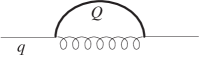
Figure 1: Mechanism generating quark masses through the exchange of a ETC particle.

We should also discuss dimension 5, 6, etc operators and why we need not include them in our analysis. Let us write some operators of dimension 5:

$$\bar{q}_{L}\hat{W}Uq_{R}+\mbox{h. c.},$$ (22)

$$\bar{q}_{L}U\hat{B}q_{R}+\mbox{h. c.},$$ (23)

$$\bar{q}_{L}\sigma^{\mu\nu}D^{\dagger}{}_{[\mu}D_{\nu]}Uq_{R}-\bar{q}_{L}\sigma^{\mu\nu}D_{[\nu}UD_{\mu]}q_{R}+\mbox{h. c.},$$ (24)

$$\bar{q}_{L}UD^{2}q_{R}+\mbox{h. c.},$$ (25)

$$\bar{q}_{L}D^{\dagger}_{\mu}U\tau^{3}U^{\dagger}(D^{\mu}U)q_{R}-\bar{q}_{L}U\tau^{3}U^{\dagger}(D^{\mu}U)D_{\mu}q_{R}+\mbox{h. c.};$$ (26)

$$\ldots$$

where we use the notation $\hat{W}\equiv{\rm i}g\sigma^{\mu\nu}W_{\mu\nu}$, $\hat{B}\equiv{\rm i}g^{\prime}\sigma^{\mu\nu}B_{\mu\nu}$. These are a few of a long list of about 25 operators, and this including only the ones contributing to the $ffZ$ vertex. All these operators are however chirality flipping and thus their contribution to the amplitude must be suppressed by one additional power of the fermion masses. This makes their study unnecessary at the present level of precision. Similar considerations apply to operators of dimensionality 6 or higher.

4 The effective theory of the Standard Model

In this section we shall obtain the values of the coefficients $\delta_{i}$ in the minimal Standard Model. The appropriate effective coefficients for the oblique corrections $a_{i}$ have been obtained previously by several authors[11, 12, 18]. Their values are

$$a_{0}=\frac{1}{16\pi^{2}}\frac{3}{8}\left(\frac{1}{\hat{\epsilon}}-\log\frac{M_{H}^{2}}{\mu^{2}}+\frac{5}{6}\right)$$ (27)

$$a_{1}=\frac{1}{16\pi^{2}}\frac{1}{12}\left(\frac{1}{\hat{\epsilon}}-\log\frac{M_{H}^{2}}{\mu^{2}}+\frac{5}{6}\right)$$ (28)

$$a_{8}=0.$$ (29)

where $1/\hat{\epsilon}\equiv 1/\epsilon-\gamma_{E}+\log 4\pi$. We use dimensional regularization with a spacetime dimension $4-2\epsilon$.

We begin by writing the Standard Model in terms of the non-linear variables $U$. The matrix

$${\cal M}=\sqrt{2}(\tilde{\Phi},\Phi),$$ (30)

constructed with the Higgs doublet, $\Phi$ and its conjugate, $\tilde{\Phi}\equiv{\rm i}\tau^{2}\Phi^{*}$, is rewritten in the form

$${\cal M}=(v+\rho)U,\qquad U^{-1}=U^{\dagger},$$ (31)

where $\rho$ describe the ‘radial’ excitations around the v.e.v. $v$. Integrating out the field $\rho$ produces an effective lagrangian of the form (1) with the values of the $a_{i}$ given above (as well as some other pieces not shown there). This functional integration also generates the vertex corrections (16).

We shall determine the $\delta_{i}$ by demanding that the renormalised one-particle irreducible Green functions (1PI), $\hat{\Gamma}$, are the same (up to some power in the external momenta and mass expansion) in both, the minimal Standard Model and the effective lagrangian. In other words, we require that

$$\Delta\hat{\Gamma}=0,$$ (32)

where throughout this section

$$\Delta\Gamma\equiv\Gamma_{{\rm SM}}-\Gamma_{{\rm eff}},$$ (33)

and the hat denotes renormalised quantities. This procedure is known as matching. It goes without saying that in doing so the same renormalization scheme must be used. The on-shell scheme is particularly well suited to perform the matching and will be used throughout this paper.

One only needs to worry about SM diagrams that are not present in the effective theory; namely, those containing the Higgs. The rest of the diagrams give exactly the same result, thus dropping from the matching. In contrast, the diagrams containing a Higgs propagator are described by local terms (such as ${\cal L}^{1}_{4}$ through ${\cal L}^{7}_{4}$) in the effective theory, they involve the coefficients $\delta_{i}$, and give rise to the Feynman rules collected in appendix B.

Let us first consider the fermion self-energies. There is only one 1PI diagram with a Higgs propagator (see figure 2).

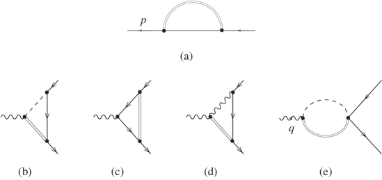
Figure 2: The diagrams relevant for the matching of the fermion self-energies and vertices (counterterm diagrams are not included). Double lines represent the Higgs, dashed lines the Goldstone bosons, and wiggly lines the gauge bosons.

A straightforward calculation gives

$$\Sigma^{f}_{{\rm SM}}=-{\frac{y_{f}^{2}}{16\pi^{2}}}\left\{/\kern-5.69054ptp\left[{\frac{1}{2}}{1\over\hat{\epsilon}}-{\frac{1}{2}}\log{\frac{M_{H}^{2}}{\mu^{2}}}+{\frac{1}{4}}\right]+m_{f}\left[{1\over\hat{\epsilon}}-\log{\frac{M_{H}^{2}}{\mu^{2}}}+1\right]\right\}.$$ (34)

$\Delta\Sigma^{f}$ can be computed by subtracting (121), (122) from (34).

Next, we have to renormalise the fermion self-energies. We introduce the following notation

$$\Delta Z\equiv Z_{{\rm SM}}-Z_{{\rm eff}}=\delta Z_{{\rm SM}}-\delta Z_{{\rm eff}},$$ (35)

where $Z_{{\rm SM}}$ ($Z_{{\rm eff}}$) stands for any renormalization constant of the SM (effective theory). To compute $\Delta\hat{\Sigma}^{f}$, we simply add to $\Delta\Sigma^{f}$ the counterterm diagram (150) with the replacements $\delta Z^{f}_{V,A}\to\Delta Z^{f}_{V,A}$ and $\delta m_{f}\to\Delta m_{f}$. This, of course, amounts to eqs. (157), (158) and (159) with the same replacements. From (160), (161) and (162) (which also hold for $\Delta Z$, $\Delta m$ and $\Delta\Sigma$) one can express $\Delta Z^{f}_{V,A}$ and $\Delta m_{f}/m_{f}$ in terms of the bare fermion self-energies and finally obtain $\Delta\hat{\Sigma}^{f}$. The result is

$$\Delta\hat{\Sigma}^{d}_{A,V,S} = 0$$ (36)

$$\Delta\hat{\Sigma}^{u}_{A} = 0$$ (37)

$$\Delta\hat{\Sigma}^{u}_{V,S} = 4\delta_{7}-{\frac{1}{16\pi^{2}}}{\frac{y_{u}^{2}-y_{d}^{2}}{2}}\left[{1\over\hat{\epsilon}}-\log{\frac{M_{H}^{2}}{\mu^{2}}}+{\frac{1}{2}}\right].$$ (38)

We see from (38) that the matching conditions, $\Delta\hat{\Sigma}^{u}_{V,S}=0$, imply

$$\delta_{7}={\frac{1}{16\pi^{2}}}{\frac{y_{u}^{2}-y_{d}^{2}}{8}}\left[{1\over\hat{\epsilon}}-\log{\frac{M_{H}^{2}}{\mu^{2}}}+{\frac{1}{2}}\right].$$ (39)

The other matchings are satisfied automatically and do not give any information.

Let us consider the vertex $ffZ$. The relevant diagrams are shown in figure 2 (diagrams b–e). We shall only collect the contributions proportional to $\gamma_{\mu}$ and $\gamma_{\mu}\gamma_{5}$. The result is

$$\Gamma_{\mu}^{ffZ}=-{\frac{{\rm i}}{16\pi^{2}}}{\frac{y_{f}^{2}}{2}}\gamma_{\mu}\left\{v_{f}\left({1\over\hat{\epsilon}}-\log{\frac{M_{H}^{2}}{\mu^{2}}}+{\frac{1}{2}}\right)-3a_{f}\,\gamma_{5}\left({1\over\hat{\epsilon}}-\log{\frac{M_{H}^{2}}{\mu^{2}}}+{\frac{11}{6}}\right)\right\}.$$ (40)

By subtracting the diagrams (116) and (117) from $\Gamma_{\mu}^{ffZ}$ one gets $\Delta\Gamma_{\mu}^{ffZ}$. Renormalization requires that we add the counterterm diagram (151) where, again, $\delta Z\to\Delta Z$. One can check that both $\Delta Z^{Z}_{1}-\Delta Z^{Z}_{2}$ and $\Delta Z^{Z\gamma}_{1}-\Delta Z^{Z\gamma}_{2}$ are proportional to $\Delta\Sigma_{Z\gamma}(0)$, which turns out to be zero. Hence the only relevant renormalization constants are $\Delta Z_{V}^{f}$ and $\Delta Z_{A}^{f}$. These renormalization constant have already been determined. One obtains for $\Delta\hat{\Gamma}^{ffZ}_{\mu}$ the result

$$\Delta\hat{\Gamma}^{ddZ}_{\mu} = -{\frac{{\rm i}e}{2s_{W}c_{W}}}\gamma_{\mu}\left\{\left[{\displaystyle{1\over 2}}(\delta_{1}-\delta_{4}-\delta_{2}-\delta_{6})+\delta_{3}+\delta_{5}\right]\phantom{\left[{1\over\hat{\epsilon}}-\log{\frac{M_{H}^{2}}{\mu^{2}}}+{\frac{5}{2}}\right]}\right.$$ (41)

$$- \left.\gamma_{5}\left[{\frac{1}{16\pi^{2}}}{\frac{y_{d}^{2}}{2}}\left({1\over\hat{\epsilon}}-\log{\frac{M_{H}^{2}}{\mu^{2}}}+{\frac{5}{2}}\right)+{\displaystyle{1\over 2}}(\delta_{1}-\delta_{4}+\delta_{2}+\delta_{6})+\delta_{3}-\delta_{5}\right]\right\}$$

$$\Delta\hat{\Gamma}^{uuZ}_{\mu} = -{\frac{{\rm i}e}{2s_{W}c_{W}}}\gamma_{\mu}\left\{\left[{\displaystyle{1\over 2}}(\delta_{1}-\delta_{4}-\delta_{2}-\delta_{6})-\delta_{3}-\delta_{5}\right]\phantom{\left[{1\over\hat{\epsilon}}-\log{\frac{M_{H}^{2}}{\mu^{2}}}+{\frac{5}{2}}\right]}\right.$$ (42)

$$- \left.\gamma_{5}\left[-{\frac{1}{16\pi^{2}}}{\frac{y_{u}^{2}}{2}}\left({1\over\hat{\epsilon}}-\log{\frac{M_{H}^{2}}{\mu^{2}}}+{\frac{5}{2}}\right)-{\displaystyle{1\over 2}}(\delta_{1}-\delta_{4}+\delta_{2}+\delta_{6})+\delta_{3}-\delta_{5}\right]\right\},$$

where use has been made of eq. (39). The matching condition, $\Delta\hat{\Gamma}^{ffZ}_{\mu}=0$ implies

$$\delta_{1}-\delta_{4} = -{\frac{1}{16\pi^{2}}}{\frac{y_{u}^{2}+y_{d}^{2}}{4}}\left({1\over\hat{\epsilon}}-\log{\frac{M_{H}^{2}}{\mu^{2}}}+{\frac{5}{2}}\right)$$ (43)

$$\delta_{2}+\delta_{6} = -{\frac{1}{16\pi^{2}}}{\frac{y_{u}^{2}+y_{d}^{2}}{4}}\left({1\over\hat{\epsilon}}-\log{\frac{M_{H}^{2}}{\mu^{2}}}+{\frac{5}{2}}\right)$$ (44)

$$\delta_{3} = \phantom{-}{\frac{1}{16\pi^{2}}}{\frac{y_{u}^{2}-y_{d}^{2}}{4}}\left({1\over\hat{\epsilon}}-\log{\frac{M_{H}^{2}}{\mu^{2}}}+{\frac{5}{2}}\right)$$ (45)

$$\delta_{5} = -{\frac{1}{16\pi^{2}}}{\frac{y_{u}^{2}-y_{d}^{2}}{4}}\left({1\over\hat{\epsilon}}-\log{\frac{M_{H}^{2}}{\mu^{2}}}+{\frac{5}{2}}\right).$$ (46)

To determine completely the $\delta_{i}$ coefficients we need to consider the vertex $udW$. The relevant diagrams are analogous to those of figure 2. A straightforward calculation gives

$$\Delta\hat{\Gamma}_{\mu}^{udW} = {\frac{{\rm i}e}{4\sqrt{2}s_{W}}}\;\gamma_{\mu}\left\{\left[{\frac{y_{u}y_{d}}{16\pi^{2}}}\left({1\over\hat{\epsilon}}-\log{\frac{M_{H}^{2}}{\mu^{2}}}+{\frac{5}{2}}\right)+2\delta_{2}-2\delta_{6}\right](1+\gamma_{5})\right.$$ (47)

$$\left.-\left[{\frac{y_{u}^{2}+y_{d}^{2}}{16\pi^{2}}}{\displaystyle{1\over 2}}\left({1\over\hat{\epsilon}}-\log{\frac{M_{H}^{2}}{\mu^{2}}}+{\frac{5}{2}}\right)+2\delta_{1}+2\delta_{4}\right](1-\gamma_{5})\right\}.$$

The matching condition $\Delta\hat{\Gamma}_{\mu}^{udW}=0$ amounts to the following set of equations

$$\delta_{2}-\delta_{6} = -{\frac{1}{16\pi^{2}}}{\frac{y_{u}y_{d}}{2}}\left({1\over\hat{\epsilon}}-\log{\frac{M_{H}^{2}}{\mu^{2}}}+{\frac{5}{2}}\right)$$ (48)

$$\delta_{1}+\delta_{4} = -{\frac{1}{16\pi^{2}}}{\frac{y_{u}^{2}+y_{d}^{2}}{4}}\left({1\over\hat{\epsilon}}-\log{\frac{M_{H}^{2}}{\mu^{2}}}+{\frac{5}{2}}\right)$$ (49)

Combining these equations with eqs. (43, 44) we finally get

$$\delta_{1} = -{\frac{1}{16\pi^{2}}}{\frac{y_{u}^{2}+y_{d}^{2}}{4}}\left({1\over\hat{\epsilon}}-\log{\frac{M_{H}^{2}}{\mu^{2}}}+{\frac{5}{2}}\right)$$ (50)

$$\delta_{2} = -{\frac{1}{16\pi^{2}}}{\frac{(y_{u}+y_{d})^{2}}{8}}\left({1\over\hat{\epsilon}}-\log{\frac{M_{H}^{2}}{\mu^{2}}}+{\frac{5}{2}}\right)$$ (51)

$$\delta_{4} = 0$$ (52)

$$\delta_{6} = -{\frac{1}{16\pi^{2}}}{\frac{(y_{u}-y_{d})^{2}}{8}}\left({1\over\hat{\epsilon}}-\log{\frac{M_{H}^{2}}{\mu^{2}}}+{\frac{5}{2}}\right)$$ (53)

This, along with eqs. (45, 46) and eq. (39), is our final answer. These results coincide, where the comparison is possible, with those obtained in [19] by functional methods. It is interesting to note that it has not been necessary to consider the matching of the vertex $ff\gamma$.

We shall show explicitly that $\delta_{7}$ drops from the $S$ matrix element corresponding to $Z\to f\bar{f}$. It is well known that the renormalised $u$-fermion self-energy has residue $1+\delta_{\rm res}$, where $\delta_{\rm res}$ in given in eq. (163) of appendix D. Therefore, in order to evaluate $S$-matrix elements involving external $u$ lines at one-loop, one has to multiply the corresponding amputated Green functions by a factor $1+n\,\delta_{\rm res}/2$, where $n$ is the number on external $u$-lines (in the case under consideration $n=2$). One can check that when this factor is taken into account, the $\delta_{7}$ appearing in the renormalised S-matrix vertex are cancelled.

We notice that $\delta_{1}$ and $\delta_{2}$ indeed correspond to custodially preserving operators, while $\delta_{3}$ to $\delta_{6}$ do not. All these coefficients (just as $a_{0}$, $a_{1}$ and $a_{8}$) are ultraviolet divergent. This is so because the Higgs particle is an essential ingredient to guarantee the renormalizability of the Standard Model. Once this is removed, the usual renormalization process (e.g. the on-shell scheme) is not enough to render all “renormalised” Green functions finite. This is why the bare coefficients of the effective lagrangian (which contribute to the renormalised Green functions either directly or via counterterms) have to be proportional to $1/\epsilon$ to cancel the new divergences. The coefficients of the effective lagrangian are manifestly gauge invariant.

What is the value of these coefficients in other theories with elementary scalars and Higgs-like mechanism? This issue has been discussed in some detail in [20] in the context of the two-Higgs doublet model, but it can actually be extended to supersymmetric theories (provided of course scalars other than the CP-even Higgs can be made heavy enough, see e.g. [21]). It was argued there that non-decoupling effects are exactly the same as in the minimal Standard Model, including the constant non-logarithmic piece. Since the $\delta_{i}$ coefficients contain all the non-decoupling effects associated to the Higgs particle at the first non-trivial order in the momentum or mass expansion, the low energy effective theory will be exactly the same.

5 Observables

The decay width of $Z\rightarrow f\bar{f}$ is described by

$$\Gamma_{f}\equiv\Gamma\left(Z\rightarrow f\bar{f}\right)=4n_{c}\Gamma_{0}\left[\left(g_{V}^{f}\right)^{2}R_{V}^{f}+\left(g_{A}^{f}\right)^{2}R_{A}^{f}\right],$$ (54)

where $g_{V}^{f}$ and $g_{A}^{f}$ are the effective electroweak couplings as defined in [22] and $n_{c}$ is the number of colours of fermion $f$. The radiation factors $R_{V}^{f}$ and $R_{A}^{f}$ describe the final state QED and QCD interactions [23]. For a charged lepton we have

$$R_{V}^{l} = 1+\frac{3\bar{\alpha}}{4\pi}+{\cal O}\left(\bar{\alpha}^{2},\left(\frac{m_{l}}{M_{Z}}\right)^{4}\right),$$

$$R_{A}^{l} = 1+\frac{3\bar{\alpha}}{4\pi}-6\left(\frac{m_{l}}{M_{Z}}\right)^{2}+{\cal O}\left(\bar{\alpha}^{2},\left(\frac{m_{l}}{M_{Z}}\right)^{4}\right),$$

where $\bar{\alpha}$ is the electromagnetic coupling constant at the scale $M_{Z}$ and $m_{l}$ is the final state lepton mass

The tree-level width $\Gamma_{0}$ is given by

$$\Gamma_{0}=\frac{G_{\mu}M_{Z}^{3}}{24\sqrt{2}\pi}.$$ (55)

If we define

$$\rho_{f}\equiv 4\left(g_{A}^{f}\right)^{2},$$ (56)

$$\bar{s}_{W}^{2}\equiv\frac{I_{f}^{3}}{2Q_{f}}\left(1-\frac{g_{V}^{f}}{g_{A}^{f}}\right),$$ (57)

we can write

$$\Gamma_{f}=n_{c}\Gamma_{0}\rho_{f}\left[4\left(I_{f}^{3}-2Q_{f}\bar{s}_{W}^{2}\right)^{2}R_{V}^{f}+R_{A}^{f}\right].$$ (58)

Other quantities which are often used are $\Delta\rho_{f}$, defined through

$$\rho_{f}\equiv\frac{1}{1-\Delta\rho_{f}},$$ (59)

the forward-backward asymmetry $A_{FB}^{f}$

$$A_{FB}^{f}=\frac{3}{4}A^{e}A^{f},$$ (60)

and $R_{b}$

$$R_{b}=\frac{\Gamma_{b}}{\Gamma_{h}},$$ (61)

where

$$A^{f}\equiv\frac{2g_{V}^{f}g_{A}^{f}}{\left(g_{A}^{f}\right)^{2}+\left(g_{V}^{f}\right)^{2}},$$

and $\Gamma_{b}$, $\Gamma_{h}$ are the b-partial width and total hadronic width, respectively (each of them, in turn, can be expressed in terms of the appropriate effective couplings). As we see, nearly all of $Z$ physics can be described in terms of $g_{A}^{f}$ and $g_{V}^{f}$. The box contributions to the process $e^{+}e^{-}\rightarrow f\bar{f}$ are not included in the analysis because they are negligible and they cannot be incorporated as contributions to effective electroweak neutral current couplings anyway.

We shall generically denote these effective couplings by $g^{f}$. If we express the value they take in the Standard Model by $g^{f\left(SM\right)}$, we can write a perturbative expansion for them in the following way

$$g^{f\left({\rm SM}\right)}=g^{f\left(0\right)}+g^{f\left(2\right)}+\bar{g}^{f}({a}^{\rm SM})+\hat{g}^{f}({\delta}^{\rm SM}),$$ (62)

where $g^{f\left(0\right)}$ are the tree-level expressions for these form factors, $g^{f\left(2\right)}$ are the one-loop contributions which do not contain any Higgs particle as internal line in the Feynman graphs. In the effective lagrangian language they are generated by the quantum corrections computed by operators such as (6) or the first operator on the r.h.s. of (1). On the other hand, the Feynman diagrams containing the Higgs particle contribute to $g^{f\left(SM\right)}$ in a twofold way. One is via the ${\cal O}(p^{2})$ and ${\cal O}(p^{4})$ Longhitano effective operators (1) which depend on the $a_{i}$ coefficients, which are Higgs-mass dependent, and thus give a Higgs-dependent oblique correction to $g^{f\left(SM\right)}$, which is denoted by $\bar{g}^{f}$. The other one is via genuine vertex corrections which depend on the $\delta_{i}$. This contribution is denoted by $\hat{g}^{f}$.

The tree-level value for the form factors are

$$g_{V}^{f\left(0\right)}=I_{f}^{3}-2s_{W}^{2}Q_{f},\qquad g_{A}^{f\left(0\right)}=I_{f}^{3}.$$ (63)

In a theory X, different from the minimal Standard Model, the effective form factors will take values $g^{f\left({\rm X}\right)}$, where

$$g^{f\left({\rm X}\right)}=g^{f\left(0\right)}+g^{f\left(2\right)}+\bar{g}^{f}({a}^{\rm X})+\hat{g}^{f}({\delta}^{\rm X}),$$ (64)

and the ${a}^{\rm X}$ and ${\delta}^{\rm X}$ are effective coefficients corresponding to theory X.

Within one-loop accuracy in the symmetry breaking sector (but with arbitrary precision elsewhere), $\bar{g}^{f}$ and $\hat{g}^{f}$ are linear functions of their arguments and thus we have

$$g^{f\left({\rm X}\right)}=g^{f\left({\rm SM}\right)}+\bar{g}^{f}({a}^{\rm X}-{a}^{\rm SM})+\hat{g}^{f}({\delta}^{\rm X}-{\delta}^{\rm SM}).$$ (65)

The expression for $\bar{g}^{f}$ in terms of $a_{i}$ was already given in (4) and (5). On the other hand from appendix B we learn that

$$\hat{g}_{V}^{f}\left(\delta_{1},\cdots,\delta_{6}\right)=I_{f}^{3}\left(\delta_{1}-\delta_{4}-\delta_{2}-\delta_{6}\right)-\delta_{3}-\delta_{5},$$ (66)

$$\hat{g}_{A}^{f}\left(\delta_{1},\cdots,\delta_{6}\right)=I_{f}^{3}\left(\delta_{1}-\delta_{4}+\delta_{2}+\delta_{6}\right)-\delta_{3}+\delta_{5},$$ (67)

In the minimal Standard Model all the Higgs dependence at the one loop level (which is the level of accuracy assumed here) is logarithmic and is contained in the $a_{i}$ and $\delta_{i}$ coefficients. Therefore one can easily construct linear combinations of observables where the leading Higgs dependence cancels. These combinations allow for a test of the minimal Standard Model independent of the actual value of the Higgs mass.

Let us now review the comparison with current electroweak data for theories with dynamical symmetry breaking. Some confusion seem to exist on this point so let us try to analyze this issue critically.

A first difficulty arises from the fact that at the $M_{Z}$ scale perturbation theory is not valid in theories with dynamical breaking and the contribution from the symmetry breaking sector must be estimated in the framework of the effective theory, which is non-linear and non-renormalizable. Observables will depend on some subtraction scale. (Estimates based on dispersion relations and resonance saturation amount, in practice, to the same, provided that due attention is paid to the scale dependence introduced by the subtraction in the dispersion relation.)

A somewhat related problem is that, when making use of the variables $S,T$ and $U$[13], or $\epsilon_{1},\epsilon_{2}$ and $\epsilon_{3}$[24], one often sees in the literature bounds on possible “new physics” in the symmetry breaking sector without actually removing the contribution from the Standard Model higgs that the “new physics” is supposed to replace (this is not the case e.g. in [13] where this issue is discussed with some care). Unless the contribution from the “new physics” is enormous, this is a flagrant case of double counting, but it is easy to understand why this mistake is made: removing the Higgs makes the Standard Model non-renormalizable and the observables of the Standard Model without the Higgs depend on some arbitrary subtraction scale.

In fact the two sources of arbitrary subtraction scales (the one originating from the removal of the Higgs and the one from the effective action treatment) are one an the same and the problem can be dealt with the help of the coefficients of higher dimensional operators in the effective theory (i.e. the $a_{i}$ and $\delta_{i}$). The dependence on the unknown subtraction scale is absorbed in the coefficients of higher dimensional operators and traded by the scale of the “new physics”. Combinations of observables can be built where this scale (and the associated renormalization ambiguities) drops. These combinations allow for a test of the “new physics” independently of the actual value of its characteristic scale. In fact they are the same combinations of observables where the Higgs dependence drops in the minimal Standard Model.

A third difficulty in making a fair comparison of models of dynamical symmetry breaking with experiment lies in the vertex corrections. If we analyze the lepton effective couplings $g_{A}^{l}$ and $g_{V}^{l}$, the minimal Standard Model predicts very small vertex corrections arising from the symmetry breaking sector anyway and it is consistent to ignore them and concentrate in the oblique corrections. However, this is not the situation in dynamical symmetry breaking models. We will see in the next sections that for the second and third generation vertex corrections can be sizeable. Thus if we want to compare experiment to oblique corrections in models of dynamical breaking we have to concentrate on electron couplings only.

Figure 3: The $1-\sigma$ experimental region in the $g_{A}^{e}-g_{V}^{e}$ plane. The Standard Model predictions as a function of $m_{t}$ ($170.6\leq m_{t}\leq 180.6$ GeV) and $M_{H}$ ($70\leq M_{H}\leq 1000$ GeV) are shown (the middle line corresponds to the central value $m_{t}=175.6$ GeV). The predictions of a QCD-lke technicolor theory with $n_{TC}n_{D}=8$ and degenerate technifermion masses are shown as straight lines (only oblique corrections are included). One moves along the straight lines by changing the scale $\Lambda$. The three lines correspond to the extreme and central values for $m_{t}$. Recall that the precise location anywhere on the straight lines (which definitely do intersect the $1-\sigma$ region) depends on the renormalization procedure and thus is not predictable within the non-renormalizable effective theory. In addition the technicolor prediction should be considered accurate only at the 15% level due to the theoretical uncertainties discussed in the text (this error is at any rate smaller than the one associated to the uncertainty in $\Lambda$). Notice that the oblique corrections, in the case of degenerate masses, are independent of the value of the technifermion mass. Assuming universality of the vertex corrections reduces the error bars by about a factor one-half and leaves technicolor predictions outside the $1-\sigma$ region.

In figure 3 we see the prediction of the minimal Standard Model for $170.6<m_{t}<180.6$ GeV and $70<M_{H}<1000$ GeV including the leading two-loop corrections[23], falling nicely within the experimental $1-\sigma$ region for the electron effective couplings. In this and in subsequent plots we present the data form the combined four LEP experiments only. What is the actual prediction for a theory with dynamical symmetry breaking? The straight solid lines correspond to the prediction of a QCD-like technicolor model with $n_{TC}=2$ and $n_{D}=4$ (a one-generation model) in the case where all technifermion masses are assumed to be equal (we follow [9], see [25] for related work) allowing the same variation for the top mass as in the Standard Model. We do not take into account here the contribution of potentially present pseudo Goldstone bosons, assuming that they can be made heavy enough. The corresponding values for the $a_{i}$ coefficients in such a model are given in appendix E and are derived using chiral quark model techniques and chiral perturbation theory. They are scale dependent in such a way as to make observables finite and unambiguous, but of course observables depend in general on the scale of “new physics” $\Lambda$.

We move along the straight lines by changing the scale $\Lambda$. It would appear at first sight that one needs to go to unacceptably low values of the new scale to actually penetrate the $1-\sigma$ region, something which looks unpleasant at first sight (we have plotted the part of the line for $100\leq\Lambda\leq 1500$ GeV), as one expects $\Lambda\sim\Lambda_{\chi}$. In fact this is not necessarily so. There is no real prediction of the effective theory along the straight lines, because only combinations which are $\Lambda$-independent are predictable. As for the location not along the line, but of the line itself it is in principle calculable in the effective theory, but of course subject to the uncertainties of the model one relies upon, since we are dealing with a strongly coupled theory. (We shall use chiral quark model estimates in this paper as we believe that they are quite reliable for QCD-like theories, see the discussion below.)

If we allow for a splitting in the technifermion masses the comparison with experiment improves very slightly. The values of the effective lagrangian coefficients relevant for the oblique corrections in the case of unequal masses are also given in appendix E. Since $a_{1}$ is independent of the technifermion dynamically generated masses anyway, the dependence is fully contained in $a_{0}$ (the parameter $T$ of Peskin and Takeuchi[13]) and $a_{8}$ (the parameter $U$). This is shown in figure 4. We assume that the splitting is the same for all doublets, which is not necessarily true.

If other representations of the $SU(2)_{L}\times SU(3)_{c}$ gauge group are used, the oblique corrections have to be modified in the form prescribed in section 8. Larger group theoretical factors lead to larger oblique corrections and, from this point of view, the restriction to weak doublets and colour singlets or triplets is natural.

Let us close this section by justifying the use of chiral quark model techniques, trying to assess the errors involved, and at the same time emphasizing the importance of having the scale dependence under control. A parameter like $a_{1}$ (or $S$ in the notation of Peskin and Takeuchi[13]) contains information about the long-distance properties of a strongly coupled theory. In fact, $a_{1}$ is nothing but the familiar $L_{10}$ parameter of the strong chiral lagrangian of Gasser and Leutwyler[26] translated to the electroweak sector. This strong interaction parameter can be measured and it is found to be $L_{10}=(-5.6\pm 0.3)\times 10^{-3}$ (at the $\mu=M_{\eta}$ scale, which is just the conventional reference value and plays no specific role in the Standard Model.) This is almost twice the value predicted by the chiral quark model[27, 28] ($L_{10}=-1/32\pi^{2}$), which is the estimate plotted in figure 3. Does this mean that the chiral quark model grossly underestimates this observable? Not at all. Chiral perturbation theory predicts the running of $L_{10}$. It is given by

$$L_{10}(\mu)=L_{10}(M_{\eta})+\frac{1}{128\pi^{2}}\log\frac{\mu^{2}}{M_{\eta}^{2}}.$$ (68)

According to our current understanding (see e.g. [29]), the chiral quark model gives the value of the chiral coefficients at the chiral symmetry breaking scale ($4\pi f_{\pi}$ in QCD, $\Lambda_{\chi}$ in the electroweak theory). Then the coefficient $L_{10}$ (or $a_{1}$ for that matter) predicted within the chiral quark model agrees with QCD at the 10% level.

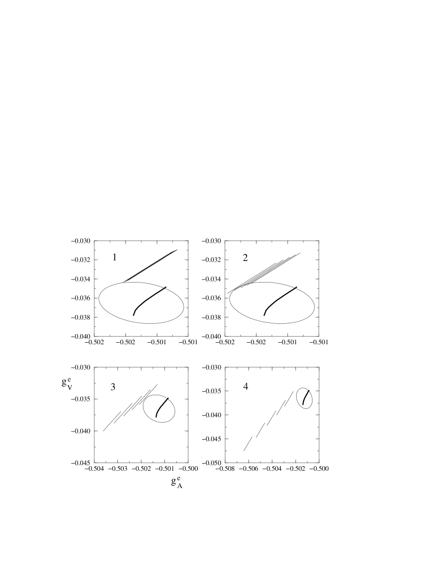
Figure 4: The effect of isospin breaking in the oblique corrections in QCD-like technicolor theories. The $1-\sigma$ region for the $g_{A}^{e}-g_{V}^{e}$ couplings and the SM prediction (for $m_{t}=175.6$ GeV, and $70\leq M_{H}\leq 1000$ GeV) are shown. The different straight lines correspond to setting the technifermion masses in each doublet ($m_{1}$, $m_{2}$) to the value $m_{2}=$ 250, 300, 350, 400 and 450 GeV (larger masses are the ones deviating more from the SM predictions), and $m_{1}=1.05m_{2}$ (plot 1), $m_{1}=1.1m_{2}$ (plot 2), $m_{1}=1.2m_{2}$ (plot 3), and $m_{1}=1.3m_{2}$ (plot 4). The results are invariant under the exchange of $m_{1}$ and $m_{2}$. As in figure 3 the prediction of the effective theory is the whole straight line and not any particular point on it, as we move along the line by varying the unknown scale $\Lambda$. Clearly isospin breakings larger than 20 % give very poor agreement with the data, even for low values of the dynamically generated mass.

Let us now turn to the issue of vertex corrections in theories with dynamical symmetry breaking and the determination of the coefficients $\delta_{i}$ which are, after all, the focal point of this work.

6 New physics and four-fermion operators

In order to have a picture in our mind, let us assume that at sufficiently high energies the symmetry breaking sector can be described by some renormalizable theory, perhaps a non-abelian gauge theory. By some unspecified mechanism some of the carriers of the new interaction acquire a mass. Let us generically denote this mass by $M$. One type of models that comes immediately to mind is the extended technicolor scenario. $M$ would then be the mass of the ETC bosons. Let us try, however, not to adhere to any specific mechanism or model.

Below the scale $M$ we shall describe our underlying theory by four-fermion operators. This is a convenient way of parametrizing the new physics below $M$ without needing to commit oneself to a particular model. Of course the number of all possible four-fermion operators is enormous and one may think that any predictive power is lost. This is not so because of two reasons: a) The size of the coefficients of the four fermion operators is not arbitrary. They are constrained by the fact that at scale $M$ they are given by

$$-\xi_{\rm CG}\frac{G^{2}}{M^{2}}$$ (69)

where $\xi_{\rm CG}$ is built out of Clebsch-Gordan factors and $G$ a gauge coupling constant, assumed perturbative of ${\cal O}(1)$ at the scale $M$. The $\xi_{\rm CG}$ being essentially group-theoretical factors are probably of similar size for all three generations, although not necessarily identical as this would assume a particular style of embedding the different generations into the large ETC (for instance) group. Notice that for four-fermion operators of the form ${\bf J}\cdot{\bf J}^{\dagger}$, where ${\bf J}$ is some fermion bilinear, $\xi_{\rm CG}$ has a well defined sign, but this is not so for other operators. b) It turns out that only a relatively small number of combinations of these coefficients do actually appear in physical observables at low energies.

Matching to the fundamental physical theory at $\mu=M$ fixes the value of the coupling constants accompanying the four-fermion operators to the value (69). In addition contact terms, i.e. non-zero values for the effective coupling constants $\delta_{i}$, are generally speaking required in order for the fundamental and four-fermion theories to match. These will later evolve under the renormalization group due to the presence of the four-fermion interactions. Because we expect that $M\gg\Lambda_{\chi}$, the $\delta_{i}$ will be typically logarithmically enhanced. Notice that there is no guarantee that this is the case for the third generation, as we will later discuss. In this case the TC and ETC dynamics would be tangled up (which for most models is strongly disfavoured by the constraints on oblique corrections). For the first and second generation, however, the logarithmic enhancement of the $\delta_{i}$ is a potentially large correction and it actually makes the treatment of a fundamental theory via four-fermion operators largely independent of the particular details of specific models, as we will see.

Let us now get back to four-fermion operators and proceed to a general classification. A first observation is that, while in the bosonic sector custodial symmetry is just broken by the small $U(1)_{Y}$ gauge interactions, which is relatively small, in the matter sector the breaking is not that small. We thus have to assume that whatever underlying new physics is present at scale $M$ it gives rise both to custodially preserving and custodially non-preserving four-fermion operators with coefficients of similar strength. Obvious requirements are hermiticity, Lorentz invariance and $SU(3)_{c}\times SU(2)_{L}\times U(1)_{Y}$ symmetry. Neither $C$ nor $P$ invariance are imposed, but invariance under $CP$ is assumed.

We are interested in $d=6$ four-fermion operators constructed with two ordinary fermions (either leptons or quarks), denoted by $q_{L}$, $q_{R}$, and two fermions $Q^{A}_{L}$, $Q^{A}_{R}$. Typically $A$ will be the technicolor index and the $Q_{L}$, $Q_{R}$ will therefore be techniquarks and technileptons, but we may be as well interested in the case where the $Q$ may be ordinary fermions. In this case the index $A$ drops (in our subsequent formulae this will correspond to taking $n_{TC}=1$). We shall not write the index $A$ hereafter for simplicity, but this degree of freedom is explicitly taken into account in our results.

As we already mention we shall discuss in detail the case where the additional fermions fall into ordinary representations of $SU(2)_{L}\times SU(3)_{c}$ and will discuss other representations later. The fields $Q_{L}$ will therefore transform as $SU(2)_{L}$ doublets and we shall group the right-handed fields $Q_{R}$ into doublets as well, but then include suitable insertions of $\tau^{3}$ to consider custodially breaking operators. In order to determine the low energy remnants of all these four-fermion operators (i.e. the coefficients $\delta_{i}$) it is enough to know their couplings to $SU(2)_{L}$ and no further assumptions about their electric charges (or hypercharges) are needed. Of course, since the $Q_{L}$, $Q_{R}$ couple to the electroweak gauge bosons they must not lead to new anomalies. The simplest possibility is to assume they reproduce the quantum numbers of one family of quarks and leptons (that is, a total of four doublets $n_{D}=4$), but other possibilities exist (for instance $n_{D}=1$ is also possible[31], although this model presents a global $SU(2)_{L}$ anomaly).

We shall first be concerned with the $Q_{L}$, $Q_{R}$ fields belonging to the representation ${\bf 3}$ of $SU(3)_{c}$ and afterwards, focus in the simpler case where the $Q_{L}$, $Q_{R}$ are colour singlet (technileptons). Coloured $Q_{L}$, $Q_{R}$ fermions can couple to ordinary quarks and leptons either via the exchange of a colour singlet or of a colour octet. In addition the exchanged particle can be either an $SU(2)_{L}$ triplet or a singlet, thus leading to a large number of possible four-fermion operators. More important for our purposes will be whether they flip or not the chirality. We use Fierz rearrangements in order to write the four-fermion operators as product of either two colour singlet or two colour octet currents. A complete list is presented in table 1 and table 2 for the chirality preserving and chirality flipping operators, respectively.

$L^{2}=(\bar{Q}_{L}\gamma_{\mu}Q_{L})(\bar{q}_{L}\gamma^{\mu}q_{L})$
$R^{2}=(\bar{Q}_{R}\gamma_{\mu}Q_{R})(\bar{q}_{R}\gamma^{\mu}q_{R})$	$R_{3}R=(\bar{Q}_{R}\gamma_{\mu}\tau^{3}Q_{R})(\bar{q}_{R}\gamma^{\mu}q_{R})$
	$RR_{3}=(\bar{Q}_{R}\gamma_{\mu}Q_{R})(\bar{q}_{R}\gamma^{\mu}\tau^{3}q_{R})$
	$R_{3}^{2}=(\bar{Q}_{R}\gamma_{\mu}\tau^{3}Q_{R})(\bar{q}_{R}\gamma^{\mu}\tau^{3}q_{R})$
$RL=(\bar{Q}_{R}\gamma_{\mu}Q_{R})(\bar{q}_{L}\gamma^{\mu}q_{L})$	$R_{3}L=(\bar{Q}_{R}\gamma_{\mu}\tau^{3}Q_{R})(\bar{q}_{L}\gamma^{\mu}q_{L})$
$LR=(\bar{Q}_{L}\gamma_{\mu}Q_{L})(\bar{q}_{R}\gamma^{\mu}q_{R})$	$LR_{3}=(\bar{Q}_{L}\gamma_{\mu}Q_{L})(\bar{q}_{R}\gamma^{\mu}\tau^{3}q_{R})$
$rl=(\bar{Q}_{R}\gamma_{\mu}\vec{\lambda}Q_{R})\cdot(\bar{q}_{L}\gamma^{\mu}\vec{\lambda}q_{L})$	$r_{3}l=(\bar{Q}_{R}\gamma_{\mu}\vec{\lambda}\tau^{3}Q_{R})\cdot(\bar{q}_{L}\gamma^{\mu}\vec{\lambda}q_{L})$
$lr=(\bar{Q}_{L}\gamma_{\mu}\vec{\lambda}Q_{L})\cdot(\bar{q}_{R}\gamma^{\mu}\vec{\lambda}q_{R})$	$lr_{3}=(\bar{Q}_{L}\gamma_{\mu}\vec{\lambda}Q_{L})\cdot(\bar{q}_{R}\gamma^{\mu}\vec{\lambda}\tau^{3}q_{R})$
$(\bar{Q}_{L}\gamma_{\mu}q_{L})(\bar{q}_{L}\gamma^{\mu}Q_{L})$
$(\bar{Q}_{R}\gamma_{\mu}q_{R})(\bar{q}_{R}\gamma^{\mu}Q_{R})$	$(\bar{Q}_{R}\gamma_{\mu}\tau^{3}q_{R})(\bar{q}_{R}\gamma^{\mu}Q_{R})+(\bar{Q}_{R}\gamma_{\mu}q_{R})(\bar{q}_{R}\gamma^{\mu}\tau^{3}Q_{R})$
	$(\bar{Q}_{R}\gamma_{\mu}\tau^{3}q_{R})(\bar{q}_{R}\gamma^{\mu}\tau^{3}Q_{R})$
$(\bar{Q}_{L}^{i}\gamma_{\mu}Q^{j}_{L})(\bar{q}_{L}^{j}\gamma^{\mu}q_{L}^{i})$
$(\bar{Q}_{R}^{i}\gamma_{\mu}Q^{j}_{R})(\bar{q}_{R}^{j}\gamma^{\mu}q_{R}^{i})$
$(\bar{Q}_{L}^{i}\gamma_{\mu}q_{L}^{j})(\bar{q}_{L}^{j}\gamma^{\mu}Q_{L}^{i})$
$(\bar{Q}_{R}^{i}\gamma_{\mu}q_{R}^{j})(\bar{q}_{R}^{j}\gamma^{\mu}Q_{R}^{i})$	$(\bar{Q}_{R}^{i}\gamma_{\mu}q_{R}^{j})(\bar{q}_{R}^{j}\gamma^{\mu}[\tau^{3}Q_{R}]^{i})$

Table 1: Four-fermion operators which do not change the fermion chirality. The first (second) column contains the custodially preserving (breaking) operators.

$(\bar{Q}_{L}\gamma^{\mu}q_{L})(\bar{q}_{R}\gamma_{\mu}Q_{R})$	$(\bar{Q}_{L}\gamma^{\mu}q_{L})(\bar{q}_{R}\gamma_{\mu}\tau^{3}Q_{R})$
$(\bar{q}_{L}^{i}q_{R}^{j})(\bar{Q}_{L}^{k}Q_{R}^{l})\epsilon_{ik}\epsilon_{jl}$	$(\bar{q}_{L}^{i}[\tau^{3}q_{R}]^{j})(\bar{Q}_{L}^{k}Q_{R}^{l})\epsilon_{ik}\epsilon_{jl}$
$(\bar{q}_{L}^{i}Q_{R}^{j})(\bar{Q}_{L}^{k}q_{R}^{l})\epsilon_{ik}\epsilon_{jl}$	$(\bar{q}_{L}^{i}Q_{R}^{j})(\bar{Q}_{L}^{k}[\tau^{3}q_{R}]^{l})\epsilon_{ik}\epsilon_{jl}$
$(\bar{Q}_{L}\gamma^{\mu}\vec{\lambda}q_{L})\cdot(\bar{q}_{R}\gamma_{\mu}\vec{\lambda}Q_{R})$	$(\bar{Q}_{L}\gamma^{\mu}\vec{\lambda}q_{L})\cdot(\bar{q}_{R}\gamma_{\mu}\vec{\lambda}\tau^{3}Q_{R})$
$(\bar{q}_{L}^{i}\vec{\lambda}q_{R}^{j})\cdot(\bar{Q}_{L}^{k}\vec{\lambda}Q_{R}^{l})\epsilon_{ik}\epsilon_{jl}$	$(\bar{q}_{L}^{i}\vec{\lambda}[\tau^{3}q_{R}]^{j})\cdot(\bar{Q}_{L}^{k}\vec{\lambda}Q_{R}^{l})\epsilon_{ik}\epsilon_{jl}$
$(\bar{q}_{L}^{i}\vec{\lambda}Q_{R}^{j})\cdot(\bar{Q}_{L}^{k}\vec{\lambda}q_{R}^{l})\epsilon_{ik}\epsilon_{jl}$	$(\bar{q}_{L}^{i}\vec{\lambda}Q_{R}^{j})\cdot(\bar{Q}_{L}^{k}\vec{\lambda}[\tau^{3}q_{R}]^{l})\epsilon_{ik}\epsilon_{jl}$

Table 2: Chirality-changing four-fermion operators. To each entry, the corresponding hermitian conjugate operator should be added. The left (right) column contains custodially preserving (breaking) operators.

$l^{2}=(\bar{Q}_{L}\gamma_{\mu}\vec{\lambda}Q_{L})\cdot(\bar{q}_{L}\gamma^{\mu}\vec{\lambda}q_{L})$
$r^{2}=(\bar{Q}_{R}\gamma_{\mu}\vec{\lambda}Q_{R})\cdot(\bar{q}_{R}\gamma^{\mu}\vec{\lambda}q_{R})$	$r_{3}r=(\bar{Q}_{R}\gamma_{\mu}\vec{\lambda}\tau^{3}Q_{R})\cdot(\bar{q}_{R}\gamma^{\mu}\vec{\lambda}q_{R})$
	$rr_{3}=(\bar{Q}_{R}\gamma_{\mu}\vec{\lambda}Q_{R})\cdot(\bar{q}_{R}\gamma^{\mu}\vec{\lambda}\tau^{3}q_{R})$
	$r_{3}^{2}=(\bar{Q}_{R}\gamma_{\mu}\vec{\lambda}\tau^{3}Q_{R})\cdot(\bar{q}_{R}\gamma^{\mu}\vec{\lambda}\tau^{3}q_{R})$
$\vec{L}^{2}=(\bar{Q}_{L}\gamma_{\mu}\vec{\tau}Q_{L})\cdot(\bar{q}_{L}\gamma^{\mu}\vec{\tau}q_{L})$
$\vec{R}^{2}=(\bar{Q}_{R}\gamma_{\mu}\vec{\tau}Q_{R})\cdot(\bar{q}_{R}\gamma^{\mu}\vec{\tau}q_{R})$
$\vec{l}^{2}=(\bar{Q}_{L}\gamma_{\mu}\vec{\lambda}\vec{\tau}Q_{L})\cdot(\bar{q}_{L}\gamma^{\mu}\vec{\lambda}\vec{\tau}q_{L})$
$\vec{r}^{2}=(\bar{Q}_{R}\gamma_{\mu}\vec{\lambda}\vec{\tau}Q_{R})\cdot(\bar{q}_{R}\gamma^{\mu}\vec{\lambda}\vec{\tau}q_{R})$

Table 3: New four-fermion operators of the form ${\bf J}\cdot{\bf j}$ obtained after fierzing. The left (right) column contains custodially preserving (breaking) operators. In addition those written in the two upper blocks of table 1 should also be considered. Together with the above they form a complete set of chirality preserving operators.

Note that the two upper blocks of table 1 contain operators of the form ${\bf J}\cdot{\bf j}$, where (${\bf J}$) ${\bf j}$ stands for a (heavy) fermion current with well defined colour and flavour numbers; namely, belonging to an irreducible representation of $SU(3)_{c}$ and $SU(2)_{L}$. In contrast, those in the two lower blocks are not of this form. In order to make their physical content more transparent, we can perform a Fierz transformation and replace the last nine operators (two lower blocks) in table 1 by those in table 3. These two basis are related by

$$(\bar{Q}_{L}\gamma_{\mu}q_{L})(\bar{q}_{L}\gamma^{\mu}Q_{L}) = {\textstyle{1\over 4}}l^{2}+{\scriptstyle{1\over 6}}L^{2}+{\textstyle{1\over 4}}\vec{l}~{}{}^{2}+{\scriptstyle{1\over 6}}\vec{L}^{2}$$ (70)

$$(\bar{Q}_{L}^{j}\gamma_{\mu}Q_{L}^{i})(\bar{q}_{L}^{i}\gamma^{\mu}q_{L}^{j}) = {\scriptstyle{1\over 2}}L^{2}+{\scriptstyle{1\over 2}}\vec{L}^{2}$$ (71)

$$(\bar{Q}_{L}^{j}\gamma_{\mu}q_{L}^{i})(\bar{q}_{L}^{i}\gamma^{\mu}Q_{L}^{j}) = {\scriptstyle{1\over 2}}l^{2}+{\scriptstyle{1\over 3}}L^{2}$$ (72)

$$(\bar{Q}_{R}\gamma_{\mu}q_{R})(\bar{q}_{R}\gamma^{\mu}Q_{R}) = {\textstyle{1\over 4}}r^{2}+{\scriptstyle{1\over 6}}R^{2}+{\textstyle{1\over 4}}\vec{r}~{}{}^{2}+{\scriptstyle{1\over 6}}\vec{R}^{2}$$ (73)

$$(\bar{Q}_{R}\gamma_{\mu}q_{R})(\bar{q}_{R}\gamma^{\mu}\tau^{3}Q_{R})\kern 42.67912pt$$

$$+(\bar{Q}_{R}\gamma_{\mu}\tau^{3}q_{R})(\bar{q}_{R}\gamma^{\mu}Q_{R}) = {\scriptstyle{1\over 2}}rr_{3}+{\scriptstyle{1\over 3}}RR_{3}+{\scriptstyle{1\over 2}}r_{3}r+{\scriptstyle{1\over 3}}R_{3}R$$ (74)

$$(\bar{Q}_{R}\gamma_{\mu}\tau^{3}q_{R})(\bar{q}_{R}\gamma^{\mu}\tau^{3}Q_{R}) = {\textstyle{1\over 4}}r^{2}+{\scriptstyle{1\over 6}}R^{2}-{\textstyle{1\over 4}}\vec{r}~{}{}^{2}-{\scriptstyle{1\over 6}}\vec{R}^{2}+{\scriptstyle{1\over 2}}r_{3}^{2}+{\scriptstyle{1\over 3}}R_{3}^{2}$$ (75)

$$(\bar{Q}_{R}^{j}\gamma_{\mu}Q_{R}^{i})(\bar{q}_{R}^{i}\gamma^{\mu}q_{R}^{j}) = {\scriptstyle{1\over 2}}R^{2}+{\scriptstyle{1\over 2}}\vec{R}^{2}$$ (76)

$$(\bar{Q}_{R}^{j}\gamma_{\mu}q_{R}^{i})(\bar{q}_{R}^{i}\gamma^{\mu}Q_{R}^{j}) = {\scriptstyle{1\over 2}}r^{2}+{\scriptstyle{1\over 3}}R^{2}$$ (77)

$$(\bar{Q}_{R}^{j}\gamma_{\mu}q_{R}^{i})(\bar{q}_{R}^{i}\gamma^{\mu}[\tau^{3}Q_{R}]^{j}) = {\scriptstyle{1\over 2}}r_{3}r+{\scriptstyle{1\over 3}}R_{3}R$$ (78)

for coloured techniquarks. Notice the appearance of some minus signs due to the fierzing and that operators such as $L^{2}$ (for instance) get contributions from four fermions operators which do have a well defined sign as well as from others which do not.

The use of this basis simplifies the calculations considerably as the Dirac structure is simpler. Another obvious advantage of this basis, which will become apparent only later, is that it will make easier to consider the long distance contributions to the $\delta_{i}$, from the region of momenta $\mu<\Lambda_{\chi}$.

The classification of the chirality preserving operator involving technileptons is of course simpler. Again we use Fierz rearrangements to write the operators as ${\bf J}\cdot{\bf j}$. However, in this case only a colour singlet ${\bf J}$ (and, thus, also a colour singlet ${\bf j}$) can occur. Hence, the complete list can be obtained by crossing out from table 3 and from the first eight rows of table 1 the operators involving $\vec{\lambda}$. Namely, those designated by lower-case letters. We are then left with the two operators $\vec{L}^{2}$, $\vec{R}^{2}$ from table 3 and with the first six rows of table 1: $L^{2}$, $R^{2}$, $R_{3}R$, $RR_{3}$, $R_{3}^{2}$, $RL$, $R_{3}L$, $LR$ and $LR_{3}$. If we choose to work instead with the original basis of chirality preserving operators in table 1, we have to supplement these nine operators in the first six rows of the table with $(\bar{Q}_{L}\gamma_{\mu}q_{L})(\bar{q}_{L}\gamma^{\mu}Q_{L})$ and $(\bar{Q}_{R}\gamma_{\mu}q_{R})(\bar{q}_{R}\gamma^{\mu}Q_{R})$, which are the only independent ones from the last seven rows. These two basis are related by

$$(\bar{Q}_{L}\gamma_{\mu}q_{L})(\bar{q}_{L}\gamma^{\mu}Q_{L}) = {\scriptstyle{1\over 2}}L^{2}+{\scriptstyle{1\over 2}}\vec{L}^{2}$$ (79)

$$(\bar{Q}_{R}\gamma_{\mu}q_{R})(\bar{q}_{R}\gamma^{\mu}Q_{R}) = {\scriptstyle{1\over 2}}R^{2}+{\scriptstyle{1\over 2}}\vec{R}^{2}$$ (80)

for technileptons.

It should be borne in mind that Fierz transformations, as presented in the above discussion, are strictly valid only in four dimensions. In $4-2\epsilon$ dimensions for the identities to hold we need ‘evanescent’ operators[32], which vanish in 4 dimensions. However the replacement of some four-fermion operators in terms of others via the Fierz identities is actually made inside a loop of technifermions and therefore a finite contribution is generated. Thus the two basis will eventually be equivalent up to terms of order

$$\frac{1}{16\pi^{2}}\frac{G^{2}}{M^{2}}m_{Q}^{2}$$ (81)

where $m_{Q}$ is the mass of the technifermion (this estimate will be obvious only after the discussion in the next sections). In particular no logarithms can appear in (81).

Let us now discuss how the appeareance of other representations might enlarge the above classification. We shall not be completely general here, but consider only those operators that may actually contribute to the observables we have been discussing (such as $g_{V}$ and $g_{A}$). Furthermore, for reasons that shall be obvious in a moment, we shall restrict ourselves to operators which are $SU(2)_{L}\times SU(2)_{R}$ invariant.

The construction of the chirality conserving operators for fermions in higher dimensional representations of $SU(2)$ follows essentially the same pattern presented in the appendix for doublet fields, except for the fact that operators such as

$$(\bar{Q}_{L}\gamma_{\mu}q_{L})(\bar{q}_{L}\gamma^{\mu}Q_{L}),\qquad(\bar{Q}_{L}^{i}\gamma_{\mu}Q_{L}^{j})(\bar{q}_{L}^{j}\gamma^{\mu}q_{L}^{i}),$$ (82)

and their right-handed versions, which appear on the right hand side of table 1, are now obviously not acceptable since $Q_{L}$ and $q_{L}$ are in different representations. Those operators, restricting ourselves to color singlet bilinears (the only ones giving a non-zero contribution to our observables) can be replaced in the fundamental representation by

$$(\bar{Q}_{L}\gamma_{\mu}Q_{L})(\bar{q}_{L}\gamma^{\mu}q_{L}),\qquad(\bar{Q}_{L}\gamma_{\mu}\vec{\tau}Q_{L})(\bar{q}_{L}\gamma^{\mu}\vec{\tau}q_{L}),$$ (83)

when we move to the ${\bf J}\cdot{\bf j}$ basis. Now it is clear how to modify the above when using higher representations for the $Q$ fields. The first one is already included in our set of custodially preserving operators, while the second one has to be modified to

$${\vec{L}}^{2}\ \equiv\ (\bar{Q}_{L}\gamma_{\mu}\vec{T}Q_{L})(\bar{q}_{L}\gamma^{\mu}\vec{\tau}q_{L}),$$ (84)

where $\vec{T}$ are the $SU(2)$ generators in the relevant representation. In addition we have the right-handed counterpart, of course. We could in principle now proceed to construct custodially violating operators by introducing suitable $T^{3}$ and $\tau^{3}$ matrices. Unfortunately, it is not possible to present a closed set of operators of this type, as the number of independent operators does obviously depend on the dimensionality of the representation. For this reason we shall only consider custodially preserving operators when moving to higher representations, namely $L^{2}$, $R^{2}$, $RL$, $LR$, ${\vec{L}}^{2}$ and ${\vec{R}}^{2}$.

If we examine tables 1, 2 and 3 we will notice that both chirality violating and chirality preserving operators appear. It is clear that at the leading order in an expansion in external fermion masses only the chirality preserving operators (tables 1 and 3) are important, those operators containing both a $q_{L}$ and a $q_{R}$ field will be further suppressed by additional powers of the masses of the fermions and thus subleading. Furthermore, if we limit our analysis to the study of the effective $W^{\pm}$ and $Z$ couplings, such as $g_{V}$ and $g_{A}$, as we do here, chirality-flipping operators can contribute only through a two-loop effect. Thus the contribution from the chirality flipping operators contained in table 2 is suppressed both by an additional $1/16\pi^{2}$ loop factor and by a $m_{Q}^{2}/M^{2}$ chirality factor. If for the sake of the argument we take $m_{Q}$ to be 400 GeV, the correction will be below or at the 10% level for values of $M$ as low as 100 GeV. This automatically eliminates from the game operators generated through the exchange of a heavy scalar particle, but of course the presence of light scalars, below the mentioned limit, renders their neglection unjustified. It is not clear where simple ETC models violate this limit (see e.g. [33]). We just assume that all scalar particles can be made heavy enough.

Additional light scalars may also appear as pseudo Goldstone bosons at the moment the electroweak symmetry breaking occurs due to $\bar{Q}Q$ condensation. We had to assume somehow that their contribution to the oblique correction was small (e.g. by avoiding their proliferation and making them sufficiently heavy). They also contribute to vertex corrections (and thus to the $\delta_{i}$), but here their contribution is naturally suppresed. The coupling of a pseudo Goldstone boson $\omega$ to ordinary fermions is of the form

$$\frac{1}{4\pi}\frac{m_{Q}^{2}}{M^{2}}\omega\bar{q}_{L}q_{R},$$ (85)

thus their contribution to the $\delta_{i}$ will be or order

$$g\frac{G^{4}}{(16\pi^{2})^{2}}(\frac{m_{Q}^{2}}{M^{2}})^{2}\log\frac{\Lambda_{\chi}^{2}}{m_{\omega}^{2}}.$$ (86)

Using the same reference values as above a pseudo Goldstone boson of 100 GeV can be neglected.

If the operators contained in table 2 are not relevant for the $W^{\pm}$ and $Z$ couplings, what are they important for? After electroweak breaking (due to the strong technicolor forces or any other mechanism) a condensate $\langle\bar{Q}Q\rangle$ emerges. The chirality flipping operators are then responsible for generating a mass term for ordinary quarks and leptons. Their low energy effects are contained in the only $d=3$ operator appearing in the matter sector, discussed in section 2. We thus see that the four fermion approach allows for a nice separation between the operators responsible for mass generation and those that may eventually lead to observable consequences in the $W^{\pm}$ and $Z$ couplings. One may even entertain the possibility that the relevant scale is, for some reason, different for both sets of operators (or, at least, for some of them). It could, at least in principle, be the case that scalar exchange enhances the effect of chirality flipping operators, allowing for large masses for the third generation, without giving unacceptably large contributions to the $Z$ effective coupling. Whether one is able to find a satisfactory fundamental theory where this is the case is another matter, but the four-fermion approach allows, at least, to pose the problem.

We shall now proceed to determine the constants $\delta_{i}$ appearing in the effective lagrangian after integration of the heavy degrees of freedom. For the sake of the discussion we shall assume hereafter that technifermions are degenerate in mass and set their masses equal to $m_{Q}$. The general case is discussed in appendix E.

7 Matching to a fundamental theory

At the scale $\mu=M$ we integrate out the heavier degrees of freedom by matching the renormalised Green functions computed in the underlying fundamental theory to a four-fermion interaction. This matching leads to the values (69) for the coefficients of the four-fermion operators as well as to a purely short distance contribution for the $\delta_{i}$, which shall be denoted by $\tilde{\delta}_{i}$. The matching procedure is indicated in figure 5.

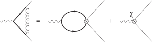
Figure 5: The matching at the scale $\mu=M$.

It is perhaps useful to think of the $\tilde{\delta}_{i}$ as the value that the coefficients of the effective lagrangian take at the matching scale, as they contain the information on modes of frequencies $\mu>M$. The $\tilde{\delta}_{i}$ will be, in general, divergent, i.e. they will have a pole in $1/\epsilon$. Let us see how to obtain these coefficients $\tilde{\delta}_{i}$ in a particular case.

As discussed in the previous section we understand that at very high energies our theory is described by a gauge theory. Therefore we have to add to the Standard Model lagrangian (already extended with technifermions) the following pieces

$$-\frac{1}{4}E_{\mu\nu}E^{\mu\nu}-\frac{1}{2}M^{2}E_{\mu}E^{\mu}+G\bar{Q}\gamma^{\mu}E_{\mu}q+{\rm h.c.}.$$ (87)

The $E_{\mu}$ vector boson (of mass $M$) acts in a large flavour group space which mixes ordinary fermions with heavy ones. (The notation in (87) is somewhat symbolic as we are not implying that the theory is vector-like, in fact we do not assume anything at all about it.)

At energies $\mu<M$ we can describe the contribution from this sector to the effective lagrangian coefficients either using the degrees of freedom present in (87) or via the corresponding four quark operator and a non-zero value for the $\tilde{\delta}_{i}$ coefficients. Demanding that both descriptions reproduce the same renormalised $ffW$ vertex fixes the value of the $\tilde{\delta}_{i}$.

Let us see this explicitly in the case where the intermediate vector boson $E_{\mu}$ is a $SU(3)_{c}\times SU(2)_{L}$ singlet. For the sake of simplicity, we take the third term in (87) to be

$$G\bar{Q}_{L}\gamma^{\mu}E_{\mu}q_{L}.$$ (88)

At energies below $M$, the relevant four quark operator is then

$$-{G^{2}\over M^{2}}(\bar{Q}_{L}\gamma^{\mu}q_{L})(\bar{q}_{L}\gamma_{\mu}Q_{L}).$$ (89)

In the limit of degenerate techniquark masses, it is quite clear that only $\tilde{\delta}_{1}$ can be different from zero. Thus, one does not need to worry about matching quark self-energies. Concerning the vertex (figure 5), we have to impose eq. (32), where now

$$\Delta\Gamma\equiv\Gamma_{E}-\Gamma_{4Q}.$$ (90)

Namely, $\Delta\Gamma$ is the difference between the vertex computed using (87) and the same quantity computed using the four quark operators as well as non zero $\tilde{\delta}_{i}$ coefficients (recall that the hat in (32) denotes renormalised quantities). A calculation analogous to that of section 4 (now the leading terms in $1/M^{2}$ are retained) leads to

$$\tilde{\delta}_{1}=-{G^{2}\over 8\pi^{2}}{m_{Q}^{2}\over M^{2}}{1\over\hat{\epsilon}}.$$ (91)

8 Integrating out heavy fermions

As we move down in energies we can integrate lower and lower frequencies with the help of the four-fermion operators (which do accurately describe physics below $M$). This modifies the value of the $\delta_{i}$

$$\delta_{i}(\mu)=\tilde{\delta}_{i}+\Delta\delta_{i}(\mu/M),\qquad\mu<M.$$ (92)

The quantity $\Delta\delta_{i}(\mu/M)$ can be computed in perturbation theory down to the scale $\Lambda_{\chi}$ where the residual interactions labelled by the index $A$ becomes strong and confine the technifermions. The leading contribution is given by a loop of technifermions.

To determine such contribution it is necessary to demand that the renormalised Green functions match when computed using explicitly the degrees of freedom $Q_{L}$, $Q_{R}$ and when their effect is described via the effective lagrangian coefficients $\delta_{i}$. The matching procedure is illustrated in figure 6.

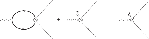
Figure 6: Matching at the scale $\mu=\Lambda_{\chi}$.

The scale $\mu$ of the matching must be such that $\mu<M$, but such that $\mu>\Lambda_{\chi}$, where perturbation theory in the technicolour coupling constant starts being questionable.

The result of the calculation in the case of degenerate masses is

$$\Delta\delta_{i}(\mu/M)=-\bar{\delta}_{i}\left(1-\hat{\epsilon}\log{\mu^{2}\over M^{2}}\right),$$ (93)

where we have kept the logarithmically enhanced contribution only and have neglected any other possible constant pieces. $\bar{\delta}_{i}$ is the singular part of $\tilde{\delta}_{i}$. The finite parts of $\tilde{\delta}_{i}$ are clearly very model dependent (cfr. for instance the previous discussion on evanescent operators) and we cannot possibly take them into account in a general analysis. Accordingly, we ignore all other terms in (93) as well as those finite pieces generated through the fierzing procedure (see discussion in previous section). Keeping the logarithmically enhanced terms therefore sets the level of accuracy of our calculation. We will call (92) the short-distance contribution to the coefficient $\delta_{i}$. General formulae for the case where the two technifermions are not degenerate in masses can be found in appendix E.

Notice that the final short distance contribution to the $\delta_{i}$ is ultraviolet finite, as it should. The divergences in $\tilde{\delta}_{i}$ are exactly matched by those in $\Delta\delta_{i}$. The pole in $\tilde{\delta}_{i}$ combined with singularity in $\Delta\delta_{i}$ provides a finite contribution.

There is another potential source of corrections to the $\delta_{i}$ stemming from the renormalization of the four fermion coupling constant $G^{2}/M^{2}$ (similar to the renormalization of the Fermi constant in the electroweak theory due to gluon exchange). This effect is however subleading here. The reason is that we are considering technigluon exchange only for four-fermion operators of the form ${\bf J}\cdot{\bf j}$, where, again, ${\bf j}$ (${\bf J}$) stands for a (heavy) fermion current (which give the leading contribution, as discussed). The fields carrying technicolour have the same handedness and thus there is no multiplicative renormalization and the effect is absent.

Of course in addition to the short distance contribution there is a long-distance contribution from the region of integration of momenta $\mu<\Lambda_{\chi}$. Perturbation theory in the technicolour coupling constant is questionable and we have to resort to other methods to determine the value of the $\delta_{i}$ at the $Z$ mass.

There are two possible ways of doing so. One is simply to mimic the constituent chiral quark model of QCD. There one loop of chiral quarks with momentum running between the scale of chiral symmetry breaking and the scale of the constituent mass of the quark, which acts as infrared cut-off, provide the bulk of the contribution[28, 29] to $f_{\pi}$, which is the equivalent of $v$. Making the necessary translations we can write for QCD-like theories

$$v^{2}\simeq n_{TC}n_{D}\frac{m_{Q}^{2}}{4\pi^{2}}\log\frac{\Lambda^{2}_{\chi}}{m_{Q}^{2}}.$$ (94)

Alternatively, we can use chiral lagrangian techniques[34] to write a low-energy bosonized version of the technifermion bilinears $\bar{Q}_{L}\Gamma Q_{L}$ and $\bar{Q}_{R}\Gamma Q_{R}$ using the chiral currents ${\bf J}_{L}$ and ${\bf J}_{R}$. The translation is

$$\bar{Q}_{L}\gamma^{\mu}Q_{L}\to\frac{v^{2}}{2}{\rm tr}U^{\dagger}{\rm i}D_{\mu}U$$ (95)

$$\bar{Q}_{L}\gamma^{\mu}\tau^{i}Q_{L}\to\frac{v^{2}}{2}{\rm tr}U^{\dagger}\tau^{i}{\rm i}D_{\mu}U$$ (96)

$$\bar{Q}_{R}\gamma^{\mu}Q_{R}\to\frac{v^{2}}{2}{\rm tr}U{\rm i}D_{\mu}U^{\dagger}$$ (97)

$$\bar{Q}_{R}\gamma^{\mu}\tau^{i}Q_{R}\to\frac{v^{2}}{2}{\rm tr}U\tau^{i}{\rm i}D_{\mu}U^{\dagger}$$ (98)

Other currents do not contribute to the effective coefficients. Both methods agree.

Finally, we collect all contributions to the coefficients $\delta_{i}$ of the effective lagrangian. For fields in the usual representations of the gauge group

$$\delta_{1} = a_{\vec{L}^{2}}\frac{G^{2}}{M^{2}}(v^{2}+n_{TC}n_{D}\frac{m_{Q}^{2}}{4\pi^{2}}\log\frac{M^{2}}{\Lambda^{2}_{\chi}})-\frac{1}{16\pi^{2}}\frac{y_{u}^{2}+y_{d}^{2}}{4}(\frac{1}{\hat{\epsilon}}-\log\frac{\Lambda^{2}}{\mu^{2}})$$ (99)

$$\delta_{2} = (a_{\vec{R}^{2}}+\frac{1}{2}a_{R_{3}^{2}})\frac{G^{2}}{M^{2}}(v^{2}+n_{TC}n_{D}\frac{m_{Q}^{2}}{4\pi^{2}}\log\frac{M^{2}}{\Lambda^{2}_{\chi}})-\frac{1}{16\pi^{2}}\frac{(y_{u}+y_{d})^{2}}{8}(\frac{1}{\hat{\epsilon}}-\log\frac{\Lambda^{2}}{\mu^{2}})$$ (100)

$$\delta_{3} = \frac{1}{2}a_{R_{3}L}\frac{G^{2}}{M^{2}}(v^{2}+n_{TC}n_{D}\frac{m_{Q}^{2}}{4\pi^{2}}\log\frac{M^{2}}{\Lambda^{2}_{\chi}})+\frac{1}{16\pi^{2}}\frac{y_{u}^{2}-y_{d}^{2}}{4}(\frac{1}{\hat{\epsilon}}-\log\frac{\Lambda^{2}}{\mu^{2}})$$ (101)

$$\delta_{4} = 0$$ (102)

$$\delta_{5} = \frac{1}{2}a_{R_{3}R}\frac{G^{2}}{M^{2}}(v^{2}+n_{TC}n_{D}\frac{m_{Q}^{2}}{4\pi^{2}}\log\frac{M^{2}}{\Lambda^{2}_{\chi}})-\frac{1}{16\pi^{2}}\frac{y_{u}^{2}-y_{d}^{2}}{4}(\frac{1}{\hat{\epsilon}}-\log\frac{\Lambda^{2}}{\mu^{2}})$$ (103)

$$\delta_{6} = \frac{1}{2}a_{R_{3}^{2}}\frac{G^{2}}{M^{2}}(v^{2}+n_{TC}n_{D}\frac{m_{Q}^{2}}{4\pi^{2}}\log\frac{M^{2}}{\Lambda^{2}_{\chi}})-\frac{1}{16\pi^{2}}\frac{(y_{u}-y_{d})^{2}}{4}(\frac{1}{\hat{\epsilon}}-\log\frac{\Lambda^{2}}{\mu^{2}}),$$ (104)

while in the case of higher representations, where only custodially preserving operators have been considered, only $\delta_{1}$ and $\delta_{2}$ get non-zero values (through $a_{{\vec{L}}^{2}}$ and $a_{{\vec{R}}^{2}}$). The long distance contribution is, obviously, universal (see section 2), while we have to modify the short distance contribution by replacing the Casimir of the fundamental representation of $SU(2)$ for the appropriate one ($1/2\to c(R)$), the number of doublets by the multiplicity of the given representation, and $n_{c}$ by the appropriate dimensionality of the $SU(3)_{c}$ representation to which the $Q$ fields belong.

These expressions require several comments. First of all, they contain the same (universal) divergences as their counterparts in the minimal Standard Model. The scale $\Lambda$ should, in principle, correspond to the matching scale $\Lambda_{\chi}$, where the low-energy non-linear effective theory takes over. However, we write an arbitrary scale just to remind us that the finite part accompanying the log is regulator dependent and cannot be determined within the effective theory. Recall that the leading ${\cal O}(n_{TC}n_{D})$ term is finite and unambiguous, and that the ambiguity lies in the formally subleading term (which, however, due to the log is numerically quite important). Furthermore only logarithmically enhanced terms are included in the above expressions. Finally one should bear in mind that the chiral quark model techniques that we have used are accurate only in the large $n_{TC}$ expansion (actually $n_{TC}n_{D}$ here). The same comments apply of course to the oblique coefficients $a_{i}$ presented in the appendix.

The quantities $a_{\vec{L}^{2}}$, $a_{\vec{R}^{2}}$, $a_{R_{3}^{2}}$, $a_{R_{3}L}$ and $a_{R_{3}R}$ are the coefficients of the four-fermion operators indicated by the sub-index (a combination of Clebsch-Gordan and fierzing factors). They depend on the specific model. As discussed in previous sections these coefficients can be of either sign. This observation is important because it shows that the contribution to the effective coefficients has no definite sign[35] indeed. It is nice that there is almost a one-to-one correspondence between the effective lagrangian coefficients (all of them measurable, at least in principle) and four-fermion coefficients.

Apart from these four-fermion coefficients, the $\delta_{i}$ depend on a number of quantities ($v$, $m_{Q}$, $\Lambda_{\chi}$, $G$ and $M$). Let us first discuss those related to the electroweak symmetry breaking, ($m_{Q}$ and $\Lambda_{\chi}$) and postpone the considerations on $M$ to the next section ($G$ will be assumed to be of ${\cal O}(1)$). $v$ is of course the Fermi scale and hence not an unknown at all ($v\simeq 250$ GeV). The value of $m_{Q}$ can be estimated from (94) since $v^{2}$ is known and $\Lambda_{\chi}$, for QCD-like technicolor theories is $\sim 4\pi v$. Solving for $m_{Q}$ one finds that if $n_{D}=4$, $m_{Q}\simeq v$, while if $n_{D}=1$, $m_{Q}\simeq 2.5v$. Notice that $m_{Q}$ and $v$ depend differently on $n_{TC}$ so it is not correct to simply assume $m_{Q}\simeq v$. In theories where the technicolor $\beta$ function is small (and it is pretty small if $n_{D}=4$ and $n_{TC}=2$) the characteristic scale of the breaking is pushed upwards, so we expect $\Lambda_{\chi}\gg 4\pi v$. This brings $m_{Q}$ somewhat downwards, but the decrease is only logarithmic. We shall therefore take $m_{Q}$ to be in the range 250 to 450 GeV. We shall allow for a mass splitting within the doublets too. The splitting within each doublet cannot be too large, as figure 4 shows. For simplicity we shall assume an equal splitting of masses for all doublets.

9 Results and discussion

Let us first summarize our results so far. The values of the effective lagrangian coefficients encode the information about the symmetry breaking sector that is (and will be in the near future) experimentally accessible. The $\delta_{i}$ are therefore the counterpart of the oblique corrections coefficients $a_{i}$ and they have to be taken together in precision analysis of the Standard Model, even if they are numerically less significant.

These effective coefficients apply to $Z$-physics at LEP, top production at the Next Linear Collider, measurements of the top decay at CDF, or indeed any other process involving the third generation (where their effect is largest), provided the energy involved is below $4\pi v$, the limit of applicability of chiral techniques. (Of course chiral effective lagrangian techniques fails well below $4\pi v$ if a resonance is present in a given channel, see also [36].)

In the Standard model the $\delta_{i}$ are useful to keep track of the $\log M_{H}$ dependence in all processes involving either neutral or charged currents. They also provide an economical description of the symmetry breaking sector, in the sense that they contain the relevant information in the low-energy regime, the only one testable at present. Beyond the Standard model the new physics contributions is parametrized by four-fermion operators. By choosing the number of doublets, $m_{Q}$, $M$, and $\Lambda_{\chi}$ suitably, we are in fact describing in a single shot a variety of theories: extended technicolor (commuting and non-commuting), walking technicolor[37] or top-assisted technicolor, provided that all remaining scalars and pseudo-Goldstone bosons are sufficiently heavy.

The accuracy of the calculation is limited by a number of approximations we have been forced to make and which have been discussed at length in previous sections. In practice we retain only terms which are logarithmically enhanced when running from $M$ to $m_{Q}$, including the long distance part, below $\Lambda_{\chi}$. The effective lagrangian coefficients $\delta_{i}$ are all finite at the scale $\Lambda_{\chi}$, the lower limit of applicability of perturbation theory. Below that scale they run following the renormalization group equations of the non-linear theory and new divergences have to be subtracted. These coefficients contain finally the contribution from scales $M>\mu>m_{Q}$, the dynamically generated mass of the technifermion (expected to be of ${\cal O}(\Lambda_{TC})$. In view of the theoretical uncertainties, to restrict oneself to logarithmically enhanced terms is a very reasonable approximation which should capture the bulk of the contribution.

Let us now proceed to a more detailed discussion of the implications of our analysis. Let us begin by discussing the value that we should take for $M$, the mass scale normalizing four-fermion operators. Fermion condensation gives a mass to ordinary fermions via chirality-flipping operators of order

$$m_{f}\simeq\frac{G^{2}}{M^{2}}\langle\bar{Q}Q\rangle,$$ (105)

through the operators listed in table 2. A chiral quark model calculation shows that

$$\langle\bar{Q}Q\rangle\simeq v^{2}m_{Q}.$$ (106)

Thus, while $\langle\bar{Q}Q\rangle$ is universal, there is an inverse relation between $M^{2}$ and $m_{f}$. In QCD-like theories this leads to the following rough estimates for the mass $M$ (the subindex refers to the fermion which has been used in the l.h.s. of (105))

$$M_{e}\sim 150{\rm TeV},\qquad M_{\mu}\sim 10{\rm TeV},\qquad M_{b}\sim 3{\rm TeV}.$$ (107)

If taken at face value, the scale for $M_{b}$ is too low, even the one for $M_{\mu}$ may already conflict with current bounds on FCNC, unless they are suppressed by some other mechanism in a natural way. Worse, the top mass cannot be reasonably reproduced by this mechanism. This well-known problem can be partly alleviated in theories where technicolor walks or invoking top-colour or a similar mechanism [38]). Then $M$ can be made larger and $m_{Q}$, as discussed, somewhat smaller. For theories which are not vector-like the above estimates become a lot less reliable.

However one should not forget that none of the four-fermion operators playing a role in the vertex effective couplings participates at all in the fermion mass determination. In principle we can then entertain the possibility that the relevant mass scale for the latter should be lower (perhaps because they get a contribution through scalar exchange, as some of them can be generated this way). Even in this case it seems just natural that $M_{b}$ (the scale normalizing chirality preserving operators for the third generation, that is) is low and not too different from $\Lambda_{\chi}$. Thus the logarithmic enhancement is pretty much absent in this case and some of the approximations made become quite questionable in this case. (Although even for the $b$ couplings there is still a relatively large contribution to the $\delta_{i}$’s coming from long distance contributions.) Put in another words, unless an additional mechanism is invoked, it is not really possible to make definite estimates for the $b$-effective couplings without getting into the details of the underlying theory. The flavour dynamics and electroweak breaking are completely entangled in this case. If one only retains the long distance part (which is what we have done in practice) we can, at best, make order-of-magnitude estimates. However, what is remarkable in a way is that this does not happen for the first and second generation vertex corrections. The effect of flavour dynamics can then be encoded in a small number of coefficients.

We shall now discuss in some detail the numerical consequences of our assumptions. We shall assume the above values for the mass scale $M$; in other words, we shall place ourselves in the most disfavourable situation. We shall only present results for QCD-like theories and $n_{D}=4$ exclusively. For other theories the appropriate results can be very easily obtained from our formulae. For the coefficients $a_{\vec{L}^{2}}$, $a_{R_{3}R}$, $a_{R_{3}L}$, etc. we shall use the range of variation [-2, 2] (since they are expected to be of ${\cal O}(1)$). Of course larger values of the scale, $M$, would simply translate into smaller values for those coefficients, so the results can be easily scaled down.

Figure 7 shows the $g_{A}^{e},g_{V}^{e}$ electron effective couplings when vertex corrections are included and allowed to vary within the stated limits. To avoid clutter, the top mass is taken to the central value 175.6 GeV. The Standard Model prediction is shown as a function of the Higgs mass. The dotted lines in figure 7 correspond to considering the oblique corrections only. Vertex corrections change these results and, depending on the values of the four-fermion operator coefficients, the prediction can take any value in the strip limited by the two solid lines (as usual we have no specific prediction in the direction along the strip due to the dependence on $\Lambda$, inherited from the non-renormalizable character of the effective theory). A generic modification of the electron couplings is of ${\cal O}(10^{-5})$, small but much larger than in the Standard Model and, depending on its sign, may help to bring a better agreement with the central value.

The modifications are more dramatic in the case of the second generation, for the muon, for instance. Now, we expect changes in the $\delta_{i}$’s and, eventually, in the effective couplings of ${\cal O}(10^{-3})$ These modifications are just at the limit of being observable. They could even modify the relation between $M_{W}$ and $G_{\mu}$ (i.e. $\Delta r$).

Figure 8 shows a similar plot for the bottom effective couplings $g_{A}^{b},g_{V}^{b}$. It is obvious that taking generic values for the four-fermion operators (of ${\cal O}(1)$) leads to enormous modifications in the effective couplings, unacceptably large in fact. The corrections become more manageable if we allow for a smaller variation of the four-fermion operator coefficients (in the range [-0.1,0.1]). This suggests that the natural order of magnitude for the mass $M_{b}$ is $\sim 10$ TeV, at least for chirality preserving operators. As we have discussed the corrections can be of either sign.

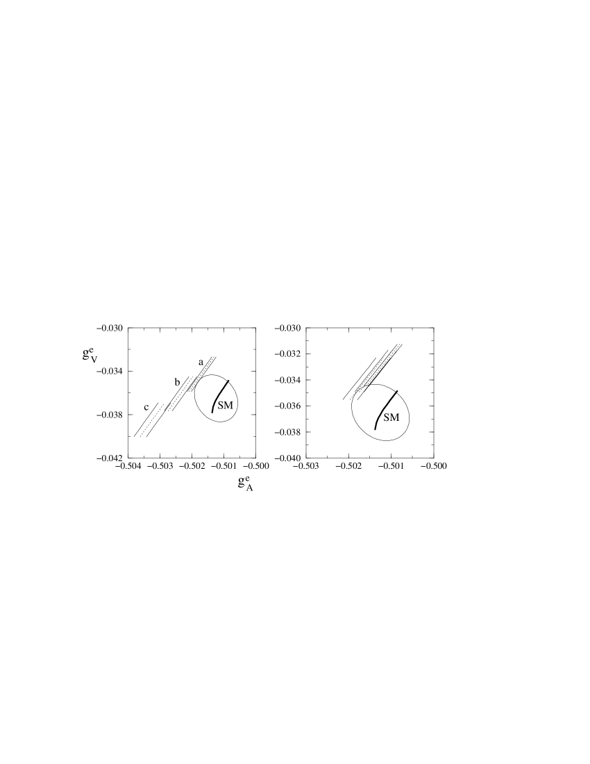
Figure 7: Oblique and vertex corrections for the electron effective couplings. The elipse indicate the 1-$\sigma$ experimental region. Three values of the effective mass $m_{2}$ are considered: 250 (a), 350 (b) and 450 GeV (c), and two splittings: 10% (right) and 20% (left). The dotted lines correspond to including the oblique corrections only. The coefficients of the four-fermion operators vary in the range [-2,2] and this spans the region between the two solid lines. The Standard Model prediction (thick solid line) is shown for $m_{t}=175.6$ GeV and $70\leq M_{H}\leq 1500$ GeV.

Figure 8: Bottom effective couplings compared to the SM prediction for $m_{t}=175.6$ as a function of the Higgs mass (in the range [70,1500] GeV). The elipses indicate 1, 2, and 3-$\sigma$ experimental regions. The dynamically generated masses are 250 (a), 350 (b) and 400 GeV (c) and we show a 20% splitting between the masses in the heavy doublet. The degenerate case does not present quantitative differencies if we consider the experimental errors. The central lines correspond to including only the oblique corrections. When we include the vertex corrections (depending on the size of the four-fermion coefficients) we predict the regions between lines indicated by the arrows. The four-fermion coefficients in this case take values in the range [-0.1,0.1].

One could, at least in the case of degenerate masses, translate the experimental constraints on the $\delta_{i}$ (recall that their experimental determination requires a combination of charged and neutral processes, since there are six of them) to the coefficients of the four-fermion operators. Doing so would provide us with a four-fermion effective theory that would exactly reproduce all the available data. It is obvious however that the result would not be very satisfactory. While the outcome would, most likely, be coefficients of ${\cal O}(1)$ for the electron couplings, they would have to be of ${\cal O}(10^{-1})$, perhaps smaller for the bottom. Worse, the same masses we have used lead to unacceptably low values for the top mass (105). Allowing for a different scale in the chirality flipping operators would permit a large top mass without affecting the effective couplings. Taking this as a tentative possibility we can pose the following problem: measure the effective couplings $\delta_{i}$ for all three generations and determine the values of the four-fermion operator coefficients and the characteristic mass scale that fits the data best. In the degenerate mass limit we have a total of 8 unknowns (5 of them coefficients, expected to be of ${\cal O}(1)$) and 18 experimental values (three sets of the $\delta_{i}$). A similar exercise could be attempted in the chirality flipping sector. If the solution to this exercise turned out to be mathematically consistent (within the experimental errors) it would be extremely interesting. A negative result would certainly rule out this approach. Notice that dynamical symmetry breaking predicts the pattern $\delta_{i}\sim m_{f}$, while in the Standard Model $\delta_{i}\sim m_{f}^{2}$.

We should end with some words of self-criticism. It may seem that the previous discussion is not too conclusive and that we have managed only to rephrase some of the long-standing problems in the symmetry breaking sector. However, the raison d’être of the present paper is not really to propose a solution to these problems, but rather to establish a theoretical framework to treat them systematically. Experience from the past shows that often the effects of new physics are magnified and thus models are ruled out on this basis, only to find out that a careful and rigorous analysis leaves some room for them. We believe that this may be the case in dynamical symmetry breaking models and we believe too that only through a detailed and careful comparison with the experimental data will progress take place.

The effective lagrangian provides the tools to look for an ‘existence proof’ (or otherwise) of a phenomenologically viable, mathematically consistent dynamical symmetry breaking model. We hope that there is any time soon sufficient experimental data to attempt to determine the four-fermion coefficients, at lest approximately.

Acknowledgements

We would like to thank M.J. Herrero, M. Martinez, J. Matias, S. Peris, J. Taron and F. Teubert for discussions. D.E. wishes to thank the hospitality of the SLAC Theory Group where this work was finished. J.M. acknowledges a fellowship from Generalitat de Catalunya, grant 1998FI-00614. This work has been partially supported by CICYT grant AEN950590-0695 and CIRIT contract GRQ93-1047.

Appendices

Appendix A  $d=4$ operators

The procedure we have followed to obtain (8–15) is very simple. We have to look for operators of the form $\bar{\psi}\Gamma\psi$, where $\psi=q_{L},\;q_{R}$ and $\Gamma$ contains a covariant derivative, $D_{\mu}$, and an arbitrary number of $U$ matrices. These operators must be gauge invariant so not any form of $\Gamma$ is possible. Moreover, we can drop total derivatives and, since $U$ is unitary, we have the following relation

$$D_{\mu}U=-U(D_{\mu}U)^{\dagger}U.$$ (108)

Apart from the obvious structure $D_{\mu}U$ which transform as $U$ does, we immediately realise that the particular form of $G_{R}$ implies the following simple transformations for the combinations $U\tau^{3}U^{\dagger}$ and $(D_{\mu}U)\tau^{3}U^{\dagger}$

$$U\tau^{3}U^{\dagger} \mapsto G_{L}\;U\tau^{3}U^{\dagger}\;G_{L}^{\dagger}$$ (109)

$$(D_{\mu}U)\tau^{3}U^{\dagger} \mapsto G_{L}\;(D_{\mu}U)\tau^{3}U^{\dagger}\;G_{L}^{\dagger}$$ (110)

Keeping all these relations in mind, we simply write down all the possibilities for $\bar{\psi}\Gamma\psi$ and find the list of operators (8–15). It is worth mentioning that there appears to be another family of four operators in which the $U$ matrices also occur within a trace: $\bar{\psi}\Gamma\psi\;{\rm tr}\;\Gamma^{\prime}$. One can check, however, that these are not independent. More precisely

$${\rm i}\bar{q}_{L}\gamma^{\mu}q_{L}\;{\rm tr}\;(D_{\mu}U)\tau^{3}U^{\dagger} = {\cal L}^{3}_{4}$$ (111)

$${\rm i}\bar{q}_{L}\gamma^{\mu}U\tau^{3}U^{\dagger}q_{L}\;{\rm tr}\;(D_{\mu}U)\tau^{3}U^{\dagger} = -{\cal L}^{1}_{4}+{\cal L}^{4}_{4}$$ (112)

$${\rm i}\bar{q}_{R}\gamma^{\mu}q_{R}\;{\rm tr}\;(D_{\mu}U)\tau^{3}U^{\dagger} = {\cal L}^{5}_{4}$$ (113)

$${\rm i}\bar{q}_{R}\gamma^{\mu}\tau^{3}q_{R}\;{\rm tr}\;(D_{\mu}U)\tau^{3}U^{\dagger} = {\cal L}^{2}_{4}+{\cal L}^{6}_{4}$$ (114)

Note that ${\cal L}^{7}_{4}$ (as well as ${\cal L}_{R}{}^{\prime}$ discussed above) can be reduced by equations of motion to operators of lower dimension which do not contribute to the physical processes we are interested in. We have checked that its contribution indeed drops from the relevant $S$-matrix elements.

Appendix B Feynman rules

We write the effective $d=4$ lagrangian as

$${\cal L}_{\rm eff}=\delta^{\prime}{\cal L}_{R}{}^{\prime}+\sum_{k=1}^{7}\delta_{k}{\cal L}^{k}_{4}$$ (115)

where $\delta_{k}$ are real coefficients that we have to determine through the matching. We need to match the effective theory described by ${\cal L}_{\rm eff}$ to both, the MSM and the underlying theory parametrized by the four-fermion operators. It has proven more convenient to work with the physical fields $W^{\pm}$, $Z$ and $\gamma$ in the former case whereas the use of the lagrangian fields $W^{1}$, $W^{2}$, $W^{3}$ and $B$ is clearly more straightforward for the latter. Thus, we give the Feynman rules in terms of both the physical and unphysical basis.

(116)

$$\phantom{{{\rm i}e\over 2s_{W}c_{w}}}\left.-\left(1-{\frac{2}{3}}s^{2}_{W}\right)\delta_{7}+{\frac{1}{3}}s^{2}_{W}\;\delta^{\prime}\right\}$$

$$+ {\frac{{\rm i}e}{2s_{W}c_{W}}}\gamma_{\mu}\gamma_{5}\left\{{\displaystyle{1\over 2}}\left(\delta_{1}+\delta_{2}-\delta_{4}+\delta_{6}\right)+\delta_{3}-\delta_{5}\right.$$

$$\phantom{{{\rm i}e\over 2s_{W}c_{W}}}\left.+\left(1-{\frac{2}{3}}s^{2}_{W}\right)\delta_{7}+{\frac{1}{3}}s^{2}_{W}\;\delta^{\prime}\right\}$$

(117)

$$\phantom{{{\rm i}e\over 2s_{W}c_{W}}}-\left.\left(1-{\frac{4}{3}}s^{2}_{W}\right)\delta_{7}+{\frac{2}{3}}s^{2}_{W}\;\delta^{\prime}\right\}$$

$$+ {\frac{{\rm i}e}{2s_{W}c_{W}}}\gamma_{\mu}\gamma_{5}\left\{{\displaystyle{1\over 2}}\left(-\delta_{1}-\delta_{2}+\delta_{4}-\delta_{6}\right)+\delta_{3}-\delta_{5}\right.$$

$$\phantom{{{\rm i}e\over 2s_{W}c_{W}}}+\left.\left(1-{\frac{4}{3}}s_{W}^{2}\right)\delta_{7}+{\frac{2}{3}}s_{W}^{2}\;\delta^{\prime}\right\}$$

(118)

(119)

(120)

$$+ {\rm i}e{\frac{1}{2\sqrt{2}s_{W}}}\gamma_{\mu}\gamma_{5}\left(\delta_{1}+\delta_{4}+\delta_{2}+\delta_{6}\right)$$

The operators ${\cal L}^{7}_{4}$ and ${\cal L}_{4}{}^{\prime}$ contribute to two-point function. The relevant Feynman rules are

(121)

(122)

Rather than giving the actual Feynman rules in the unphysical basis, we collect the various tensor structures that can result from the calculation of the relevant diagrams in table 4.

$$\begin{array}[]{l||c|c|c|c|c|c|}\mbox{Tensor structure}&\delta_{1}&\delta_{2}&\delta_{3}&\delta_{4}&\delta_{5}&\delta_{6}\\ \hline\cr{\rm i}\bar{q}_{L}\,g[\tau^{1}W\kern-7.11317pt/\kern 2.84526pt^{1}+\tau^{2}W\kern-7.11317pt/\kern 2.84526pt^{2}]q_{L}&1&&&1&&\\ {\rm i}\bar{q}_{L}\,\tau^{3}[gW\kern-7.11317pt/\kern 2.84526pt^{3}-g^{\prime}B\kern-7.11317pt/\kern 2.84526pt]q_{L}&1&&&-1&&\\ {\rm i}\bar{q}_{L}\,[gW\kern-7.11317pt/\kern 2.84526pt^{3}-g^{\prime}B\kern-7.11317pt/\kern 2.84526pt]q_{L}&&&-1&&&\\ {\rm i}\bar{q}_{R}\,g[\tau^{1}W\kern-7.11317pt/\kern 2.84526pt^{1}+\tau^{2}W\kern-7.11317pt/\kern 2.84526pt^{2}]q_{R}&&-1&&&&1\\ {\rm i}\bar{q}_{R}\,\tau^{3}[gW\kern-7.11317pt/\kern 2.84526pt^{3}-g^{\prime}B\kern-7.11317pt/\kern 2.84526pt]q_{R}&&-1&&&&-1\\ {\rm i}\bar{q}_{R}\,[gW\kern-7.11317pt/\kern 2.84526pt^{3}-g^{\prime}B\kern-7.11317pt/\kern 2.84526pt]q_{R}&&&&&-1&\end{array}$$

Table 4: Various structures appearing in the matching of the vertex and the corresponding contributions to $\delta_{1}$, …, $\delta_{6}$.

We include only those that can be matched to insertions of the operators ${\cal L}^{1}_{4},\dots,{\cal L}^{6}_{4}$ (the contributions to ${\cal L}^{7}_{4}$ and ${\cal L}_{4}{}^{\prime}$ can be determined from the matching of the two-point functions). The corresponding contributions of these structures to $\delta_{1},\dots\delta_{6}$ are also given in table 4. Once $\delta_{7}$ has been replaced by its value, obtained in the matching of the two-point functions, only the listed structures can show up in the matching of the vertex, otherwise the $SU(2)\times U(1)$ symmetry would not be preserved.

Appendix C Four-fermion operators

The complete list of four-fermion operators relevant for the present discussion is in tables 1 and 2 in section 6. It is also explained in sec. 6 the convenience of fierzing the operators in the last seven rows of table 1 in order to write them in the form ${\bf J}\cdot{\bf j}$. Here we just give the list that comes out naturally from our analysis, tables 1 and 2, without further physical interpretation. The list is given for fermions belonging to the representation ${\bf 3}$ of $SU(3)_{c}$ (techniquarks). By using Fierz transformations one can easily find out relations among some of these operators when the fermions are colour singlet (technileptons), which is telling us that some of these operators are not independent in this case. A list of independent operators for technileptons is also given in sec. 6.

Let us outline the procedure we have followed to obtain this basis in the (more involved) case of coloured fermions.

There are only two colour singlet structures one can build out of four fermions, namely

$$(\bar{\psi}\psi)(\bar{\psi}^{\prime}\psi^{\prime}) \equiv \bar{\psi}_{\alpha}\psi_{\alpha}\;\bar{\psi}^{\prime}_{\beta}\psi^{\prime}_{\beta}$$ (123)

$$(\bar{\psi}\vec{\lambda}\psi)\cdot(\bar{\psi}^{\prime}\vec{\lambda}\psi^{\prime}) \equiv \bar{\psi}_{\alpha}(\vec{\lambda})_{\alpha\beta}\psi_{\beta}\;\cdot\;\bar{\psi}^{\prime}_{\gamma}(\vec{\lambda})_{\gamma\delta}\psi^{\prime}_{\delta},$$ (124)

where, $\psi$ stands for any field belonging to the representation ${\bf 3}$ of $SU(3)_{c}$ ($\psi$ will be either $q$ or $Q$); $\alpha$, $\beta$, …, are colour indices; and the primes (^′) remind us that $\psi$ and $\bar{\psi}$ carry same additional indices (Dirac, $SU(2)$, …).

Next we clasify the Dirac structures. Since $\psi$ is either $\psi_{L}$ [it belongs to the representation $({\scriptstyle{1\over 2}},0)$ of the Lorentz group] or $\psi_{R}$ [representation $(0,{\scriptstyle{1\over 2}})$], we have five sets of fields to analyse, namely

$$\{\bar{\psi}_{L},\psi_{L},\bar{\psi}^{\prime}_{L},\psi^{\prime}_{L}\},\quad[R\leftrightarrow L];\qquad\{\bar{\psi}_{L},\psi_{L},\bar{\psi}_{R},\psi_{R}\};$$ (125)

$$\{\bar{\psi}_{L},\psi_{R},\bar{\psi}^{\prime}_{L},\psi^{\prime}_{R}\},\qquad[R\leftrightarrow L].$$ (126)

There is only an independent scalar we can build with each of the three sets in (125). Our choice is

$$\bar{\psi}_{L}\gamma^{\mu}\psi_{L}\;\bar{\psi}^{\prime}_{L}\gamma_{\mu}\psi^{\prime}_{L},\qquad[R\leftrightarrow L];$$ (127)

$$\bar{\psi}_{L}\gamma^{\mu}\psi_{L}\;\bar{\psi}_{R}\gamma_{\mu}\psi_{R}.$$ (128)

where the prime is not necessary in the second equation because $R$ and $L$ suffice to remind us that the two $\psi$ and $\bar{\psi}$ may carry different ($SU(2)$, technicolour, …) indices. There appear to be four other independent scalar operators: $\bar{\psi}_{L}\gamma^{\mu}\psi^{\prime}_{L}\;\bar{\psi}^{\prime}_{L}\gamma_{\mu}\psi_{L}$, $[R\leftrightarrow L]$; $\bar{\psi}_{L}\psi_{R}\;\bar{\psi}_{R}\psi_{L}$; and $\bar{\psi}_{L}\sigma^{\mu\nu}\psi_{R}\;\bar{\psi}_{R}\sigma_{\mu\nu}\psi_{L}$. However, Fierz symmetry implies that the first three are not independent, and the fourth one vanishes, as can be also seen using the identity $2{\rm i}\sigma^{\mu\nu}\gamma^{5}=\epsilon^{\mu\nu\rho\lambda}\sigma_{\rho\lambda}$. For each of the two operators in (126), two independent scalars can be constructed. Our choice is

$$\bar{\psi}_{L}\psi_{R}\;\bar{\psi}^{\prime}_{L}\psi^{\prime}_{R},\qquad[R\leftrightarrow L];$$ (129)

$$\bar{\psi}_{L}\psi^{\prime}_{R}\;\bar{\psi}^{\prime}_{L}\psi_{R},\qquad[R\leftrightarrow L].$$ (130)

Again, there appear to be four other scalar operators: $\bar{\psi}_{L}\sigma^{\mu\nu}\psi_{R}\;\bar{\psi}^{\prime}_{L}\sigma_{\mu\nu}\psi^{\prime}_{R}$, $[R\leftrightarrow L]$;$\bar{\psi}_{L}\sigma^{\mu\nu}\psi^{\prime}_{R}\;\bar{\psi}^{\prime}_{L}\sigma_{\mu\nu}\psi_{R}$, $[R\leftrightarrow L]$; which, nevertheless, can be shown not to be independent but related to (129) and (130) by Fierz symmetry. To summarize, the independent scalar structures are (127), (128), (129) and (130).

Next, we combine the colour and the Dirac structures. We do this for the different cases (127) to (130) separately. For operators of the form (127), we have the two obvious possibilities (Hereafter, colour and Dirac indices will be implicit)

$$(\bar{\psi}_{L}\gamma^{\mu}\psi_{L})(\bar{\psi}^{\prime}_{L}\gamma_{\mu}\psi^{\prime}_{L}),\qquad[R\leftrightarrow L];$$ (131)

$$(\bar{\psi}_{L}\gamma^{\mu}\psi^{\prime}_{L})(\bar{\psi}^{\prime}_{L}\gamma_{\mu}\psi_{L}),\qquad[R\leftrightarrow L];$$ (132)

where fields in parenthesis have their colour indices contracted as in (123) and (124). Note that the operator $(\bar{\psi}_{L}\gamma^{\mu}\vec{\lambda}\psi_{L})\cdot(\bar{\psi}^{\prime}_{L}\gamma_{\mu}\vec{\lambda}\psi^{\prime}_{L})$, or its $R$ version, is not independent (recall that $(\vec{\lambda})_{\alpha\beta}\cdot(\vec{\lambda})_{\gamma\delta}=2\delta_{\alpha\delta}\delta_{\beta\gamma}-2/3\;\delta_{\alpha\beta}\delta_{\gamma\delta}$). For operators of the form (128), we take

$$(\bar{\psi}_{L}\gamma^{\mu}\psi_{L})(\bar{\psi}_{R}\gamma_{\mu}\psi_{R})$$ (133)

$$(\bar{\psi}_{L}\gamma^{\mu}\vec{\lambda}\psi_{L})\cdot(\bar{\psi}_{R}\gamma_{\mu}\vec{\lambda}\psi_{R})$$ (134)

Finally, for operators of the form (129) and (130), our choice is

$$(\bar{\psi}_{L}\psi_{R})(\bar{\psi}^{\prime}_{L}\psi^{\prime}_{R}),\quad[R\leftrightarrow L];\quad(\bar{\psi}_{L}\vec{\lambda}\psi_{R})\cdot(\bar{\psi}^{\prime}_{L}\vec{\lambda}\psi^{\prime}_{R}),\quad[R\leftrightarrow L];$$ (135)

$$(\bar{\psi}_{L}\psi^{\prime}_{R})(\bar{\psi}^{\prime}_{L}\psi_{R}),\quad[R\leftrightarrow L];\quad(\bar{\psi}_{L}\vec{\lambda}\psi^{\prime}_{R})\cdot(\bar{\psi}^{\prime}_{L}\vec{\lambda}\psi_{R}),\quad[R\leftrightarrow L].$$ (136)

All them are independent unless further symmetries [e.g., $SU(2)_{L}\times SU(2)_{R}$] are introduced.

To introduce the $SU(2)_{L}\times SU(2)_{R}$ symmetry one just assigns $SU(2)$ indices ($i$, $j$, $k$, …) to each of the fields in (131–136). We can drop the primes hereafter since there is no other symmetry left but technicolour which for the present analysis is trivial (recall that we are only interested in four fermion operators of the form $Q\bar{Q}q\bar{q}$, thus technicolour indices must necessarily be matched in the obvious way: $Q^{A}\bar{Q}^{A}q\bar{q}$). For each of the operators in (131) and (132), there are two independent ways of constructing $SU(2)_{L}\times SU(2)_{R}$ invariants. Only two of the four resulting operators turn out to be independent (actually, the other two are exactly equal to the first ones). The independent operators are chosen to be

$$(\bar{\psi}_{L}^{i}\gamma^{\mu}\psi_{L}^{i})(\bar{\psi}^{j}_{L}\gamma_{\mu}\psi^{j}_{L})\equiv(\bar{\psi}_{L}\gamma^{\mu}\psi_{L})(\bar{\psi}_{L}\gamma_{\mu}\psi_{L}),\quad[R\leftrightarrow L];$$ (137)

$$(\bar{\psi}_{L}^{i}\gamma^{\mu}\psi_{L}^{j})(\bar{\psi}^{j}_{L}\gamma_{\mu}\psi^{i}_{L}),\quad[R\leftrightarrow L];$$ (138)

For each of the operators in (133–136), the same straightforward group analysis shows that there is only one way to construct a $SU(2)_{L}\times SU(2)_{R}$ invariant. Discarding the redundant operators and imposing hermiticity and $CP$ invariance one finally has, in addition to the operators (137) and (138), those listed below (from now on, we understand that fields in parenthesis have their Dirac, colour and also flavour indices contracted as in (137))

$$(\bar{\psi}_{L}\gamma^{\mu}\psi_{L})(\bar{\psi}_{R}\gamma_{\mu}\psi_{R}),$$ (139)

$$(\bar{\psi}_{L}\gamma^{\mu}\vec{\lambda}\psi_{L})\cdot(\bar{\psi}_{R}\gamma_{\mu}\vec{\lambda}\psi_{R}),$$ (140)

$$(\bar{\psi}_{L}^{i}\psi_{R}^{j})(\bar{\psi}_{L}^{k}\psi_{R}^{l})\epsilon_{ik}\epsilon_{jl}+(\bar{\psi}_{R}^{i}\psi_{L}^{j})(\bar{\psi}_{R}^{k}\psi_{L}^{l})\epsilon_{ik}\epsilon_{jl},$$ (141)

$$(\bar{\psi}_{L}^{i}\vec{\lambda}\psi_{R}^{j})\cdot(\bar{\psi}_{L}^{k}\vec{\lambda}\psi_{R}^{l})\epsilon_{ik}\epsilon_{jl}+(\bar{\psi}_{R}^{i}\vec{\lambda}\psi_{L}^{j})\cdot(\bar{\psi}_{R}^{k}\vec{\lambda}\psi_{L}^{l})\epsilon_{ik}\epsilon_{jl}.$$ (142)

We are now in a position to obtain very easily the custodially preserving operators of tables 1 and 2 We simply replace $\psi$ by $q$ and $Q$ (a pair of each: a field and its conjugate) in all possible independent ways.

To break the custodial symmetry we simply insert $\tau^{3}$ matrices in the $R$-sector of the custodially preserving operators we have just obtain (left columns of tables 1 and 2). However, not all the operators obtained this way are independent since one can prove the following relations

$$(\bar{q}_{R}^{i}\gamma^{\mu}Q_{R}^{j})(\bar{Q}_{R}^{j}\gamma_{\mu}[\tau^{3}q_{R}]^{i}) = (\bar{q}_{R}\gamma^{\mu}\tau^{3}Q_{R})(\bar{Q}_{R}\gamma_{\mu}q_{R})+(\bar{q}_{R}\gamma^{\mu}Q_{R})(\bar{Q}_{R}\gamma_{\mu}\tau^{3}q_{R})$$ (143)

$$\qquad-(\bar{q}_{R}^{i}\gamma^{\mu}[\tau^{3}Q_{R}]^{j})(\bar{Q}_{R}^{j}\gamma_{\mu}q_{R}^{i})$$

$$(\bar{q}_{R}^{i}\gamma^{\mu}[\tau^{3}Q_{R}]^{j})(\bar{Q}_{R}^{j}\gamma_{\mu}[\tau^{3}q_{R}]^{i}) = (\bar{q}_{R}\gamma^{\mu}Q_{R})(\bar{Q}_{R}\gamma_{\mu}q_{R})+(\bar{q}_{R}\gamma^{\mu}\tau^{3}Q_{R})(\bar{Q}_{R}\gamma_{\mu}\tau^{3}q_{R})$$ (144)

$$\qquad-(\bar{q}_{R}^{i}\gamma^{\mu}Q_{R}^{j})(\bar{Q}_{R}^{j}\gamma_{\mu}q_{R}^{i})$$

$$(\bar{q}_{R}^{i}\gamma^{\mu}[\tau^{3}q_{R}]^{j})(\bar{Q}_{R}^{j}\gamma_{\mu}[\tau^{3}Q_{R}]^{i}) = (\bar{q}_{R}\gamma^{\mu}q_{R})(\bar{Q}_{R}\gamma_{\mu}Q_{R})+(\bar{q}_{R}\gamma^{\mu}\tau^{3}q_{R})(\bar{Q}_{R}\gamma_{\mu}\tau^{3}Q_{R})$$ (145)

$$\qquad-(\bar{q}_{R}^{i}\gamma^{\mu}q_{R}^{j})(\bar{Q}_{R}^{j}\gamma_{\mu}Q_{R}^{i})$$

$$(\bar{q}_{R}^{i}\gamma^{\mu}[\tau^{3}q_{R}]^{j})(\bar{Q}_{R}^{j}\gamma_{\mu}Q_{R}^{i})\qquad\phantom{+}$$

$$+(\bar{q}_{R}^{i}\gamma^{\mu}q_{R}^{j})(\bar{Q}_{R}^{j}\gamma_{\mu}[\tau^{3}Q_{R}]^{i}) = (\bar{q}_{R}\gamma^{\mu}q_{R})(\bar{Q}_{R}\gamma^{\mu}\tau^{3}Q_{R})$$ (146)

$$\qquad+(\bar{q}_{R}\gamma^{\mu}\tau^{3}q_{R})(\bar{Q}_{R}\gamma^{\mu}Q_{R}).$$

Our final choice of custodially breaking operators is the one in the right columns of tables 1 and 2.

Appendix D Renormalization of the matter sector

Although most of the material in this section is standard, it is convenient to collect some of the important expressions, as the renormalization of the fermion fields is somewhat involved and also to set up the notation. Let us introduce three wave-function renormalization constants for the fermion fields

$$\pmatrix{u\cr d}_{L} \to Z_{L}^{1/2}\pmatrix{u\cr d}_{L},$$

$$u_{R} \to (Z_{R}^{u})^{1/2}u_{R},$$

$$d_{R} \to (Z_{R}^{d})^{1/2}d_{R}.$$ (147)

where $u$ ($d$) stands for the field of the up-type (down-type) fermion. We write

$$Z_{i}=1+\delta Z_{i}$$ (148)

We also renormalise the fermion masses according to

$$m_{f} \to m_{f}+\delta m_{f},$$ (149)

where $f=u,\;d$. These substitutions generate the counterterms needed to cancel the UV divergencies. The corresponding Feynman rules are

$$\begin{picture}(15.0,4.0)(-2.0,0.0)\put(0.0,1.5){\makebox(0.0,0.0)[c]{$q$}} \put(11.0,1.5){\makebox(0.0,0.0)[c]{$\bar{q}$}} \put(5.12,0.0){\makebox(0.0,0.0)[c]{$\times$}} \put(0.0,0.0){\line(1,0){10.0}} \put(2.5,0.0){\vector(1,0){0.1}} \put(7.5,0.0){\vector(1,0){0.1}} \end{picture}= {\rm i}\delta Z_{V}^{f}p\!\!\!/\,-{\rm i}\delta Z_{A}^{f}p\!\!\!/\,\gamma_{5}-{\rm i}\left({\frac{\delta m_{f}}{m_{f}}}+\delta Z_{V}^{f}\right)$$ (150)

$$\begin{picture}(15.0,7.0)(-2.0,0.0)\put(0.0,1.5){\makebox(0.0,0.0)[c]{$q$}} \put(11.0,1.5){\makebox(0.0,0.0)[c]{$\bar{q}$}} \put(5.25,0.0){\makebox(0.0,0.0)[c]{$\times$}} \put(0.0,0.0){\line(1,0){10.0}} \put(2.5,0.0){\vector(1,0){0.1}} \put(7.5,0.0){\vector(1,0){0.1}} \put(6.0,5.0){\makebox(0.0,0.0)[l]{$Z_{\mu}$}} \put(5.0,0.25){ \begin{picture}(1.0,1.0)(0.0,0.0)\put(0.0,0.0){\oval(0.5,0.5)[r]} \put(0.0,0.5){\oval(0.5,0.5)[l]} \end{picture}}\put(5.0,1.25){ \begin{picture}(1.0,1.0)(0.0,0.0)\put(0.0,0.0){\oval(0.5,0.5)[r]} \put(0.0,0.5){\oval(0.5,0.5)[l]} \end{picture}}\put(5.0,2.25){ \begin{picture}(1.0,1.0)(0.0,0.0)\put(0.0,0.0){\oval(0.5,0.5)[r]} \put(0.0,0.5){\oval(0.5,0.5)[l]} \end{picture}}\put(5.0,3.25){ \begin{picture}(1.0,1.0)(0.0,0.0)\put(0.0,0.0){\oval(0.5,0.5)[r]} \put(0.0,0.5){\oval(0.5,0.5)[l]} \end{picture}}\put(5.0,4.25){ \begin{picture}(1.0,1.0)(0.0,0.0)\put(0.0,0.0){\oval(0.5,0.5)[r]} \put(0.0,0.5){\oval(0.5,0.5)[l]} \end{picture}} \end{picture}= - {\rm i}e\gamma_{\mu}(v_{f}-a_{f}\,\gamma_{5})(\delta Z^{Z}_{1}-\delta Z^{Z}_{2})$$ (151)

$$- {\rm i}e\gamma_{\mu}\,Q_{f}\,(\delta Z^{Z\gamma}_{1}-\delta Z^{Z\gamma}_{2})$$

$$- {\rm i}e\gamma_{\mu}(v_{f}\,\delta Z_{V}^{f}+a_{f}\,\delta Z_{A}^{f})$$

$$+ {\rm i}e\gamma_{\mu}\gamma_{5}(v_{f}\,\delta Z_{A}^{f}+a_{f}\,\delta Z_{V}^{f})$$

$$\begin{picture}(15.0,7.0)(-2.0,0.0)\put(0.0,1.5){\makebox(0.0,0.0)[c]{$q$}} \put(11.0,1.5){\makebox(0.0,0.0)[c]{$\bar{q}$}} \put(5.25,0.0){\makebox(0.0,0.0)[c]{$\times$}} \put(0.0,0.0){\line(1,0){10.0}} \put(2.5,0.0){\vector(1,0){0.1}} \put(7.5,0.0){\vector(1,0){0.1}} \put(6.0,5.0){\makebox(0.0,0.0)[l]{$A_{\mu}$}} \put(5.0,0.25){ \begin{picture}(1.0,1.0)(0.0,0.0)\put(0.0,0.0){\oval(0.5,0.5)[r]} \put(0.0,0.5){\oval(0.5,0.5)[l]} \end{picture}}\put(5.0,1.25){ \begin{picture}(1.0,1.0)(0.0,0.0)\put(0.0,0.0){\oval(0.5,0.5)[r]} \put(0.0,0.5){\oval(0.5,0.5)[l]} \end{picture}}\put(5.0,2.25){ \begin{picture}(1.0,1.0)(0.0,0.0)\put(0.0,0.0){\oval(0.5,0.5)[r]} \put(0.0,0.5){\oval(0.5,0.5)[l]} \end{picture}}\put(5.0,3.25){ \begin{picture}(1.0,1.0)(0.0,0.0)\put(0.0,0.0){\oval(0.5,0.5)[r]} \put(0.0,0.5){\oval(0.5,0.5)[l]} \end{picture}}\put(5.0,4.25){ \begin{picture}(1.0,1.0)(0.0,0.0)\put(0.0,0.0){\oval(0.5,0.5)[r]} \put(0.0,0.5){\oval(0.5,0.5)[l]} \end{picture}} \end{picture}= - {\rm i}e\gamma_{\mu}\,Q_{f}(\delta Z^{\gamma}_{1}-\delta Z^{\gamma}_{2}+\delta Z_{V}^{f}-\delta Z_{A}^{f}\,\gamma_{5})$$ (152)

$$- {\rm i}e\gamma_{\mu}(v_{f}-a_{f}\,\gamma_{5})(\delta Z^{Z\gamma}_{1}-\delta Z^{Z\gamma}_{2})$$

$$\begin{picture}(15.0,7.0)(-2.0,0.0)\put(0.0,1.5){\makebox(0.0,0.0)[c]{$d$}} \put(11.0,1.5){\makebox(0.0,0.0)[c]{$\bar{u}$}} \put(5.25,0.0){\makebox(0.0,0.0)[c]{$\times$}} \put(0.0,0.0){\line(1,0){10.0}} \put(2.5,0.0){\vector(1,0){0.1}} \put(7.5,0.0){\vector(1,0){0.1}} \put(6.0,5.0){\makebox(0.0,0.0)[l]{$W^{+}_{\mu}$}} \put(5.0,0.25){ \begin{picture}(1.0,1.0)(0.0,0.0)\put(0.0,0.0){\oval(0.5,0.5)[r]} \put(0.0,0.5){\oval(0.5,0.5)[l]} \end{picture}}\put(5.0,1.25){ \begin{picture}(1.0,1.0)(0.0,0.0)\put(0.0,0.0){\oval(0.5,0.5)[r]} \put(0.0,0.5){\oval(0.5,0.5)[l]} \end{picture}}\put(5.0,2.25){ \begin{picture}(1.0,1.0)(0.0,0.0)\put(0.0,0.0){\oval(0.5,0.5)[r]} \put(0.0,0.5){\oval(0.5,0.5)[l]} \end{picture}}\put(5.0,3.25){ \begin{picture}(1.0,1.0)(0.0,0.0)\put(0.0,0.0){\oval(0.5,0.5)[r]} \put(0.0,0.5){\oval(0.5,0.5)[l]} \end{picture}}\put(5.0,4.25){ \begin{picture}(1.0,1.0)(0.0,0.0)\put(0.0,0.0){\oval(0.5,0.5)[r]} \put(0.0,0.5){\oval(0.5,0.5)[l]} \end{picture}} \end{picture}= - {\rm i}{\frac{e}{2\sqrt{2}s_{W}}}\gamma_{\mu}(1-\gamma_{5})\,(\delta Z^{W}_{1}-\delta Z^{W}_{2}+\delta Z_{L})$$ (153)

Here we have introduced the notation

$$\delta Z_{L}=\delta Z_{V}^{u,d}+\delta Z_{A}^{u,d},\quad\delta Z_{R}^{u,d}=\delta Z_{V}^{u,d}-\delta Z_{A}^{u,d},$$ (154)

and

$$v_{f}={\frac{I^{3}_{f}-2Q_{f}s_{W}^{2}}{2s_{W}c_{W}}},\qquad a_{f}={\frac{I^{3}_{f}}{2s_{W}c_{W}}}.$$ (155)

Note that the Feynman rules for the vertices contain additional renormalization constants which should be familiar from the oblique corrections.

The fermion self-energies can be decomposed as

$$\Sigma^{f}(p)=p\!\!\!/\,\,\Sigma_{V}^{f}(p^{2})+p\!\!\!/\,\gamma_{5}\,\Sigma_{A}^{f}(p^{2})+m\,\Sigma_{S}^{f}(p^{2})$$ (156)

By adding the conterterms one obtains de renormalised self-energies, which admit the same decomposition. One has

$$\hat{\Sigma}_{V}^{f}(p^{2}) = \Sigma_{V}^{f}(p^{2})-\delta Z_{V}^{f},$$ (157)

$$\hat{\Sigma}_{A}^{f}(p^{2}) = \Sigma_{A}^{f}(p^{2})+\delta Z_{A}^{f},$$ (158)

$$\hat{\Sigma}_{S}^{f}(p^{2}) = \Sigma_{S}^{f}(p^{2})+{\frac{\delta m_{f}}{m_{f}}}+\delta Z_{V}^{f},$$ (159)

where the hat denotes renormalised quantities. The on-shell renormalization conditions amount to

$${\frac{\delta m_{u,d}}{m_{u,d}}} = -\Sigma_{V}^{u,d}(m^{2}_{u,d})-\Sigma_{S}^{u,d}(m^{2}_{u,d})$$ (160)

$$\delta Z_{V}^{d} = \Sigma_{V}^{d}(m^{2}_{d})+2m^{2}_{d}[\Sigma^{d}_{V}{}^{\prime}(m^{2}_{d})+\Sigma^{d}_{S}{}^{\prime}(m^{2}_{d})]$$ (161)

$$\delta Z_{A}^{u,d} = -\Sigma_{A}^{u,d}(m^{2}_{u,d})$$ (162)

where $\Sigma{}^{\prime}(m^{2})=[\partial\Sigma(p^{2})/\partial p^{2}]_{p^{2}=m^{2}}$. Eq. (160) guarantees that $m_{u}$, $m_{d}$ are the physical fermion masses. The other two equations, come from requiring that the residue of the down-type fermion be unity. One cannot simultaneously impose this condition to both up- and down-type fermions. Actually, one can easily work out the residue of the up-type fermions which turns out to be $1+\delta_{\rm res}$ with

$$\delta{\rm res}=\hat{\Sigma}_{V}^{u}(m^{2}_{u})+2m^{2}_{u}\left[\hat{\Sigma}^{u}_{V}{}^{\prime}(m^{2}_{u})+\hat{\Sigma}^{u}_{S}{}^{\prime}(m^{2}_{u})\right].$$ (163)

Appendix E Effective lagrangian coefficients

In this appendix we shall provide the general expressions for the coefficients $a_{i}$ and $\delta_{i}$ in theories of the type we have been considering. The results are for the usual representations of $SU(2)\times SU(3)_{c}$. Extension to other representations is possible using the prescriptions listed in section 8.

$$a_{0} = \frac{n_{TC}n_{D}}{64\pi^{2}M_{Z}^{2}s_{W}^{2}}\left(\frac{m_{2}^{2}+m_{1}^{2}}{2}+\frac{m_{1}^{2}m_{2}^{2}\ln\frac{m_{1}^{2}}{m_{2}^{2}}}{m_{2}^{2}-m_{1}^{2}}\right)+\frac{1}{16\pi^{2}}\frac{3}{8}(\frac{1}{\hat{\epsilon}}-\log\frac{\Lambda^{2}}{\mu^{2}}),$$ (164)

$$a_{1} = -\frac{n_{TC}n_{D}}{96\pi^{2}}+\frac{n_{TC}\left(n_{Q}-3n_{L}\right)}{3\times 96\pi^{2}}\ln\frac{m_{1}^{2}}{m_{2}^{2}}+\frac{1}{16\pi^{2}}\frac{1}{12}(\frac{1}{\hat{\epsilon}}-\log\frac{\Lambda^{2}}{\mu^{2}}),$$ (165)

$$a_{8} = -\frac{n_{TC}\left(n_{c}+1\right)}{96\pi^{2}}\frac{1}{\left(m_{2}^{2}-m_{1}^{2}\right)^{2}}\left\{\frac{5}{3}m_{1}^{4}-\frac{22}{3}m_{2}^{2}m_{1}^{2}+\frac{5}{3}m_{2}^{4}\right.$$ (167)

$$+\left.\left(m_{2}^{4}-4m_{2}^{2}m_{1}^{2}+m_{1}^{4}\right)\frac{m_{2}^{2}+m_{1}^{2}}{m_{2}^{2}-m_{1}^{2}}\ln\frac{m_{1}^{2}}{m_{2}^{2}}\right\},$$

where $n_{TC}$ the number of technicolors (taken equal to 2 in all numerical discussions), $n_{D}$ is the number of technidoublets. It is interesting to note that all effective lagrangian coefficients (except for $a_{1}$) depend on $n_{D}$ and are independent of the actual hypercharge (or charge) assignment. $n_{Q}$ and $n_{L}$ are the actual number of techniquarks and technileptons. In the one-generation model $n_{Q}=3$, $n_{L}=1$ and, consequently, $n_{D}=4$. Furthermore in this model $a_{1}$ is mass independent. For simplicity we have written $m_{1}$ for the dynamically generated mass of the $u$-type technifermion and $m_{2}$ for the one of the $d$-type, and assumed that they are the same for all doublets. This is of course quite questionable as a large splitting between the technielectron and the technineutrino seems more likely and they should not necessarily coincide with techniquark masses, but the appropriate expressions can be easily inferred from the above formulae anyway.

$$\delta_{1} = {n_{D}n_{TC}G^{2}\over 16\pi^{2}M^{2}}a_{\vec{L}^{2}}\left\{{m_{1}^{2}+m_{2}^{2}\over 2}-m_{1}^{2}\left(1+{m_{1}^{2}\over m_{1}^{2}-m_{2}^{2}}\right)\log{m_{1}^{2}\over M^{2}}\right.$$ (168)

$$-m_{2}^{2}\left.\left(1+{m_{2}^{2}\over m_{2}^{2}-m_{1}^{2}}\right)\log{m_{2}^{2}\over M^{2}}\right\}$$

$$\delta_{2} = {n_{D}n_{TC}G^{2}\over 16\pi^{2}M^{2}}\left\{\left(a_{LR_{3}}-a_{RR_{3}}\right)A_{-}+a_{R_{3}^{2}}A_{+}+a_{\vec{R}^{2}}B_{+}\right\}$$ (169)

$$\delta_{3} = {n_{D}n_{TC}G^{2}\over 16\pi^{2}M^{2}}\left\{\left(a_{L^{2}}-a_{RL}\right)A_{-}+a_{R_{3}L}A_{+}\right\}$$ (170)

$$\delta_{4} = {n_{D}n_{TC}G^{2}\over 16\pi^{2}M^{2}}\;a_{\vec{L}^{2}}\left\{{m_{1}^{2}+m_{2}^{2}\over 2}+m_{1}^{2}\left(1-{m_{1}^{2}\over m_{1}^{2}-m_{2}^{2}}\right)\log{m_{1}^{2}\over M^{2}}\right.$$ (171)

$$+m_{2}^{2}\left.\left(1-{m_{2}^{2}\over m_{2}^{2}-m_{1}^{2}}\right)\log{m_{2}^{2}\over M^{2}}\right\}$$

$$\delta_{5} = {n_{D}n_{TC}G^{2}\over 16\pi^{2}M^{2}}\left\{\left(a_{LR}-a_{R^{2}}\right)A_{-}+a_{R_{3}R}A_{+}\right\}$$ (172)

$$\delta_{6} = {n_{D}n_{TC}G^{2}\over 16\pi^{2}M^{2}}\left\{\left(a_{LR_{3}}-a_{RR_{3}}\right)A_{-}+a_{R_{3}^{2}}A_{+}+a_{\vec{R}^{2}}B_{-}\right\}$$ (173)

$$\delta_{7} = 0$$ (174)

where

$$A_{\pm} = \mp m_{1}^{2}\log{m_{1}^{2}\over M^{2}}-m_{2}^{2}\log{m_{2}^{2}\over M^{2}}$$ (175)

$$B_{\pm} = \pm 2m_{1}m_{2}-m_{1}^{2}\left(1\pm{2m_{1}m_{2}\over m_{1}^{2}-m_{2}^{2}}\right)\log{m_{1}^{2}\over M^{2}}$$ (176)

$$- m_{2}^{2}\left(1\pm{2m_{2}m_{1}\over m_{2}^{2}-m_{1}^{2}}\right)\log{m_{2}^{2}\over M^{2}}.$$

We have not bothered to write the chiral divergences counterterms in the above expressions. They are identical to those of section 8. Although we have written the full expressions obtained using chiral quark model methods, one should be well aware of the approximations made in the text.

References

- [1] K.G.Wilson and J.G.Kogut, Phys. Rep. 12 (1974) 75; N. Cabbibo et al. Nucl. Phys. B158 (1979) 295; R.Dashen and H. Neuberger, Phys. Rev. Lett. 50 (1983) 1897; M. Lüscher and P.Weisz, Nucl. Phys. B318 (1989) 705; for numerical evidence see: J.Kuti et al. Phys. Rev. Lett. 71 (1988) 678; A. Hasenfratz et al. Nucl. Phys. B317 (1989) 81; G. Bhanot et al. Nucl. Phys. B353 (1991) 551; M.Göckeler et al. Nucl. Phys. B404 (1993) 517; U.M.Heller et al. Nucl. Phys. B405 (1993) 555.
- [2] G ’t Hooft, in Recent developments in Gauge Theories, G. ’t Hooft et al., eds. Plenum, New York, 1980; E.Witten, Nucl. Phys. B188 (1981) 513; S.Dimopoulos and H.Georgi, Nucl. Phys. B193 (1981) 150; N.Sakai, Z. Phys. C11 (1981) 153; H.E.Haber and R.Hempfling, Phys. Rev. Lett. 66 (1991) 1815; Y.Okada, M.Yamaguchi and T.Yanagida, Prog. Theor. Phys. 85 (1991) 1; J.Ellis, G.Ridolfi and F.Zwirner, Phys. Lett. B257 (1991) 83; for a recent review see: H.E.Haber, Perspectives on Higgs Physics II, G.L.Kane, ed. World Scientific, Singapore, 1997.
- [3] S.Heinemeyer, W.Hollik and G.Weiglein, hep-ph/9812472.
- [4] S.Weinberg, Phys. Rev. D13 (1976) 974; Phys. Rev. D19 (1979) 1277; L.Susskind, Phys. Rev. D20 (1979) 2619
- [5] E.Eichten and K.Lane, Phys. Lett. B90 (1980) 125.
- [6] M.S. Chanowitz, hep-ph/9807452.
- [7] M.Martínez, R.Miquel, L.Rolandi and R.Tenchini, preprint CERN-EP-98-027, to appear in Rev. Mod. Phys.
- [8] K.Abe et al. (the SLD collaboration), preprint SLAC-PUB-7697.
- [9] A.Dobado, D.Espriu and M.J.Herrero, Phys. Lett. B255 (1991) 405.
- [10] T.Appelquist and C.Bernard, Phys. Rev. D22 (1980) 200; A.Longhitano, Phys. Rev. D22 (1980) 1166; A. Longhitano, Nucl. Phys. B188 (1981) 118; R.Renken and M.Peskin, Nucl. Phys. B211 (1983) 93.
- [11] D.Espriu and M.J.Herrero, Nucl. Phys. B373 (1992) 117; M.J.Herrero and E.Ruiz-Morales, Nucl. Phys. B418 (1994) 431.
- [12] D.Espriu and J.Matias, Phys. Lett. B341 (1995) 332.
- [13] M.Peskin and T.Takeuchi, Phys. Rev. Lett. 65 (1990) 964; Phys. Rev. D46 (1992) 381.
- [14] S.Dimopoulos and L.Susskind, Nucl. Phys. B155 (1979) 237; E.Eichten and K.D.Lane Phys. Lett. B90 (1980) 125; E.Farhi and L.Susskind, Phys. Rep. 74 (1981) 277
- [15] Y. Nambu, Enrico Fermi Institute Report, No. EFI 88-39 (unpublished);V. A. Miransky and M. Tanabashi and K. Yamawaki, Phys. Lett. B221 (1989) 177; Mod. Phys. Lett. A4 (1989) 1043; W. A. Bardeen, C.T. Hill and M. Lindner, Phys. Rev. D41 (1990) 1647.
- [16] C.J.Gounaris, F.M.Renard and C.Verzegnassi, Phys.Rev. D52 (1995) 451; G.J. Gounaris, D.T. Papadamou, F.M. Renard, Z. Phys. C76 (1997) 333; K.Whisnant, J.M.Yang, B.L. Young and X.Zhang, Phys.Rev. D56 (1997) 467.
- [17] T.Appelquist, M.Bowick, E.Cohler and A.Hauser, Phys. Rev. D31 (1985) 1676
- [18] M.J.Herrero and E.Ruiz-Morales, Phys. Lett. B296 (1992) 397; J.Bagger, S.Dawson and G.Valencia, Nucl. Phys. B399 (1993) 364; S.Dittmaier and C.Grosse-Knetter, Phys. Rev. D52 (1995) 7276.
- [19] S.Dittmaier and C.Grosse-Knetter, Nucl. Phys. B459 (1996) 497.
- [20] P.Ciafaloni, D.Espriu, Phys. Rev. D56 (1997) 1752.
- [21] A.Dobado, M.J.Herrero and S.Penaranda, hep-ph/9903211.
- [22] Z Physics at LEP, G.Altarelli, R.Kleiss and C.Verzegnassi, eds. Yellow report CERN 89-08.
- [23] Reports of the Working Group on Precision Calculations for the Z Resonance, D.Bardin, W.Hollik and G.Passarino, eds. Yellow report CERN 95-03.
- [24] G.Altarelli, R.Barbieri and F.Caravaglios, Int. J. Mod. Phys. A13 (1998) 1031.
- [25] B.Holdom and J.Terning, Phys. Lett. B247 (1990) 88; A.Dobado, M.J.Herrero and J.Terron, Z. Phys. C50 (1991) 205; M.Golden and L.Randall, Nucl. Phys. B361 (1991) 3; S.Dawson and G.Valencia, Nucl. Phys. B352 (1991) 27; T.Appelquist and G.Triantaphyllou, Phys. Lett B278 (1992) 345; T.Appelquist and G.H.Wu, Phys. Rev. D48 (1993) 3235.
- [26] J.Gasser and H.Leutwyler, Nucl. Phys. B250 (1985) 465.
- [27] A.A.Andrianov, Phys. Lett. B157 (1985) 425; A.A.Andrianov et al., Lett. Math. Phys. 11 (1986) 217.
- [28] D.Espriu, E. de Rafael and J.Taron, Nucl. Phys. B345 (1990) 22.
- [29] A.A.Andrianov, D.Espriu and R.Tarrach, hep-ph/9803232, to appear in Nucl. Phys. B.
- [30] B.Holdom, Phys. Rev. Lett. 60 (1988) 1233.
- [31] E.Farhi and L.Susskind, Phys. Rep. 74 (1981) 277.
- [32] S. Herrlich and U. Nierste, Nucl. Phys. B455 (1995) 39, and references therein.
- [33] R.S. Chivukula, hep-ph/9803219.
- [34] H.Georgi, Weak Interactions and Modern Particle Theory, Benjamin/Cummings, Menlo Park, 1984.
- [35] R.S.Chivukula, E.H.Simmons and J.Terning, Phys. Lett. B331 (1994) 383; R.S.Chivukula, E.H.Simmons and J.Terning, Phys. Rev. D53 (1996) 5258; U.Mahanta, Phys. Rev. D55 (1997) 5848.
- [36] M.Dugan and M.Golden, Phys. Rev. D48 (1993) 4375.
- [37] B.Holdom, Phys. Rev. D24 (1981) 1441; Phys. Lett. B150 (1985) 301; V.A.Miransky, Nuovo Cim. A90 (1985) 149; K.Yamawaki, M.Bando and K.Matumoto, Phys. Rev. Lett. 56 (1986) 1335; T.Appelquist, D.Karabali and L.C.R. Wijewardhana, Phys. Rev. Lett. 57 (1986) 957; T.Appelquist and L.C.R. Wijewardhana, Phys. Rev. D35 (1987) 774 and Phys. Rev. D36 (1987) 568; T. Appelquist, M. Einhorn, T.Takeuchi and L.C.R.Wijewardhana, Phys. Lett. B220 (1989) 223; V. A. Miransky and K.Yamawaki, Mod. Phys. Lett. A4 (1989) 129; A.Matumoto, Prog. Theor. Phys. lett. 81 (1989) 277.
- [38] C.T.Hill, Phys. Lett. B345 (1995) 483; R.S.Chivukula, B.A.Dobrescu and J.Terning, Phys. Lett. B353 (1995) 289; K.Lane and E.Eichten, Phys. Lett. B352 (1995) 382; R.S.Chivukula, A.G.Cohen and E.H.Simmons, Phys. Lett. B380 (1996) 92.