LAPTH-636/98

hep-ph/9809220

May 1998

Physics at the Linear Collider

Fawzi Boudjema

Laboratoire de Physique Théorique LAPTH
Chemin de Bellevue, B.P. 110, F-74941 Annecy-le-Vieux, Cedex, France.

Abstract

The physics at the planned $e^{+}e^{-}$ colliders is discussed around three main topics corresponding to different manifestations of symmetry breaking: $W$ physics in the no Higgs scenario, studies of the properties of the Higgs and precision tests of SUSY. A comparison with the LHC is made for all these cases. The $\gamma\gamma$ mode of the linear collider will also be reviewed.

 Keywords: Linear Colliders, Photon-Photon Colliders, Polarization, Symmetry Breaking, Chiral Lagrangians, Supersymmetry, Higgs Bosons.

1 Introduction

1.1 The projects and the designs

There has been an intense activity during the last decade in the physics of a high energy $e^{+}e^{-}\;$linear collider. Several working groups in Europe, the USA and Japan have been set up. These groups have on the one hand addressed and tackled the feasibility and construction of such a machine, and on the other have by now convincingly made a strong point as concerns the advantages and benefits that such a collider can bring to our understanding of the fundamental issue in Physics: the mechanism of symmetry breaking (${\cal{S}}{\cal{S}}{\cal{B}}\;$) and the concomitant mass problem. In Europe, for instance, since 1991 five one-year-long Workshops have been organized, with three general meetings each[1]. The end of each of these Workshops has coincided with an international $e^{+}e^{-}\;$linear collider meeting where the studies of various groups in Japan, the US and Europe are summarized, compared and complemented[2]. Along side, the machine people who have been working on different designs have had regular international meetings.

There is general consensus for a machine which in a first stage would run around $500$GeV or at the top threshold with a luminosity of $10-80fb^{-1}$, and which should be upgraded to 1-2TeV. This means that ideally one should, from the start, have a machine with a length ( 15-30kms) so that there is enough space for the later adjunction of more accelerating devices which allow to reach the TeV regime. At the same time one has to increase the luminosity as the energy increases, to make up for the falling cross sections. Also, although the reason for building a linear rather than a circular collider $e^{+}e^{-}\;$is to avoid the prohibitive synchroton energy loss, there is nonetheless some energy loss due to beamstrahlung. This is a coherent radiation which occurs as a result of each beam feeling the intense electromagnetic field created by the opposite tightly dense bunch. If this radiation is not controlled, the huge photon flux (and accompanying $e^{+}e^{-}\;$pairs) will create a dirty background much like in a hadron collider. Energy, luminosity and beamstrahlung are the key parameters that enter in the designs of the various proposals and set constraints on their parameters(see for example the technical design reports[3, 4] and also[5]). Striving to have a luminosity, ${\cal{L}}$ increasing as $s$ (the cms energy squared), one should arrange to have beams with very small spot-sizes ${\sigma_{x,y}}$. However, this situation also leads to large beamstrahlung. One then has to find a compromise and allow for instance for flat beams ${\sigma_{x}}\gg{\sigma_{y}}$. This compromise is reflected in the formula for the luminosity:

$${\cal{L}}\propto(nNfE)\times\frac{N}{\sigma_{x}}\times\frac{1}{\sigma_{y}}\propto{\cal{P}}\times n_{\gamma}\times\frac{1}{\sigma_{y}}$$ (1.1)

$N$ is the number of particles per bunch, $n$ the number of bunches,$f$ the RF frequency. The first factor is the beam power ${\cal{P}}$, the second gives $n_{\gamma}$ the number of beamstrahlung photons that should be kept to a minimum.

Another important feature of the linear collider is the availability of polarization. $95\%$ degree of polarization for the electron beam is foreseen (note that SLD at SLAC has already achieved about $80\%$ beam polarization). Some studies have also shown that one could polarize the positrons ($60\%$ seems possible).

The main designs (refer to the corresponding homepages[6]) have been developed at DESY (Tesla which relies on a superconducting structure and the S-band SBLC), KEK (JLC with an option of running up to 1.5-2TeV), SLAC (NLC). All of these projects have had some test facilities and have also joined effort like with the international collaboration which successfully tested the final focus (FFTB: final focus tests facility). CERN has also a very ambitious project (CLIC), while with the financial crisis that has terribly hit Russian research, the Protvino project (VLEPP) will most probably never be realized. A layout of the CLIC design is shown in Fig. 1.

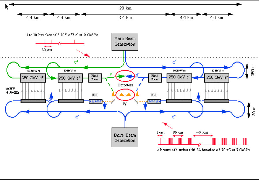
Figure 1: The 1TeV Clic Complex (from the CLIC homepage[6]).

1.2 A $\gamma\gamma\;$and $e\gamma\;$Collider

As can be seen from Fig. 1, the CLIC design allows for a second interaction region devoted to $\gamma\gamma\;$collisions. This is now an option which is taken seriously, as an add-on, in all designs. Since the organizers have asked me to spend some time on this option and since some of the Working Groups will look into the physics at these new colliders, I shall comply by going through some detail. Apart from the almost straightforward possibility to turn the $e^{+}e^{-}\;$machine into an $e^{-}e^{-}\;$mode, there is the very exciting prospect to convert either one beam of the machine or both into an intense and collimated photon beam thus turning the machine into a $e\gamma\;$or $\gamma\gamma\;$collider[7, 8]. The idea, see Fig. 2, is to focus an intense laser beam (with a frequency corresponding to a few eV) at an extremely small angle onto the single pass electron. At some conversion point (CP) a few centimeters away from the interaction point (IP) the laser photon Compton backscatters on the single-pass electron with the result that most of the energy of the electron, $E_{b}$, gets transferred to the photon beam. The latter then reaches the IP with a spread of the order of that of the original electron.

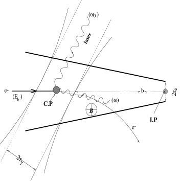
Figure 2: The laser scheme of converting an electron of the linac into a highly energetic photon (see text).

The remaining soft electron from the conversion can nonetheless be an nuisance. Not only it will scatter a few times with the photon and therefore distorts the spectrum but it can also make it to the IP. In this case the initial state would be a mixture of $e^{+}e^{-}\;$, $e\gamma\;$and $\gamma\gamma\;$thus creating again an unwanted background. One suggestion[7] is to simply sweep these remaining soft electrons by applying a strong transversal magnetic field ( 1T) within the space between the IP and the CP. But then it is still not clear what (damaging) effect this will have on the detectors especially the microvertex detector which is so crucial for Higgs studies.
A key parameter of the $\gamma\gamma\;$collider, $x_{0}$, is directly related to the maximum energy, $\omega_{max}$ that can be taken up by the photon. It is introduced through the scaled invariant mass of the original $e\gamma$ system and for a head-on hit of the laser is given by:

$$x_{0}=\frac{M_{e\gamma_{0}}^{2}}{m_{e}^{2}}-1=\frac{4E_{b}\omega_{0}}{m_{e}^{2}}\simeq(15.3)\left((\frac{E_{b}}{TeV})\right)\left(\frac{\omega_{0}}{eV}\right)\;\;\;\mbox{{\rm so that }}\;\;\omega_{\max.}=\frac{x_{0}}{x_{0}+1}E_{b}$$ (1.2)

Most of the photons are emitted at extremely small angles with the most energetic photons scattered at zero angle. With the typical angle $\theta_{0}=(m_{e}/E_{b})\sqrt{x+1}$ of order some $\mu$rd, the spread of the high-energy photon beam is thus of order some 10’s nm. The energy spread is roughly given by $\omega\approx\omega_{max}/(1+(\theta/\theta_{0})^{2})$. It is clear that the further away from the I.P. the conversion occurs, those photons that make it to the I.P. are those with the smallest scattering angle and hence with the maximum energy. These are the ones that will contribute most to the luminosity. Therefore, with a large distance of conversion one has a high monochromaticity at the expense of a small integrated (over the energy spectrum) luminosity. For those processes whose cross-section is largest for the highest possible energy, this particular set-up would be advantageous especially in reducing possible backgrounds that dominate at smaller invariant $\gamma\gamma$ masses.

From Eq. 1.2 it is clear that in order to reach the highest possible photon energies one should aim at having as large a $x_{0}$ as possible. However, one should be careful that the produced photon and the laser photon do not interact so that they create a $e^{+}e^{-}\;$pair (first threshold); the laser frequency should be chosen or tuned such that one is below the $e^{+}e^{-}\;$threshold. If we want maximum energy, it is by far best to choose the largest $x_{0}$ taking into account this restriction. The optimal $x_{0}$ is then given by $x_{0}\leq 2(1+\sqrt{2})\sim 4.83$. This value means that the photon can take up as much as $83\%$ of the beam energy. Naturally, the luminosity spectrum depends directly on the differential Compton cross-section. The original electron as well as the laser can be polarized[7], resulting in quite distinctive spectra depending on how one chooses the polarizations. The $\gamma\gamma$ luminosity spectrum is a convolution involving the differential Compton cross-sections of the two photons as well as a conversion function that depends very sensitively on the conversion distances and the characteristics of the linac beams. The energy dependence of the former function is only through the energy fraction $\sqrt{\tau}$, while the conversion function involves the $e^{+}e^{-}\;$cm energy explicitly. Realistically other considerations should be taken into account. These have to do with the laser power. In most theoretical studies it has been assumed that the density of the laser photons is such that all the electrons are converted (this assumes a conversion coefficient, $k=1$) and that multiple scattering is negligible. A compact analytical form for the conversion function is obtained in the case of a Gaussian profile for the electron beam with an azimuthal symmetry. Moreover almost all the physics analyses have been done with $b=0$. Before tackling more realistic spectra, it is worth reviewing the properties of these spectra in the simple case (with analytical formulae), in order to exhibit the importance of polarisation.

Figure 3: (a) The total luminosity spectra in the case of different combinations of the longitudinal polarizations of the linac electrons and the circular polarizations of the laser. The “classic” Weiszäcker-Williams spectrum is shown for comparison. The spectra assume a distance of conversion, $b=0$. (b) Projecting the contributions of the $J_{Z}=0$ and the $J_{Z}=2$ polarized spectrum in the peaked spectrum setting $2\lambda_{e}P_{c}=2\lambda_{e}^{\prime}P_{c}^{\prime}=-1$.

In Fig. 3a we compare the luminosity spectrum (as a function of the reduced $\gamma\gamma$ invariant mass) that one obtains by choosing different sets of polarizations for the two arms of the photon collider. First of all, in all cases and as advertised earlier one has a hard spectrum compared to the “classic” Weiszäcker-Williams spectrum. In case of no polarization at all, one obtains a broad spectrum which is almost a step function that extends nearly all the way to the maximum energy (restricted by the value of $x_{0}$). The hardest spectrum is arrived at by choosing the circular polarization of the laser ($P_{c}$) and the mean helicity of the electron ($\lambda_{e}$) to be opposite, i.e., $2\lambda_{e}P_{c}=-1$, for both arms of the collider. In the case where both arms have $2\lambda_{e}P_{c}=+1$ the spectrum has a “bell-like” shape which favours the middle range values of $\sqrt{\tau}$. In the case where the two arms of the collider have an opposite value for the product $2\lambda_{e}P_{c}$, the spectrum is almost identical to the one obtained in case of no polarization.

Figure 4: (a) Projecting the contributions of the $J_{Z}=0$ and the $J_{Z}=2$ polarized spectrum in the “broad” setting $2\lambda_{e}P_{c}=2\lambda_{e}^{\prime}P_{c}^{\prime}=1$ (with a conversion distance $b=0$). Thick lines are with a $100\%$ longitudinal polarization for the electron while the light lines are for $50\%$ longitudinal polarization. The lasers are taken to be fully right-handed. (b) As in (a) but for unpolarized electrons and where we have imposed a rapidity cut of $\eta<1$.

For the Higgs search, that is when we would like to keep an almost constant value for the differential luminosity, the “broad” spectrum that favours the $J_{Z}=0$ is highly recommended. What is very gratifying is that with $P_{c}=P_{c}^{\prime}=2\lambda_{e}=2\lambda_{e}^{\prime}=1$ the whole spectrum is accounted for almost totally by the $J_{Z}=0$ spectrum(see Fig. 4a); the $J_{Z}=2$ contributes slightly only at the higher end. This near purity of the $J_{Z}=0$ is not much degraded if the maximum mean helicity of the electron is not achieved. We show on the same figure (Fig. 4a) what happens when we change both $2\lambda_{e}$ and $2\lambda_{e}^{\prime}$ from $1$ to $.5$, keeping $P_{c}=P_{c}^{\prime}=1$. There is still a clear dominance of the $J_{Z}=0$ especially for the lower values of the centre-of-mass energy. We would like to draw attention to the fact that this effect, (increasing the $\frac{J_{Z}=0}{J_{Z}=2}$ ratio), can be further enhanced (when the maximal electron polarization is not available) by imposing rapidity cuts.

Let us now be a bit more realistic and turn to effect of the distance of conversion, keeping a blind eye on the soft electrons, and the magnetic field.

Figure 5: (a) The total luminosity spectrum with $2\lambda_{e}P_{c}=2\lambda_{e}^{\prime}P_{c}^{\prime}=-1$ (“peaked spectrum”) for different values of the conversion distance taking a spotsize $\sigma_{e}=200$ nm. (b) As in a but with $2\lambda_{e}P_{c}=2\lambda^{\prime}_{e}P_{c}^{\prime}=1$ (“broad spectrum”).

As explained above, increasing the distance of conversion filters the high energy modes and therefore the spectrum becomes more monochromatic for large values of $\gamma\gamma$ centre-of-mass energy. For the peaked spectrum, arrived at by having $2\lambda_{e}P_{c}=2\lambda^{\prime}_{e}P_{c}^{\prime}=-1$, the peaking is dramatically enhanced for a large conversion distance $b=10$cm ($\rho_{0}\simeq 0.72$). This means for example that with a conversion distance of $5$cm or $10$cm, there is almost no luminosity below $\sqrt{\tau}<0.65$. This also means (see Fig. 5a) that the spectrum is a purely $J_{Z}=0$ peaked spectrum. This is the most ideal situation to study a $J_{Z}=0$ resonance if its mass falls in this energy range, i.e, $0.7<\sqrt{\tau_{res.}}<0.82$. The $J_{Z}=2$ component that was present for the zero-distance of conversion is effectively eliminated for large distances $b>5$cm. Note that in this case if one could “manage” with a conversion distance of $0.5$cm then we almost recover the $b=0$ spectrum.
The situation is not as bright for the broad spectrum case when the interest is on small $\sqrt{\tau}$, like the search of an intermediate-mass Higgs (IMH) at a $500$ GeV $e^{+}e^{-}\;$. The nice features that were unraveled in the last paragraph (an almost pure $J_{Z}=0$ for small to moderate $\sqrt{\tau}$) are lost because the luminosity in the energy range of the IMH peak formation is totally negligible for conversion distances of order $\sim 5$cm or higher (see Fig. 5b). If one could manage with a conversion distance below $2$cm then we may hope to keep the nice features of the “broad” $J_{Z}=0$ scheme.

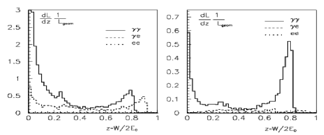
Figure 6: Luminosity spectra with $2\lambda_{e}P_{c}=2\lambda_{e}^{\prime}P_{c}^{\prime}=-1$ based on a simulation using the TESLA parameters[8]. The second spectrum correspond to having a sweeping magnet. The example we show here is in fact based on one of the most optimistic scenarios for the $\gamma\gamma\;$based on TESLA, the beams are assumed almost flat here!

This said, new simulations[8] have been conducted that have taken into account the TESLA parameters for the electron beam and studied the spectra one obtains with the option of deflecting the electron. It turns out that multiple rescattering has the effect of considerably enhancing the lower end of the spectrum. In order not to end up with too small a $\gamma\gamma\;$luminosity for large $\sqrt{\tau}$ it is advisable to deflect the electrons. Still as can be seen from Fig. 6 which adopts some optimised parameters for the TESLA design, although the deflection scheme reduces the $e\gamma\;$noise, the peak luminosity for the energetic end of the spectrum is about 5 times lower than what we obtained with the idealistic distributions. Therefore most of the studies (for reviews see[9, 10, 8]) that have been performed for this type of collider should be critically re-analyzed.

1.3 Typical cross section: the would-be-backgrounds

Figure 7: Typical sizes of cross sections for weak boson production at the linear colliders in the different modes of the machine. No convolution with luminosity spectra have been applied.

Production of new particles proceeding essentially through the s-channel in $e^{+}e^{-}\;$have cross sections of few $fb$. The main backgrounds at the linear collider will be dominated by $W$ processes. Indeed as can be seen from Fig. 7 cross sections for production of $W$’s and $Z$’s either in the $e^{+}e^{-}\;$mode or the $\gamma\gamma\;$(or for that matter the $e\gamma\;$mode) can reach a few picobarn ( we can see that the point cross section, $\sigma_{\rm point}$) is buried in the electroweak background). Fortunately the bulk of these processes is rather in the forward region, moreover they are quite sensitive to the beam polarization.

Especially in the $\gamma\gamma\;$mode, hadronic processes constitute a formidable background.

Figure 8: Direct and resolved photon contributions to bottom and charm production at $\gamma\gamma\;$collider obtained from $e^{+}e^{-}\;$at 300GeV (figure on the left) and 500GeV (on the right). The signal from a 120GeV SM Higgs as well as the additional induced $Z$ background is shown. For the resonance a smearing of 5GeV is applied. The photon spectrum is the idealised with $\lambda_{e}=.9$ $P_{c}=1$.

     

If one has a wide spectrum with invariant photon masses that extends beyond 300GeV, the bulk of these hadronic events are induced through resolved photon contributions (splitting into quarks and gluons,..). What is even more dramatic is that the initial photon polarisation will not be transferred to these constituents, thereby we loose the control of reducing backgrounds. This is especially serious for searches of the intermediate mass Higgs, IMH ( which decays into a $b\bar{b}$ pair) as a resonance[11]. The latter can be produced by selecting $J_{Z}=0$ set-up which has the advantage of drastically reducing the direct contribution $\gamma\gamma\;\rightarrow q\bar{q}$. Figure 8[12] shows how the Higgs resonance gets buried under the background, if one chooses a the laser set-up so that one has a broad spectrum. These cross sections ought to be kept in mind when we seek New Physics. Although in the previous example it has been shown how to salvage the situation, it is worth observing that for higher Higgs masses the background (into $t\bar{t}$) reduces quite a bit. Also if one wants to make precision studies of the IMH[13], then it is best to tune the machine so that the spectrum does peaks around the Higgs mass, this would though preclude a host of other studies.

2 The main issue: the mass problem and symmetry breaking

Considering that the LHC is a certainty, the fact that it has an energy reach greater than the linear collider and that the latter will certainly not be built before the LHC it is important to ask why one needs a linear collider. $e^{+}e^{-}\;$machines have always had the advantage of more than making it up for their lack of phase space by offering a clean environment which is conducive to precision measurements. For instance, we all know how difficult it is to discover the IMH at the LHC[14]. This is even more frustrating since despite the fact that SUSY does predict an IMH even if all other particles can be too heavy one will most probably have to await the high luminosity option of the LHC and combine the data of ATLAS and CMS in order to unravel it. In contrast, a 500GeV centre-of-mass energy $e^{+}e^{-}\;$collider, with a very humble luminosity $10fb^{-1}$, will discover the same Higgs in a matter of weeks (even days). This has far-reaching consequences: if no Higgs is seen even in the first phase of the LC the SUSY scenario will be out! As we will argue, even if one discovers new particles at the LHC, the main issue will be to better understand its origin. For instance even if SUSY is discovered at the LHC one would like to understand the mechanism of its breaking and reconstruct the vast array of the parameter space that plague the current phenomenological description of SUSY . As a matter of fact, probably the main raison d’être of the LC will be the understanding of symmetry breaking, a mechanism one has had till now little insight.
It should be remembered that the stunning success of the standard model, ${\cal{S}}{\cal{M}}\;$, is based on the fact that the model reconciles the gauge symmetry principle (in its non-Abelian form) with the apparent breaking of this symmetry by giving masses to the gauge bosons and fermions. The gauge symmetry principle has now been tested at the per-mil level through the universality of various gauge couplings. Even the (most evident) non-Abelian vertices ($WW\gamma,WWZ,WWWW,...$) are now badly required by precision data through their effects at the quantum level. However, to be fair these tests concern essentially the transverse polarizations of the vector bosons. Apart from the presence of the mass terms, one knows very little about the longitudinal vector components of the bosons (this is in a sense the physics of the Goldstones) and how exactly the left-handed and right-handed components of fermions interact with each other (this concerns essentially the top). These aspects are intimately related, in the ${\cal{S}}{\cal{M}}\;$description, to the Higgs mechanism. Not only the particle it predicts is still missing, though the latest global fits tend to indicate a not too heavy Higgs, but this particle does pose some very uncomfortable naturality problems which cast doubt on the whole thing and strongly suggest some alternative scenario that the planned colliders seek to uncover. In a nutshell, it is best to think of the naturality argument as being intimately related to the fact that there is no symmetry associated to the mass of an elementary spin-less particle. Chiral symmetry prevents fermions masses while gauge symmetry prevents vector boson masses with the consequence that radiative corrections to these masses are only logarithmically divergent (prior to renormalisation of course). Lack of a symmetry means that there is no reason why the mass of a scalar should be kept small and hence the infamous quadratic divergence. To remedy this, one option is to make do without an elementary scalar. One then inevitably has to deal with a strongly interacting phase of the weak interactions with the formation of condensates and bound-states and thus little calculabilty and much reduced predictivity. Or one tries to implement a symmetry. The most popular and attractive option is supersymmetry where a scalar and a fermion become the avatar of the same multiplet, and thus the scalar inherit the chiral symmetry and is protected. But then again, one knows that this symmetry is far from being perfect: the associated scalar and fermion ought to have the same mass. Then even if hints of SUSY are revealed or super-particles discovered the pressing question is how is supersymmetry broken. Lacking a fundamental theory for this breaking one has to parameterize it by a large number of parameters. Again this can be addressed through precision tests which are best conducted in $e^{+}e^{-}\;$because of its cleanliness and also because of the availability of polarisation. The latter is a wonderful tool to study symmetry breaking, ${\cal{S}}{\cal{B}}\;$. ${\cal{S}}{\cal{B}}\;$can be seen as due to the mixing and interaction of states with different quantum numbers: left and right for fermions which have different isospin numbers with the consequence that their super-partners inherit also the same quantum numbers. For bosons the presence of the Golstones and the transverse modes means that in the SUSY version one has to deal with the mixing of gauginos and Higgsinos. Thus controlling the polarisation of a ${\cal{S}}{\cal{M}}\;$state can help reach its SUSY partner which is some component of a physical SUSY state.

The remaining plan of the talk evolves around three main manifestations of the Higgs potential that describe the three main possibilities describing electroweak ${\cal{S}}{\cal{B}}\;$. 1) In the no Higgs scenario (condensates, etc..) the scalar potential does not appear, or at least is not described in terms of fundamental fields. We will then see how the physics of the Goldstones may shed light on the New Physics. 2)In the standard model description, the puzzle in the Higgs potential is the negative mass squared (associated though to the Higgs doublet) and the fact that self-interaction of the Higgs $\lambda$ (which determines the mass of the Higgs) is not fixed

$$V=\lambda\biggl{(}\Phi^{\dagger}\Phi-\frac{|\mu|^{2}}{2\lambda}\biggr{)}^{2}\;+\;V_{0}=-|\mu|^{2}\Phi^{\dagger}\Phi+\lambda|\Phi^{\dagger}\Phi|^{2}+...$$ (2.3)

If this is all we have, understanding of the properties of the Higgs will be the bread and butter of the LC. 3) In SUSY , the situation is better. $\lambda$ acquires the status of a gauge coupling, with the dramatic effect that the mass of the lightest Higgs is bounded, at tree-level, to be less than $M_{Z}$. However the negative square mass that drives symmetry breaking is still ad-hoc. There are tantalizing scenarios which embed SUSY in a grand scheme whereby the origin of the ”negative square mass” is dynamical. One such scenario is the popular minimal SUGRA model where all scalar masses are universal (with a ”positive square mass”) at the GUT scale. The heavy top drives one of the ”Higgs masses” negative as one runs down to lower energies. Supersymmetry breaking though is still obscure and, in fact, the issue is relegated to a hidden sector, although such schemes do provide sum rules like the equalities of scalar masses, and gauginos masses at the high scale. It is these kinds of sum rules and implementations that one hopes precision measurements at the LC can unravel thus giving us indirect probes of physics much beyond the TeV scale.

3 No Higgs scenarios and the $W$ couplings

Current global fits to the electroweak data tend to prefer a light Higgs mass with $M_{H}<420GEV\;95\%CL$. However in face of the discrepancy between the SLD and LEP data on the effective weak mixing angle, it has been suggested to be careful when quoting these kinds of limits. Taking the LEP data alone weakens the bound to $M_{H}<700-800GEV\;95\%CL$[15]. So especially when planning for the future when should still entertain a scenario where a Higgs is too heavy or simply not there. This said one has to implement the gauge symmetry without the scalar potential. As stressed above gauge symmetry is now sacrosanct. Already in 1994, fitting the electroweak data without the non-Abelian gauge vertices gave more than $7\sigma$ departure[16]. To implement gauge invariance an yet make do without the Higgs one retorts to a non-linear realization of symmetry breaking. To have more predictivity in this approach one can appeal to another well confirmed symmetry: the global SU(2) custodial symmetry which is the most natural explanation for the fact that once the top-bottom splitting has been taken into account the $\rho$ parameter is essentially unity. One therefore may assemble the triplet of Goldstone Bosons $\omega_{i}$ into the matrix-field $\Sigma=exp(\frac{i\omega_{\alpha}\tau^{\alpha}}{v})\;\;\;(v=246GeV)$ and define the covariant derivative (through which gauge invariance will be maintained) ${{\cal D}}_{\mu}=\partial_{\mu}\Sigma+\frac{i}{2}\left(g\frac{\tau^{i}}{2}W_{\mu}^{i}\Sigma-g^{\prime}B_{\mu}\Sigma\tau_{3}\right)$. The weak bosons mass term writes

$${{\cal L}}_{M}=\frac{v^{2}}{4}{\rm Tr}({{\cal D}}^{\mu}\Sigma^{\dagger}{{\cal D}}_{\mu}\Sigma)\;\;\;;\;\;\Sigma=exp(\frac{i\omega_{\alpha}\tau^{\alpha}}{v})\rightarrow M_{W}^{2}W^{+}_{\mu}W^{-\mu}+\frac{1}{2}M_{Z}^{2}Z_{\mu}Z^{\mu}$$ (3.4)

In this so-called non-linear realization of ${\cal{S}}{\cal{B}}\;$the mass term for the $W$ and $Z$ is formally recovered by going to the physical “frame” (gauge) where all Goldstones disappear, i.e., $\Sigma\rightarrow$1. With this description the model is not renormalizable, however it can be made finite by the introduction of a cut-off which exhibits the same dependence as that of the Higgs mass in loop effects. This cut-off represents the on-set of New Physics. We expect that before this scale is reached, which is the case with the first stage LC, the effect of the New Physics will contribute to a few operators that are not described by the minimal ${\cal{S}}{\cal{M}}\;$. In fact the above mass operator Eq.3.4 should be considered as the leading (lowest) operator in an energy expansion. With the custodial symmetry and the requirements of gauge invariance there are few other operators related to the Goldstone sector that we may write. They give contributions to the self-couplings of the weak vector bosons, especially their longitudinal parts. They can be probed both at the LHC and LC in a variety of weak boson production and scattering. For the 500GeV LC the most important operators are given by ${{\cal L}}_{9L,R}$ (for details, see[17])

$${{\cal L}}_{9R} = -ig^{\prime}\frac{L_{9R}}{16\pi^{2}}{\rm Tr}({\mbox{\boldmath$B$}}^{\mu\nu}{{\cal D}}_{\mu}\Sigma^{\dagger}{{\cal D}}_{\nu}\Sigma)$$

$${{\cal L}}_{9L} = -ig\frac{L_{9L}}{16\pi^{2}}{\rm Tr}({\mbox{\boldmath$W$}}^{\mu\nu}{{\cal D}}_{\mu}\Sigma{{\cal D}}_{\nu}\Sigma^{\dagger})$$ (3.5)

If probed efficiently these operators can tell us something about the dynamics of the Goldstones. Noting that the Godlstones are contained in the covariant derivative, ${{\cal D}}_{\mu}$, whereas the transverse are essentially described by the field-strengths and that the ${\cal{S}}{\cal{M}}\;$processes are dominated by the transverse modes, one should select the longitudinals. Thus for the above operators, one should maximise their effects by having the Goldstones contributing in the final state. Thus $f\bar{f}\rightarrow W^{+}W^{-}$ seems the most appropriate. However in the $pp$ environment this has either a huge hadronic background or can not be fully reconstructed because of the two missing neutrinos. Reverting to $pp\rightarrow W\gamma,WZ$ means that the first operator will be very poorly probed at the LHC. In $e^{+}e^{-}\;$one can disentangle between the two operators most easily through initial polarisation in $e^{+}e^{-}\rightarrow W^{+}W^{-}\;$, since the former couples only to the hypercharge component and is thus enhanced if right-handed electrons are chosen. Both can also be efficiently probed in the $\gamma\gamma\;$mode. In both $\gamma\gamma\;$and $e^{+}e^{-}\;$to optimise the limits by accessing a maximum of distributions in the kinematical variables of the decays, which is somehow reconstructing the longitudinal and transerve polarisations. To that effect one sees that by writing the $WW$ final state in terms of the four-fermions, all the helicity amplitudes are accessed.

$$\mbox{}\frac{{\rm d}\sigma(\gamma(\lambda_{1})\gamma(\lambda_{2})\rightarrow W^{+}W^{-}\rightarrow f_{1}\bar{f}_{2}f_{3}\bar{f}_{4})}{{\rm d}\cos\theta\;\;{\rm d}\cos\theta_{-}^{*}\;\;{\rm d}\phi_{-}^{*}\;\;{\rm d}\cos\theta_{+}^{*}\;\;{\rm d}\phi_{+}^{*}}=Br^{f_{1}\bar{f}_{2}}_{W}Br^{f_{3}\bar{f}_{4}}_{W}\frac{\beta}{32\pi s}\left(\frac{3}{8\pi}\right)^{2}\hfill$$

$$\sum_{\lambda_{-}\lambda_{+}\lambda^{\prime}_{-}\lambda^{\prime}_{+}}{\cal M}_{\lambda_{1},\lambda_{2};\lambda_{-}\lambda_{+}}(s,\cos\theta)\;{\cal M}_{\lambda_{1},\lambda_{2};\lambda^{\prime}_{-}\lambda^{\prime}_{+}}^{*}(s,\cos\theta)\;D_{\lambda_{-}\lambda^{\prime}_{-}}(\theta_{-}^{*},\phi_{-}^{*})\;D_{\lambda_{+}\lambda^{\prime}_{+}}(\pi-\theta_{+}^{*},\phi_{+}^{*}+\pi)$$

$$\equiv\frac{{\rm d}\sigma(\gamma(\lambda_{1})\gamma(\lambda_{2})\rightarrow W^{+}W^{-})}{{\rm d}\cos\theta}\left(\frac{3}{8\pi}\right)^{2}Br^{f_{1}\bar{f}_{2}}_{W}Br^{f_{3}\bar{f}_{4}}_{W}$$

$$\sum_{\lambda_{-}\lambda_{+}\lambda^{\prime}_{-}\lambda^{\prime}_{+}}\rho_{\lambda_{-}\lambda_{+}\lambda^{\prime}_{-}\lambda^{\prime}_{+}}^{\lambda_{1},\lambda_{2}}\;D_{\lambda_{-}\lambda^{\prime}_{-}}(\theta_{-}^{*},\phi_{-}^{*})\;D_{\lambda_{+}\lambda^{\prime}_{+}}(\pi-\theta_{+}^{*},\phi_{+}^{*}+\pi)$$ (3.6)

$${\rm with} \hskip 17.07182pt\rho_{\lambda_{-}\lambda_{+}\lambda^{\prime}_{-}\lambda^{\prime}_{+}}^{\lambda_{1},\lambda_{2}}(s,\cos\theta)=\frac{{\cal M}_{\lambda_{1},\lambda_{2};\lambda_{-}\lambda_{+}}(s,\cos\theta)\;{\cal M}_{\lambda_{1},\lambda_{2};\lambda^{\prime}_{-}\lambda^{\prime}_{+}}^{*}(s,\cos\theta)}{\sum_{\lambda_{-}\lambda_{+}}|{\cal M}_{\lambda_{1},\lambda_{2};\lambda_{-}\lambda_{+}}(s,\cos\theta)|^{2}},$$

where $\theta$ is the scattering angle of the $W^{-}$ and $\rho$ is the density matrix. A maximum likelihood fitting procedure exploiting all the decay angles permits to put very tight bounds on the $L_{9}$ parameters, whereas in the $pp$ environment on relies on a much reduced set of variables and sometimes only on the counting rate.

Figure 9: Limits on ($L_{9L}-L_{9R}$) in $e^{+}e^{-}\;$including ISR and beam polarisation.

These observations are well rendered by Fig. 9 which is a compendium of studies at both $e^{+}e^{-}\;$, $\gamma\gamma\;$and the LHC[17]. One sees that already with a $500$GeV $e^{+}e^{-}\;$collider combined with a good integrated luminosity of about $80fb^{-1}$ one can reach a precision, on the parameters that probe ${\cal{S}}{\cal{B}}\;$in the genuine tri-linear $WWV$ couplings, of the same order as what we can be achieved with LEP1 on the two-point vertices. To reach higher precision and critically probe ${\cal{S}}{\cal{B}}\;$one needs to go to $TeV$ machines. In fact, at an effective $WW$ invariant masses of order the TeV, ${\cal{S}}{\cal{B}}\;$(especially in scalar-dominated models) is best probed through the genuine quartic couplings in $WW$ scattering or even perhaps in $WWZ,ZZZ$ production (that are poorly constrained at $500$GeV). LHC could also address this particular issue but one needs dedicated careful simulations to see whether any signal could be extracted in the $pp$ environment. In this regime there is also the fascinating aspect of $W$ interaction that I have not discussed and which is the appearance of strong resonances and the study of $WW$ scattering. This would reveal another alternative to the ${\cal{S}}{\cal{M}}\;$description of the scalar sector but can only be studied at a 1.5-2TeV LC or better with a 4TeV muon collider.

4 Properties of the Higgs

Unlike the situation at the LHC, the Higgs can be very easily discovered at the LC[1] almost up to the kinematical limit through $e^{+}e^{-}\;\rightarrow ZH$ and and $WW(ZZ)$ fusions $e^{+}e^{-}\;\rightarrow\nu_{e}(e^{+})\bar{\nu}_{e}(e^{-})H$. The point is whether one can learn more from this. If one looks at the Higgs interactions in the ${\cal{S}}{\cal{M}}\;$,

$${{\cal L}}_{H,M}=(D_{\mu}\Phi)^{\dagger}(D_{\mu}\Phi)+{{\cal L}}_{Yukawa}-V$$ (4.7)

the generalized kinetic term contains the mass terms of the $W/Z$ bosons but also the couplings of the Higgs to the weak vector bosons. The latter trigger the main Higgs production mechanisms in $e^{+}e^{-}\;$. As in the previous section one can check whether there are higher order operators that modify these couplings as well as the tri-linear $WWV$ couplings. More interesting, and paving the way to the SUSY tests, is to check whether there is only one Higgs doublet which is giving mass to the weak bosons. If this is the case then only one v.e.v. is involved and thus, for instance, the $ZZH$ coupling is completely specified by the gauge couplings and the $Z$ mass. If there were more than one doublet (and hence more than one Higgs) the $ZZH_{i}$ couplings will depend on ratios of v.e.v and would therefore be smaller than if there were only one Higgs. Therefore, by precisely measuring the cross section of Higgs production one could in principle infer the presence of another Higgs. Exactly the same conclusion applies to the Yukawa couplings. Most important is the measurement of $H\rightarrow b\bar{b}$, which for example in SUSY depends crucially on $tg\beta$.
At the LC, it is possible to optimize the running conditions by lowering $\sqrt{s}$ if necessary. For example for $M_{H}<200GeV$ one could choose $\sqrt{s}\simeq 300GeV$ to maximize $e^{+}e^{-}\;\rightarrow ZH$. The other advantage over $pp$ colliders is that one can, again as in the previous section, use all topologies (all $Z$ decays may be used!). In these conditions with quite modest luminosities ( 20$fb^{-1}$) it is found[18] that one can measure the mass of the Higgs at the per-mil level. The $ZZH$ coupling may be measured at the 5per-cent level. Notice that such a precision does not seem to be enough to discriminate the ${\cal{S}}{\cal{M}}\;$Higgs with a minimal SUSY Higgs. Indeed if a large deviation in this coupling is found $hA$ production should have been observed, otherwise such a precision will not reveal the indirect presence of an extra Higgs. A slightly more hopeful conclusion holds for the $h\rightarrow b\bar{b}$ where if the mass of the pseudo-scalar Higgs is above $400GeV$, the $Br(h\rightarrow b\bar{b})$ can not be larger than about $7\%$. Simulations based on the the $ZH$ final state at $500GeV$ have found that for $M_{h}=120GeV$ the branching ratio can be measured at $7\%$ but only at $12\%$ for $M_{h}=140GeV$. More thorough simulations should be performed on this coupling. For the other couplings, branching fractions are measured with a much worse precision. Apart from this, we note that some nice checks on the spin and parity of the Higgs can be performed[1]. First in $e^{+}e^{-}\;$, from the angular distribution of the Higgs or the reconstructed $Z$, one could tell whether the parity of the particle is odd or even. Take $e^{+}e^{-}\;\rightarrow ZH$, with $x$ denoting the cosine of the scattering angle, one has

$$\frac{1}{\sigma}\frac{{\rm d}\sigma}{{\rm d}x} = (1+x^{2})\;+\;\frac{s}{8M_{Z}^{2}}\biggl{(}1+\frac{M_{Z}^{2}}{s}-\frac{M_{h}^{2}}{s}\biggr{)}^{2}(1-x^{2})\propto(1-x)^{2}+{{\cal O}}(M_{Z}^{2}/s)\rightarrow{\rm parity}\;{\rm even}$$

$$\frac{1}{\sigma}\frac{{\rm d}\sigma}{{\rm d}x} \propto (1+x^{2})\rightarrow{\rm parity}\;{\rm odd}$$ (4.8)

This may, nonetheless, prove to be an academic exercise since a $ZZ{\rm scalar}$ requires a parity-even scalar. The $\gamma\gamma\;$mode can help in many ways as far as the Higgs is concerned. First, by choosing the polarizations such that the colliding photons are in a $J_{Z}=0$ state(photons with the same helicity) producing a particle as a resonance gives its spin unambiguously. Moreover, to check for CP violation in case the scalar is an admixture of a CP even and a CP odd state, one should look for an asymmetry between the two $J_{Z}=0$ configurations, that is depending on whether both photons are right-handed or both are left-handed. Another trick for the parity measurement is to invoke linear polarisation. A parity even scalar, $O^{+}$ couples as $F_{\mu\nu}F^{\mu\nu}O^{+}$ and thereby the two photon polarizations are parallel whereas for a parity odd this combination is not possible[1]. One can also, through the measurement of the cross section $\gamma\gamma\rightarrow H\rightarrow b\bar{b}$, extract the $\Gamma(H\rightarrow\gamma\gamma)$ width assuming the branching ratio into b’s has been measured in the $e^{+}e^{-}\;$mode. A simulation has shown that this width can be measured at $6\%$[18]. Note that for these precision measurements to be possible in the $\gamma\gamma\;$mode on needs to choose a peaked set-up at the Higgs peak, otherwise the $b\bar{b}$ background is killing for a light Higgs mass. For the heavier neutral Higgses on the other hand, where the resolved photon contributions are much smaller, one can use the maximum energy possible in the $\gamma\gamma\;$mode in order to access the largest mass as a resonance. This gives a wider range than in the $e^{+}e^{-}\;$mode. Another proposal which needs more investigation, especially if no direct sign of New Physics has been observed, is to retrieve the LEP1/SLC data, or even better to run at the $Z$ peak with the LC luminosity and polarisation. One can then input the Higgs mass, the top mass which in passing can be measured with a precision of .2GeV (this is almost a ten-fold better than at the LHC ) as well as the measurement of $M_{W}$ which can be improved at the LC ($\Delta M_{W}=15MeV$). One thus have at hand some super precision observables to infer some high-scale physics. Other interesting tests concern the self-couplings of the Higgs. Within SUSY these couplings are essentially gauge couplings and thus these studies are not as motivated as if a non-susy scalar has been discovered. Unfortunately, one needs to go to high Higgs masses and energies to probe anything useful[19].

5 SUSY and SUSY breaking

If SUSY is at work it will be a matter of days for the LC to discover the lightest SUSY Higgs. Else SUSY will be shown not to be the solution to the hierarchy problem. We have just discussed the kind of checks that may be performed if only the lightest Higgs were discovered and to what extent and conditions one might infer from the precision measurements that it is actually a SUSY Higgs that one has discovered. On the optimistic side one might be lucky and discover more than one Higgs if not all of them. This occurs if the pseudo-scalar Higgs has a mass below $200-250GeV$ at the 500GeV LC. As concerns the other SUSY particles it is worth putting the LHC in the picture. Indeed if SUSY is at work, this would mean that even if the LHC has had great difficulty cornering a Higgs, it should have no problem producing plenty of coloured SUSY particles (gluinos and squarks). Many studies have shown that the LHC can cover a mass range for these particles up to 2TeV![20]. If these are not produced we would be very uncomfortable with SUSY , since a new naturality problem creeps in. LHC has also a good chance to see charginos and some neutralinos, as well as sleptons. The problem is that all the kinematically accessible particles will be accessed at once. The heavier ones cascading into the lighter ones which will in turn cascade into even lighter ones ….thus creating a very blurred and confusing picture. At least if one knew the SUSY spectrum and the SUSY parameters one can reconstruct the original picture. But we will not, and if one takes an unbiased attitude one will have the formidable task to measure a large number of parameters. On the other hand, once SUSY is discovered it is exactly this, measuring the SUSY parameters, that will be a priority. This is because one expects these parameters not to be completely haphazard but show some simple structure that betrays some common origin. Due to the nature of the supersymmetry transformations this may even tie this model with gravity. There is also circumstantial evidence that the unification of the gauge couplings occurs within SUSY . It is then utterly crucial to test whether the unification of other parameters occurs as well. The answer to these questions gives an information on physics at scale orders of magnitude from the present ones, unreachable by any collider. One has then to retort to ingenuity to extract this information from the upcoming colliders.

Some simulations for the extraction of parameters has been attempted for the LHC[20]. However it is important to stress that these checks were done with the assumption of an underlying model, minimal SUGRA that contains only a few parameters. Although the parameters are extracted with a good precision it must be remembered that these studies only confirm whether a specific model is at work. The situation with supersymmetry breaking may prove to be more complicated, so ideally one would like to measure the parameters with no a priori assumption about the model. This will, probably, not be possible at the LHC.

In this respect the LC is invaluable. First, it offers a complementarity with the LHC which is better at discovering the non-coloured particles which, by the way, in many models (unification models) have much smaller masses than the coloured-ones. Second and most important, not only one has a far cleaner environment but one can optimize the energy of the machine so that only very few thresholds are crossed at a time. Thus the confusing mixing of final states with the cascade decays is avoided. There will probably be no SUSY background to SUSY signals, or else one would know how to simulate the SUSY background. Third and as important is to make full use of the power of polarisation, which takes all its meaning for a theory whose inner stucture is based on spin/chirality symmetry! Take for instance the case of sfermions. Even in the simple case of sfermions, SUSY predicts that to each fermion chirality corresponds a sfermion. Since SUSY is broken each of these sfermion $\tilde{l}_{R,L}$ may acquire a different mass (beside a so-called $D$-term contribution of gauge origin but involving the unknown $tg\beta$). What is more, electroweak ${\cal{S}}{\cal{B}}\;$mixes these two states, fortunately the effect is proportional to the mass of the corresponding fermion, but involves yet two other parameters ($\mu$ and the $A_{f}$ tri-linear couplings). Even in the case of the first and second family where the latter problem is not present, one still has a few parameters to determine. One should also make sure that one is identifying the right (correct) sfermion. That is where polarisation comes in handy. By selecting or reconstructing the chirality of the usual fermions one is almost directly picking up and unambiguously identifying the appropriate sfermion because of the fact that both fermion and sfermions share some common quantum numbers. This strategy is either not available at the LHC (initial polarisation) or too difficult to implement (final state polarisation, as we saw with $W$ physics). Once the identifications have been made, one can measure masses (and possibly other parameters) and then check some mass relations without relying on any model.

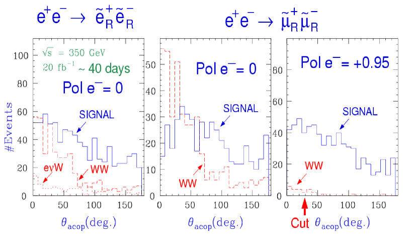
Figure 10: Effect of polarization on the muon acoplanarity angle for right-smuon and selectron production with the decay $\tilde{\mu,(e)}_{R}\rightarrow\mu,(e)\chi^{0}$. The slepton mass is 142GeV and the LSP is 118GeV, $\sqrt{s}=350GeV$ and ${{\cal L}}=20fb^{-1}$. The degree of polarisation is also shown[21].

For instance, take the pair production of a right-handed smuon which most probably will decay into the LSP neutralino and a muon. The signature is the same as that of $W$ pair production with the $W$’s decaying into muons and neutrinos and would constitute a formidable background. The use of polarisation becomes almost a must. First of all, $W$ pair production which is essentially an SU(2) weak process can be switched off by choosing right-handed electrons. Indeed, at high-energy one recovers the symmetric case where the $Z$ and $\gamma$ separate into the orthogonal $W^{0}$ and $B$ (hypercharge). The former not coupling to right-handed states. On the other hand the same argument shows that if only the hypercharge boson is exchanged and the fact that the hypercharge of the right-hand electron is twice that of the left-handed one, right smuon production will be four times larger than with left-handed $e^{-}$. Thus polarization achieves three things: tags the nature of the smuon (right-handed) independently of how it decays, increases the signal cross section and dramatically decreases the background. This is well rendered by the full simulation of the Japanese group (see Fig. 10) which has conducted some first-class studies[21] to which I will refer extensively. In the same figure the case of the selectron is also shown. The latter has more background from single $W$ production that also vanish for right-handed electrons. Once the smuon production has been optimized, one can either infer the mass from a threshold scan which is independent of the decay or as is the case here, the measurement of the end-points of the muon energy which give both the smuon mass and the LSP mass. A combined fit, for the case above and for a modest luminosity $20fb^{-1}$, gives these masses at the $1\%$ level. One more thing, to confirm the scalar nature of the smuon one can look at its angular distribution which should show a $sin^{2}\theta$ dependence. In the case of the right-handed selectron, this will not be the case since even with a right-handed electron on has to deal with a t-channel neutralino exchange. For the same reason as above only the bino component of the neutralino will be selected. If this component is not negligible one should observe a forward peak (see Fig. 11). This component is a function of the gaugino parameters $M_{1,2}$, the $\mu$ parameter and $tg\beta$. With the knowledge of $\chi^{0}_{1}$ one can measure how much of the LSP is bino.

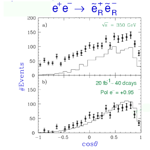
Figure 11: Same parameters as in the previous figure for the scattering angle of the right-handed selectron[21].

The mass of the right-selectron is based on the same idea as in the smuon case. One can thus already with two processes ($\tilde{\mu}^{+}_{R}\tilde{\mu}_{R}^{-},\tilde{e}^{+}_{R}\tilde{e}_{R}^{-}$) test the universality of the scalar masses (at least, at this point, for the right-sfermion masses of the first two generations) and constrain somehow the neutralino mixing matrix.

As one increases the energy new thresholds may open up, for instance the production of a selectron-right with a selectron-left. This occurs only through a t-channel neutralino. Again if one polarizes the electron to be right-handed not only one tremendously reduces the background but also one has a better handle on the signal. In this case the neutralino is projected onto the bino component that was present in $\tilde{e}^{+}_{R}\tilde{e}^{-}_{R}$. Second if both selectron species decay into an electron/positron, we know that the final electron is associated with $\tilde{e}^{-}_{R}$. The end-point energies of the final positron will reconstruct the mass of the $\tilde{e}^{+}_{L}$. Again a precision of $1\%$ is achieved. Note that left-handed electron polarisation allows in principle to access the wino component of the neutralino. With these scalar masses more general mass relations (and hence models) can be checked[22].

Similar analyses exploiting the power of polarisation can be done in the production of neutralinos and charginos. Chargino pair production goes through a t-channel sneutrino exchange as well as a s-channel $Z,\gamma$. The former can be switched off with a right-handed electron polarization which also, through the selection of the hypercharge component of neutral vector bosons, picks up only the higgsino component of the chargino, therefore this polarisation alone will give us the composition of the chargino. Again from the energy end-points of the decay products one can reconstruct the mass of the chargino with a very good precision. By combining the information from $e^{+}e^{-}_{R}\rightarrow\tilde{e}_{R}^{+}\tilde{e}_{R}^{-}$ and this reaction we can fit the parameters of the chargino-neutralino mass matrix $M_{1},M_{2},\mu,tg\beta$ and check for the GUT relation $M_{1}=\frac{5}{3}tg^{2}\theta_{W}\;M_{2}$. Fig. 12 shows the result of the fit for a simulation based on SUGRA, but of course no SUGRA hypothesis has been made in the fits. The results are impressive.

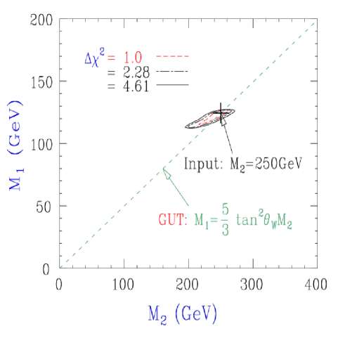
Figure 12: Results of a global fit using $e^{+}e^{-}_{R}\rightarrow\tilde{e}_{R}^{+}\tilde{e}_{R}^{-}$ and $e^{+}e^{-}_{R}\rightarrow\chi^{+}_{1}\chi^{-}_{1}$, to reconstruct $M_{1},M_{2}$ [21]

More can be done with the processes studied so far. With the left-handed electron polarisation one is sensitive to the sneutrino channel and thus would measure or constrain its mass. Needless to say that as more channels become available one can reconstruct more fundamental parameters. Polarization will be useful if not essential. For instance in the case of the third family one would like to measure the tri-linear terms $A_{f}$ beside the $U(1)$ and $SU(2)$ scalar masses as well as $\mu$ and $-tg\beta$ if these are not already measured. Both $A_{f}$ and $\mu$ are contained in the angle $\theta_{f}$ which mixes the left and right sfermions. This angle can be easily measured by measuring either the cross section for a right-handed or a left-handed electron as seen from Eq. 5 ($q_{f}$ is the charge of the sfermion)

$${{\cal M}}_{L} = {{\cal M}}_{0}\biggl{(}|q_{f}|+\frac{1}{s_{W}^{2}c_{W}^{2}}(\frac{1}{2}-s_{W}^{2})(\frac{1}{2}\cos^{2}\theta_{f}\;-\;|q_{f}|s_{W}^{2})\frac{s}{s-M_{Z}^{2}}\biggr{)}$$

$${{\cal M}}_{R} = {{\cal M}}_{0}\biggl{(}|q_{f}|-\frac{1}{c_{W}^{2}}(\frac{1}{2}\cos^{2}\theta_{f}\;-\;|q_{f}|s_{W}^{2})\frac{s}{s-M_{Z}^{2}}\biggr{)}$$ (5.9)

Decays of the third generation sfermions will also be very informative provided one can measure the polarization of the decay products, as in the case of $\tilde{\tau}$’s. These few examples make it clear that a LC will be invaluable for precision measurements of the SUSY parameters. One last word, the $\gamma\gamma\;$mode will not be as helpful as the $e^{+}e^{-}\;$mode. The reason is that in $\gamma\gamma\;$cross sections (at tree-level) are completely determined once the mass is known or measured. Reconstruction of the parameters could only be gleaned through a study of decays.

6 Conclusions

There is no doubt that the construction of a LC even if done after the LHC will allow some crucial tests as concerns our understanding of symmetry breaking and would very nicely complement the LHC program. Recently the TESLA people have shown that one can achieve even higher luminosities, $500fb^{-1}$[23]. This will allow even more powerful precision tests as the ones that we went through in this summary.

Acknowlegments: I would like to express my appreciation to the organizers for providing us a superb atmosphere and excellent food. There could not have been a better place than IUCCA for such a kind of Workshop. I would also like to thank the theory division of TIFR-Mumbai for the invitation.

References

-
[1]
Proc. of the Workshop on Collisions at GeV: The Physics
Potential, ed. P. Zerwas, DESY-92-123A,B(1992); DESY-93-123C (1993);
DESY-96-123D (1996).
Also E. Accomondo et al., Phys. Rep. (1998). -
[2]
Physics and Experiments with Linear Colliders,
1. Finland: ed. by R. Orava, P. Eerola and M. Nordberg, World Scientific (1992) 1.
2. Hawai: F.A. Harris et al.,, World Scientific, 1994.
3. Japan: ed. by A. Miyamoto and Y. Fujii, World Scientific, 1996. - [3] R. Brinkman, G. Materlik, J. Rossbaach and A. Wagner, Conceptual Design of a 500GeV Linear Collider with Integrated X-ray Laser Facility, DESY 1997-048 and ECFA 1997-182.
- [4] Physics and technology of the Next Linear Collider: A Report submitted to Snowmass ’96 By NLC ZDR Design Group and NLC Physics Working Group (S. Kuhlman et al.). hep-ex/9605011 .
- [5] H. Murayama and M.E. Peskin, Ann. Rev. of Nucl. and Part. Sci. 46 (1996) 533. hep-ex/9606003.
-
[6]
For detailed information on the designs, please refer to the homepages:
Tesla http://www-mpy.desy.de/lc-cdr/tesla/tesla.html
Desy S-band http://www-mpy.desy.de/lc-cdr/s-band/s-band.html
JLC http://www-jlc.kek.jp/index-e.html
NLC http://nlc.physics.upenn.edu/nlc/nlc.html
CLIC http://www.cern.ch/CERN/Divisions/PS/CLIC/Welcome.html. -
[7]
I.F. Ginzburg, G.L. Kotkin, V.G. Serbo and V.I. Telnov, Sov. ZhETF Pis’ma
34 (1981) 514 [JETP Lett. 34 491 (1982)];
I.F. Ginzburg, G.L. Kotkin, V.G. Serbo and V.I. Telnov, Nucl. Instrum. Methods 205 (1983) 47;
I.F. Ginzburg, G.L. Kotkin, S.L. Panfil, V.G. Serbo and V.I. Telnov, ibid 219 (1984) 5;
V.I. Telnov, ibid A294 (1990) 72;
V.I. Telnov, Proc. of the Workshop on “Physics and Experiments with Linear Colliders”, Saariselkä, Finland, eds. R. Orawa, P. Eerola and M. Nordberg, World Scientific, Singapore (1992) 739;
V.I. Telnov, in Proceedings of the IXth International Workshop on Photon-Photon Collisions., edited by D.O. Caldwell and H.P. Paar, World Scientific, (1992) 369. - [8] R. Brinkman et al., Nucl. Instrum. Methods A406 (1998) 13. hep-ex/9707017 .
- [9] M. Baillargeon, G. Bélanger and F. Boudjema, in Proceedings of Two-photon Physics from DANE to LEP200 and Beyond, Paris, eds. F. Kapusta and J. Parisi, World Scientific, 1995 p. 267; hep-ph/9405359.
- [10] S. Brodsky and P. Zerwas, Proceedings of Workshop on Gamma-Gamma Colliders Berkeley, USA, 1994, Nucl. Inst.&Meth. A355 (1995) 19.
- [11] O.J. P. Eboli, M.C. Gonzalez-Garcia, F. Halzen and D. Zeppenfeld, Phys. Rev. D48 (1993) 1430.
- [12] M. Baillargeon, G. Bélanger and F. Boudjema, Phys. Rev. D51 (1995) 4712.
-
[13]
D.L. Borden, D.A. Bauer, D.O. Caldwell, SLAC-PUB-5715, UCSB-HEP-92-01 (1992).
D.L. Borden, Proceedings of Workshop on Physics and Experiments with Linear Colliders, Eds. F.A. Harris et al. (World Scientific, 1994) 323. -
[14]
For the SM Higgs search at the LHC see: E. Richter-Was et al., ATLAS note
Phys-No-048 (1995).
for the SUSY couterpart, see ibid Phys-No-048 (1995). - [15] D. Schildknecht Invited talk at 21st International School of Theoretical Physics (USTRON 97), Ustron, Poland, 19-24 Sep 1997. Acta Phys. Pol. B28 (1997) 2291.hep-ph/9711314; G. Degrassi, P. Gambino, M. Passera, A. Sirlin, (Munich, Phys. Lett. B418 (1998) 209-213. hep-ph/9708311 P. Gambino and A. Sirlin, Phys. Rev. Lett. 73 (1994) 621.
- [16] S. Dittmaier, D. Schildknecht and G. Weiglein, BI-TP 95/31, hep-ph/9510386; S. Dittmaier, D. Schildknecht and M. Kuroda Nucl. Phys. B426 (1994);P. Gambino and A. Sirlin, Phys. Rev. Lett. 73 (1994) 621.
- [17] F. Boudjema, Invited talk at the Workshop on Physics and Experiments with Linear Colliders, Morioka, Japan, 1995, eds. A. Miyamoto et al.,, World Scientific, 1996, p. 199.
- [18] R. J. Van Kooten, Invited talk at the Workshop on Physics and Experiments with Linear Colliders, Morioka, Japan, 1995, eds. A. Miyamoto et al.,, World Scientific, 1996, p. 80. See also any of the sections on Higgs Physics in [1] and [2].
- [19] G. Gounaris, F.M. Renard and D. Schildknecht, Phys. Lett. B 83 (1979) 191 and (E) B 89 (1980) 437. V. Barger and T. Han, Mod. Phys. Lett. A5 (1990) 667. F. Boudjema and E. Chopin, Z. Phys. C73 (1996) 85. V. Ilyin et al.,, Phys. rev. D 54 (1996) 6717. In the context of the MSSM, see A. Djouadi, H. Haber and P.M. Zerwas, Phys. Lett. B375 (1996) 46. P. Osland and P. N. Pandita, hep-ph/9806351.
- [20] For a nice recent review, see F. Paige, BNL-HET-98/1, hep-ph/9801254, to appear in TASI 97, Supersymmetry, Supergarvity adn Supercolliders.
-
[21]
T. Tsukamoto, K. Fujii, H. Murayama, M. Yamaguchi and Y. Okada. Phys. Rev. D51 (1995) 3153.
M.M. Nojiri, K. Fujii and T. Tsukamoto, Phys. Rev. D54 (1996) 6756. For an extremely nice summary, see K. Fujii, in Physics and Experiments with Linear Colliders, Morioka, Japan, p. 283 Op. cit. - [22] See for instance M. Peskin, in Physics and Experiments with Linear Colliders, Morioka, Japan, p. 248 Op. cit.
- [23] For more information refer to the homepage of the 2nd ECFA-DESY Study: http://www.desy.de/conferences/ecfa-desy-lc98.html