Optimized Perturbation Theory at Finite Temperature††thanks:
Talk presented at “Thermal Field
Theories and Their Applications”,
(Regensburg, Germany, August 10-14, 1998)
— Renormalization and Nambu-Goldstone theorem in Theory —
Abstract
The optimized perturbation theory (OPT) at finite temperature () recently developed by the present authors is reviewed by using theory with spontaneous symmetry breaking. The method resums automatically higher loops (including the hard thermal loops) at high and simultaneously cures the problem of tachyonic poles at relatively low . We prove that (i) the renormalization of the ultra-violet divergences can be carried out systematically in any given order of OPT, and (ii) the Nambu-Goldstone theorem is satisfied for arbitrary and for any given order of OPT.
I Introduction
Naive perturbation theory is known to break down at finite temperature (). The two reasons are the existence of hard thermal loops (HTL) at high [2] and the emergence of tachyonic poles at relatively low [3]. If one adopts self-consistent resummation methods, HTL can be summed and tachyonic poles can be removed. However, most of the self-consistent methods proposed so far have difficulties of renormalization [4] and/or the violation of the Nambu-Goldstone theorem [5] at finite .
In this talk, we show that a new loop-wise expansion at finite recently developed by the present authors [6] can solve these problems.
Our starting point is the optimized perturbation theory (OPT) which is a generalization of the mean-field method [7] and is known to work in various quantum systems [8]. Its application to field theory at finite has been first considered by Okopińska [9] and Banerjee and Mallik [10]. We further develop the idea and prove the renormalizability and the Nambu-Goldstone (NG) theorem in theory at finite order by order in OPT.
The organization of this talk is as follows. In section II, we introduce a loop-wise expansion on the basis of OPT. The renormalization of UV divergences and the realization of the NG theorem in this method are also discussed. In section III, OPT is applied for the model which is a low energy effective theory of QCD. Summary and concluding remarks are given in Section IV.
II Optimized Perturbation at
A Hard thermal loops and tachyonic poles
Let us illustrate, by using theory, the reason why the naive perturbation theory at finite breaks down;
| (1) |
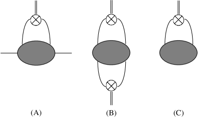
We first consider the case . The lowest order self-energy diagram Fig.1 (A) is at high . However, Fig.1 (B) is . Furthermore, higher powers of arise in higher loops; e.g. the n-loop diagram in Fig.1 (C) is . Thus, the validity of the perturbation theory breaks down when because the higher order diagrams are larger than lower ones. Therefore, one should at least resum cactus diagrams to get sensible results at high [3]. Physics behind this resummation is the well-known Debye screening mass in the hot plasma.
When and the system has spontaneous symmetry breaking (SSB), the naive perturbation shows another problem. The tree-level mass in this case is defined as
| (2) |
where is the thermal expectation value of . As increases, decreases. Then becomes negative (tachyonic) even before the critical temperature is reached. If this happens, the naive perturbation using the tree-level propagator does not make sense and certain resummation should be carried out [11]. Note that, for , there is no reason to believe that only the cactus diagrams shown in Fig.1 are dominant; there exists a three-point vertex which is not negligible for .
B Problems in self-consistent resummation methods
Self-consistent resummation method is a procedure to improve perturbation theory at finite and to avoid the problems in Sec. II A. However, the method has other difficulties [4, 5].
In the naive perturbation theory, there arises no new UV divergences at because of the natural cutoff from the Boltzmann distribution function. Therefore, all the UV divergences at finite are canceled by the counter terms prepared at [12].
On the other hand, in self-consistent methods at , the situation is not that simple: In fact, the tree-level propagators have -dependent mass (such as in the above) which contains higher loop contributions through the self-consistent gap-equation [4]. This leads to a necessity of -dependent counter terms which are sometimes introduced in ad hoc ways.
Another problem is the violation of the Nambu-Goldstone (NG) theorem: In many of the self-consistent methods, resummation with keeping symmetry is a non-trivial issue, and the NG theorem is often violated.
C New resummation method
For theories with SSB, loop-expansion rather than the weak-coupling expansion is relevant, since one needs to treat the thermal effective potential. Therefore, we developed an improved loop-expansion at finite for the purpose of resummation [6]. The method keeps the renormalizability and guarantees the Nambe-Goldstone theorem order by order at finite .
In the following, we divide our resummation procedure into three steps and apply it to theory. The case for theory will be discussed in Sec. II E.
We start with the thermal effective action with an expansion parameter “”:
| (3) |
where and . If we explicitly write in eq.(3), it appears as . Therefore, the loop-expansion by at finite does not coincide with the expansion. The expansion by should be regarded as a steepest descent evaluation of the functional integral.
Step 1
Start with a renormalized Lagrangian with counter terms
| (5) | |||||
Here we have explicitly written the argument in for later use. The scheme with the dimensional regularization is assumed in (5). Just for notational simplicity, the factor to be multiplied to is omitted ( is the renormalization point).
The -number counter term , which was not considered in [10], is necessary to make the thermal effective potential finite. Also, it plays a crucial role for renormalization in OPT as will be shown in Sec. II D.
The renormalization constants are completely fixed at and , in which , and are expanded as
| (14) |
Note that (i) the coefficients () are independent of , since we use the mass independent renormalization scheme, (ii) the UV divergences in the symmetry broken phase can be removed by the same counter terms determined for [13, 14], and (iii) and are independent of by definition.
The relations of and with the standard renormalization constants are , and , where ’s are defined by , and with suffix indicating unrenormalized quantities.
Step 2
Rewrite the Lagrangian (5) by introducing a new mass parameter following the idea of OPT [8]:
| (15) |
This identity should be used not only in the standard mass term but also in the counter terms [15], which is crucial to show the order by order renormalization in OPT:
| (16) | |||||
| (17) | |||||
| (19) | |||||
, , and in were already determined in Step 1.
On the basis of eq.(16), we define a “modified” loop-expansion in which the tree-level propagator has a mass instead of . Major difference between this expansion and the naive one is the following assignment,
| (20) |
The physical reason behind this assignment is the fact that reflects the effect of interactions. If one makes an assignment, , the modified loop-expansion immediately reduces to the naive one.
Since eq.(16) is simply a reorganization of the Lagrangian, any Green’s functions (or its generating functional) calculated in the modified loop-expansion should not depend on the arbitrary mass if they are calculated in all orders. However, one needs to truncate perturbation series at certain order in practice. This inevitably introduces explicit dependence in Green’s functions. Procedures to determine are given in Step 3 below. *** One may generalize Step 2 by adding and subtracting , and with , and being finite parameters to be determined by the PMS or FAC conditions (see Step 3). The renormalizability can be also shown to be maintained in this case. However, we will concentrate on the simplest version () in the following discussions.
To find the ground state of the system, one should look for the stationary point of the thermal effective potential defined by . As mentioned above, calculated up to -th loops has explicit -dependence. Thus the stationary condition reads
| (21) |
where derivative with respect to does not act on by definition. Eq.(21) gives a stationary point of for given .
Step 3
The final step is to find an optimal value of by imposing physical conditions à la Stevenson [16] such as the following.
-
(a)
The principle of minimal sensitivity (PMS): this condition requires that a chosen quantity calculated up to -th loops () should be stationary by the variation of :
(22) -
(b)
The criterion of the fastest apparent convergence (FAC): this condition requires that the perturbative corrections in should be as small as possible for a suitable value of .
(23) where is chosen in the range, .
The above conditions reduce to self-consistent gap equations whose solution determine the optimal parameter for given . Thus becomes a non-trivial function of , and . This together with the solution of (21) completely determine the thermal expectation value as well as the optimal parameter . Through this self-consistent process, higher order terms in the naive loop expansion are resumed.
The choice of in Step 3 depends on the quantity one needs to improve most. To study the static nature of the phase transition, the thermal effective potential is most relevant. Applying the PMS condition for reads
| (24) |
which gives a solution . This can be used to improve the effective potential at finite as . Also, and are obtained by solving (21) together with (24). In this case, the following relation holds: .
To improve particle properties at finite , it is more efficient to apply PMS or FAC conditions directly to the two-point functions. We will use FAC for the one-loop pion self-energy in Section III to show its usefulness.
D Renormalization in OPT
We now prove the order by order renormalization in OPT. Let us first rewrite eq.(16) as
| (26) | |||||
The UV divergences arising in the perturbation theory are classified into two classes: The divergences in the Green’s function generated by , and the divergences obtained by the multiple insertion of to the Green’s function generated by .
Since we use the symmetric and mass independent renormalization scheme (such as the scheme), any divergences in the first class are renormalized solely by the coefficients , , and in . Although -dependent divergences appear because of the -dependent “resumed” mass , they are properly renormalized away since the counter terms (such as , and ) also acquires -dependence through . In other words, the divergences arising from the resumed propagator is removed by the resumed counter terms. (See also, footnote 1.)
The divergences in the second class can be shown to be removed by the last three counter terms in (26). (Note that and are already fixed in Step 1, and we do not have any freedom to change them.) This is obviously related to the renormalization of composite operators. In fact, the standard method [17] tells us that necessary counter terms are written as
| (27) |
Here is the renormalization constant for the composite operator , and removes the divergence in Fig.2(A). and are necessary to remove the overall divergences in Fig.2(B) and in Fig.2(C), respectively.
Now, one can prove that (27) coincides with the last three terms in (26):
| (28) |
The first equation is obtained by the definition and an identity
| (29) |
The overall divergence of the vacuum diagram with no external-legs is removed by the -number counter term in . Therefore, the last two equations in (28) are obtained as
| (30) | |||||
| (31) |
Eq.(28) shows clearly that all the necessary counter terms in OPT are supplied solely by the original Lagrangian . Thus, we can carry out renormalization order by order even within the self-consistent method. For more detailed proof of the relations (28), see Appendix A of ref.[6].
Three comments are in order here:
-
(i)
Because the renormalization is already carried out in Step 2, one obtains finite gap-equations from the beginning in Step 3. Our procedure “resummation after renormalization” has many advantages over the conventional procedure “resummation before renormalization” where UV divergences are hoped to be canceled after imposing the gap-equation. The difference between the two is prominent especially in higher order calculations.
-
(ii)
The decomposition (15) should be done both in the mass term and the counter terms. This guarantees order by order renormalization in our modified loop-expansion in any higher orders. (In ref.[10], the renormalizability was checked up to the two-loop level in the theory at high .) On the other hand, if one keeps the original counter term without the decomposition (15), -loop diagrams with must be taken into account to remove the UV divergences in the -loop order. This is an unnecessary complication due to the inappropriate treatment of the counter terms. (See e.g. ref.[18] which encounters this problem).
-
(iii)
As far as we stay in the low energy region far below the Landau pole, we need not address the issue of the triviality of the theory [19]: Perturbative renormalization in OPT works in the same sense as that in the naive perturbation.
E Nambu-Goldstone theorem in OPT
The procedure and the renormalization in OPT discussed above do not receive modifications even if the Lagrangian has global symmetry. For theory, one needs to replace and by and respectively in all the previous formulas.
In the symmetry broken phase of such theory, the Nambu-Goldstone (NG) theorem and massless NG bosons are guaranteed in each order of the modified loop-expansion in OPT for arbitrary . To show this, it is most convenient to start with the thermal effective potential . By the definition of the effective potential, has manifest invariance if it is calculated in all orders.
In OPT, calculated up to -th loops has also manifest invariance, because our decomposition (15) used in (16) does not break invariance. Once has invariance under the rotation (), the immediate consequence is the standard identity:
| (32) |
with being the generator of the symmetry. Eq.(32) is valid for arbitrary , and .
At the stationary point where the l.h.s. of (32) vanishes, there arises massless NG bosons for , since the r.h.s. of (32) is equal to where is the Matsubara propagator at zero frequency and momentum calculated up to -th loops. Thus the existence of the NG bosons is proved independent of the structure of the gap-equation in Step 3.
Now, let us show an example of the unjustified approximations leading to the breakdown of the NG theorem. Suppose that we make a general decomposition such as
| (33) |
with . This leads to an non-invariant effective potential, and the relation (32) is not guaranteed in any finite orders of the loop-expansion. For example, when the symmetry is spontaneously broken down to , one may be tempted to make a decomposition (), (), and () to impose self-consistent conditions for the radial mode and the NG mode. However, the effective potential does not have symmetry in this case and eq.(32) does not hold.
III Application to model
Let us apply OPT to the model. The model shares common symmetry and dynamics with QCD and has been used to study the real-time dynamics and critical phenomena associated with the QCD chiral transition [20, 21].
A Parameters at
The model reads
| (35) | |||||
with . is an explicit symmetry breaking term.
, , and in the one-loop order are
| (36) |
where , with being the Euler constant.
When SSB takes place , the replacement in eq.(35) leads to the tree-level masses of and ;
| (37) |
The expectation value at is determined by the stationary condition for the standard effective potential .
Later we will take a special FAC condition in which deviates from only at , so that the naive loop-expansion at is valid. The renormalized couplings and can thus be determined by the renormalization conditions in the naive loop-expansion at zero such as (i) MeV, (ii) MeV, and (iii) - scattering phase shift [20].
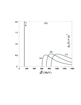
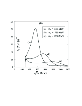
Instead of (iii), one may adopt (the peak position of the spectral function in the channel). We take this simplified condition with three possible cases: =550 MeV, 750 MeV and 1000 MeV. 550 MeV and 750 MeV are consistent with recent re-analyses of the - scattering phase shift [22].
We still have a freedom to choose the renormalization point . Instead of trying to determine optimal by the renormalization group equation for the effective potential [23], we take a simple and physical condition ==140 MeV. This choice has two advantages: (a) One-loop pion self-energy vanishes at the tree-mass; , and (b) the spectral function in the channel starts from a correct continuum threshold in the one-loop level. Resultant parameters are summarized in TABLE I.
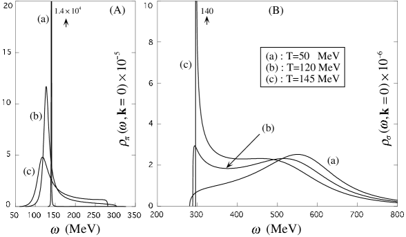
In Fig.3, the spectral functions and at , namely the limit of eq.(38) defined below, are shown as a function of . In the channel, there are one particle pole and a continuum starting from the threshold . is the point where the channel opens. In the channel, the spectral function starts from the threshold MeV and shows a broad peak centered around . The large width of is due to a strong - coupling in the linear model. The corresponding -pole is located far from the real axis on the complex plane.
Here we show the definition of the spectral function at finite :
| (38) |
where is the retarded correlation function
| (39) |
with being the thermal expectation value.
B Application of OPT
Now let us proceed to Step 2 in OPT and rewrite eq.(35) as
| (41) | |||||
Since ( = ) is already a one-loop order, we have neglected the terms proportional to , and which are two-loop or higher orders.
When SSB takes place (), the tree-level masses to be used in the modified loop-expansion read
| (42) |
Since will eventually be a function of , the tree-masses running in the loops are not necessary tachyonic at finite contrary to the naive loop-expansion (see the discussion in Sec. II A).
The thermal effective potential is calculated in the standard manner except for the extra terms proportional to . The effective potential in the one-loop level reads
| (43) | |||||
| (44) | |||||
| (45) |
where . Although this has the similar structure with the standard free energy in the naive loop-expansion, the coefficient of the first term in the r.h.s. of (43) is instead of . This is because we have extra mass-term proportional to in the one-loop level. The stationary point is obtained by
| (46) |
Since the derivative with respect to does not act on , this gives a solution as a function of and . By imposing another condition on (Step 3), one eventually determines both and for given .
C FAC condition for
To resum the hard thermal loops, the PMS condition for the effective potential requires 2-loop calculation, while the FAC condition for the self-energy requires only 1-loop calculation. Therefore, we adopt the latter condition here to determine .
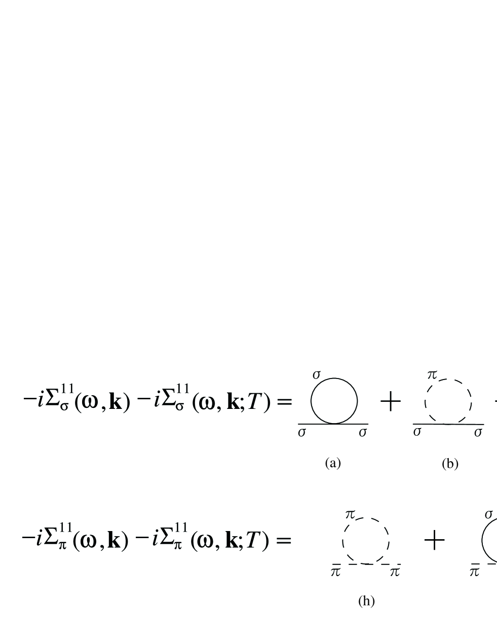
The retarded self-energy (defined by ) is related to the 11-component of the 2 2 self-energy in the real-time formalism [25];
| (47) | |||||
| (48) |
Here is a part having explicit -dependence through the Bose-Einstein distribution, while is a part having only implicit -dependence through and . In the one-loop level, can be calculated only by the 11-component of the free propagator,
| (49) |
with .
One-loop diagrams in OPT for are shown in Fig. 4. Their explicit forms are given in [6]. The NG theorem discussed in Sec. II E can be explicitly checked by comparing eq.(46) and the inverse pion-propagator at zero momentum .
Let us impose the FAC condition on . Since we chose a renormalization condition MeV at zero , one may be tempted to adopt the following condition at finite :
| (50) |
However, eq.(50) does not guarantees that is real, since the l.h.s. of eq.(50) receives an imaginary part due to the Landau damping. To avoid this problem, we take a hybrid condition:
| (51) |
Note that the external energy is set to be zero in the -dependent part.†††Eq. (51) can be formulated in a covariant way by introducing the four-vector characterizing the heat bath. The first term of the equation is only a function of because it is independent. The second term is a function of and . Therefore, the condition reads Because the second term in the l.h.s. vanishes at , the solution of eq.(51) at becomes
| (52) |
Therefore, the FAC condition (51) does not spoil the naive-loop expansion at .
At high (), the following analytic solution is obtained as far as ;
| (53) |
which implies that the Debye screening mass at high is properly taken into account. For realistic values of in TABLE I, the condition is not well satisfied and eq.(51) should be solved numerically.
For intermediate values of , eq.(51) can effectively sum not only the contributions from the diagrams in Fig.4, but also from those in Fig.4. Thus, OPT can go beyond the cactus approximation which sums only the diagrams in Fig.4.
Two remarks are in order here.
- (i)
-
(ii)
In ref.[18], it has been studied the convergence properties of the free energy at high with a variational condition equivalent to the PMS condition here. Although the approach has a problem of renormalization as we have already mentioned, the result is suggestive in the sense that the optimized loop expansion has much better convergence properties than the loop expansion based on the hard thermal loops [26]. Better understanding of the convergence properties both in PMS and FAC conditions is an important future problem.
D Behavior of , and
In Fig.5(A) the tree-level masses in eq.(42) and are shown for MeV. is not tachyonic and approaches to in the symmetric phase. This confirms that our resummation procedure cures the problem of tachyons in Sec. II A.
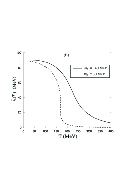
The solid line in Fig.5(B) shows the chiral condensate obtained by minimizing the effective potential with MeV. decreases uniformly as increases, which is a typical behavior of the chiral order parameter at finite away from the chiral limit.
As we approach the chiral limit ( or equivalently ), develops multiple solutions for given , which could be an indication of the first order transition. The critical value of the quark mass below which the multiple solutions arise is
| (54) |
where we have used Gell-Mann-Oakes-Renner relation [27] to related the pion mass with the quark mass. is the physical light-quark mass corresponding to MeV. The critical temperature for is MeV. The behavior of for MeV (just below the critical value ) is also shown by the dashed line in Fig.5(B) for comparison.
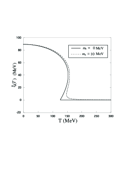
E Chiral limit
In Fig.6 the chiral condensates are shown for the chiral limit ( MeV) and for MeV. The phase transition looks like a first order in these cases. The existence of the multiple solutions of the gap equation for the model in the mean-field approach has been known for a long time [28]. Our analyses confirm this feature within the framework of OPT.
However, this first order nature is likely to be an artifact of the mean-field approach as discussed in the second reference in [28]: the higher loops of massless and almost massless are not negligible near the critical point, and they could easily change the order of the transition. In fact, the renormalization group analyses as well as the direct numerical simulation on the lattice indicate that the model has a second order phase transition [29].
We have also studied the free energy as a function of near the chiral limit and found that it has a discontinuity near the critical point. This is another sign that the first-order nature is an artifact of the approximation. (Remember that, the free energy must be a continuous function of irrespective of the order of the phase transition.)
F Spectral function at finite
As one of the non-trivial applications of OPT, we show, in Fig.7, the spectral functions of and at finite defined in (38) .
The figure shows that the spectral function of , which does not show a clear resonance at , develops a sharp enhancement near 2 threshold as approaches . This is due to a combined effect of the partial restoration of chiral symmetry and the strong coupling. This is an typical example of the softening (or the precursor of the critical fluctuation) associated with the partial restoration of chiral symmetry [30]. The experimental relevance of this softening has been examined in the context of the low-mass diphoton production [6].
In the -channel, a continuum develops by the scattering with thermal pions in the heat-bath; . Because of this process, the pion acquires a width at MeV, while the peak position does not show appreciable modification. They are in accordance with the Nambu-Goldstone nature of the pion.
IV Summary
We have shown that the optimized perturbation theory (OPT) developed in [6] naturally cures the problems of the naive loop-expansion at finite , namely, the breakdown of the naive perturbation at (due to the hard thermal loops) as well as at (due to the tachyonic poles).
Furthermore, OPT has several advantages over other resummation methods proposed so far:
First of all, the renormalization of the UV divergences, which is not a trivial issue in other methods, can be carried out systematically in the loop-expansion in OPT. This is because one can separate the self-consistent procedure (Step 3 in Sec. II C) from the renormalization procedure (Step 2 in Sec. II C).
Secondly, the Nambu-Goldstone (NG) theorem is fulfilled in any give order of the loop-expansion in OPT for arbitrary in theory. This is because OPT preserves the global symmetry of the effective potential in each order of the perturbation.
There are many directions where OPT at finite may be applied. The phase transition in theory as well as the dynamical critical phenomena near the critical point are one of the most interesting problems to be examined further. The PMS condition for the effective action will be suitable for this purpose. OPT may also have relevance to develop an improved perturbation theory for gauge theories in which the weak coupling expansion is known to break down in high orders [31].
Acknowledgments
This work was partially supported by the Grants-in-Aid of the Japanese Ministry of Education, Science and Culture (No. 06102004). S. C. would like to thank the Japan Society of Promotion of Science (JSPS) for financial support.
REFERENCES
- [1]
- [2] E. Braaten and R. D. Pisarski, Nucl. Phys. B337, 569 (1990); ibid. B339, 310 (1990). R. R. Parwani Phys. Rev. D45, 4695 (1992). P. Arnold and C-X. Zhai, Phys. Rev. D50, 7603 (1994); ibid. D51, 1906 (1995).
- [3] S. Weinberg, Phys. Rev. D9, 3357 (1974). L. Dolan and R. Jackiw, Phys. Rev. D9, 3320 (1974).
- [4] G. Baym and G. Grinstein, Phys. Rev. D15, 2897 (1977). H. E. Haber and H. A. Weldon, Phys. Rev. D25, 502 (1982). G. Amelino-Camelia and S-Y. Pi, Phys. Rev. D47, 2356 (1993). G. Amelino-Camelia, Nucl. Phys. B476, 255 (1996); Phys. Lett. B407, 268 (1997). H-S. Roh and T. Matsui, Eur. Phys. J. A1, 205 (1998).
- [5] See, A. Okopińska, Phys. Lett. B375, 213 (1996); A. Dmitrainović, J. A. McNeil and J. R. Shepard, Z. Phys. C69, 359 (1996); G. Amelino-Camelia, Phys. Lett. B407, 268 (1997), and references therein.
- [6] The present article is partially based on the following paper; S. Chiku and T. Hatsuda, Phys. Rev. D58, 076001 (1998), (hep-ph/9803226). See alo, S. Chiku and T. Hatsuda, Phys. Rev. D57, R6 (1998).
- [7] See the review, T. Hatsuda and T. Kunihiro, Phys. Rep. 247, 221 (1994).
- [8] T. Hatsuda, T. Kunihiro and T. Tanaka, Phys. Rev. Lett. 78, 3229 (1997). See also, G. A. Arteca, F. M. Fernández and E. A. Castro, Large Order Perturbation Theory and Summation Methods in Quantum Mechanics, (Springer-Verlag, Berlin, 1990). H. Kleinert, Path Integrals in Quantum Mechanics, Statistical and Polymer Physics, 2nd. edition (World Scientific, Singapore, 1995), Section 5.
- [9] A. Okopińska, Phys. Rev. D36, 2415 (1987); Mod. Phys. Lett. A12, 1003 (1997). (In the first reference, OPT at finite was examined with being a small perturbation, which is in contrast with our approach.) See also, G. A. Hajj and P. M. Stevenson, Phys. Rev. D37, 413 (1988).
- [10] N. Banerjee and S. Mallik, Phys. Rev. D43, 3368 (1991).
- [11] D. A. Kirzhnits and A. D. Linde, Ann. Phys. 101, 195 (1976).
- [12] H. Matsumoto, I. Ojima and H. Umezawa, Ann. Phys. 152, 348 (1984). A. J. Niemi and G. W. Semenoff, Nucl. Phys. B230 [FS10], 181 (1984), and references therein.
- [13] B. W. Lee, Nucl. Phys. B9, 649 (1969). B. W. Lee, Chiral Dynamics, (Gordon and Breach, New York, 1972).
- [14] T. Kugo, Prog Theor. Phys. 57, 593 (1977).
- [15] This point was first recognized in [10].
- [16] P. M. Stevenson, Phys. Rev. D23, 2916 (1981).
- [17] See, e.g. C. Itzykson and J-B. Zuber, Quantum Field Theory, (McGraw-Hill, New York, 1985). T. Muta, Foundations of Quantum Chromodynamics, (World Scientific, Singapore, 1998).
- [18] F. Karsch, A. Patkos and P. Petreczky, Phys. Lett. B401, 69 (1997).
- [19] W. A. Bardeen and M. Mosche, Phys. Rev. D28, 1372 (1983).
- [20] L. H. Chan and R. W. Haymaker, Phys. Rev. D7, 402 (1973); ibid. D10, 4170 (1974).
- [21] R. D. Pisarski and F. Wilczek, Phys. Rev. D29, 338 (1984). K. Rajagopal and F. Wilczek, Nucl. Phys. B399, 395 (1993). M. Asakawa, Z. Huang and X.-N. Wang, Phys. Rev. Lett. 74, 3126 (1995). J. Randrup, Phys. Rev. D55, 1188 (1997) and references therein.
- [22] N. A. Törnqvist and M. Roos, Phys. Rev. Lett. 76, 1575 (1996). M. Harada, F. Sannino and J. Schechter, Phys. Rev. D54, 1991 (1996). S. Ishida et al., Prog. Theor. Phys. 98, 1005 (1997). J. A. Oller, E. Oset and J. R. Peláez, Phys. Rev. Lett. 80, 3452 (1998). K. Igi and K. Hikasa, hep-ph/9807326 (1998).
- [23] M. Bando, T. Kugo, N. Maekawa and H. Nakano, Phys. Lett. B301, 83 (1993).
- [24] J. M. Luttinger and J. C. Ward, Phys. Rev. 118, 1417 (1960). See, also the contributions of J.Knoll, Yu. B. Ivanov and D. N. Voskresenski, hep-ph/9809419 and H. Schulz, hep-ph/9808339 at this conference.
- [25] M. Le Bellac, Thermal Field Theory, (Cambridge Univ. Press, Cambridge, 1996).
- [26] In this conference, related contributions are S. Leupold, hep-ph/9808424 and A. Rebhan, hep-ph/9808480. The former argues the convergence properties in theory, especially, large and case. The later discusses it of the pressure in the large and models.
- [27] M. Gell-Mann, R. J. Oakes and B. Renner, Phys. Rev. 175, 2195 (1968).
- [28] D. A. Kirzhnits and A. D. Linde, Ann. Phys. 101, 195 (1976). G. Baym and G. Grinstein, Phys. Rev. D15, 2897 (1977).
- [29] See, K. Kanaya and S. Kaya, Phys. Rev. D51, 2404 (1995) and references therein.
- [30] T. Hatsuda and T. Kunihiro, Phys. Rev. Lett. 55, 158 (1985); Phys. Lett. B185, 304 (1987). See also, H. A. Weldon, Phys. Lett. B274, 133 (1992); S. Huang and M. Lissia, Phys. Rev. Phys. Rev. D53, 7270 (1996); C. Song and V. Koch, Phys. Lett. B404, 1 (1997).
- [31] A. D. Linde, Phys. Lett. 96B, 289 (1980). T. Hatsuda, Phys. Rev. D56, 8111 (1997) and references therein.