Resumming the pressure

Abstract

The convergence properties of the resummed thermal perturbation series for the thermodynamic pressure are investigated by comparison with the exact results obtained in large-$N$ $\phi^{4}$ theory and possibilities for improvements are discussed. By going beyond conventional resummed perturbation theory, renormalization has to be carried out nonperturbatively yet consistently. This is exemplified in large-$N$ $\phi^{4}_{4}$ and in a special large-$N$ $\phi^{3}_{6}$ model that mimics QED in the limit of large flavour number.

I Introduction

A few years ago, the authors of Ref. [1] have accomplished the task of calculating all contributions to the thermodynamic pressure in QCD that are accessible to conventional resummed perturbation theory, that is up to contributions from the nonperturbative magnetic sector which involve at least $g^{6}$. Dismayingly, the apparent convergence of the perturbation series up to order $g^{5}$, rendered in Fig. 1a, proved to be too poor to warrant its usage at realistic couplings $g\approx 2$. In fact, the convergence is spoiled in particular by the contributions involving resummation effects, as can be seen in Fig. 1a from the large jumps whenever a new contribution involving odd powers in $g$ is included.

Since this problem arises already before one has to face the nonperturbative nature of the (chromo)magnetostatic sector, which contributes to $O(g^{6}T^{4})$, it may have to do with the constraint inherent in perturbation theory to truncate everything to finite-order polynomials in the coupling (up to possible logarithms). This is necessary in view of the needs of the renormalization process, but it certainly discards a large portion of the resummation effects which are in principle contained in low-order diagrams.

The replacement of truncated perturbation series by Padé approximants, i.e. by perturbatively equivalent rational functions, as proposed in Ref. [2] can be considered as a very simple guess what the discarded terms may have been. At any rate, it gives a rough idea as to their importance. In Fig. 1b the result for the pressure is transformed by appropriate Padé approximations, and it does have a big effect for larger coupling. The apparent convergence is somewhat improved, but at $g\approx 2$ the result is still inconclusive; actually, the final result including the 5th order contributions looks even worse than before as it tends to values larger than the free-pressure one.

(a)

(b)

FIG. 1.: a) The perturbative results for the pressure of QCD($N_{f}=3$) up to order $g^{5}$ (full line). Short, medium, and long dashes give the results up to $g^{2}$, $g^{3}$, and $g^{4}$, respectively. b) The corresponding Padé approximants $[0,2]$, $[1,2]$, $[2,2]$, and $[3,2]$.

In this talk, I shall discuss the convergence properties of resummed thermal perturbation theory in simple solvable but nontrivial cases. The starting point will be an exact nonperturbative formula for the full pressure which itself has the form of a one-loop integral. Its evaluation and renormalization will be carried out first in the large-$N$ limit of scalar $\phi^{4}$-theory, which is simplified by the fact that the self-energy is momentum-independent, and then in a special large-$N$ $\phi^{3}_{6}$ model that mimics QED in the limit of large flavour number, which brings in some of the complications coming from momentum-dependent self-energies. Moreover, these toy models have some noteworthy features which also make them interesting on their own.

II A one-loop formula for the nonperturbative pressure

In Ref. [3] we found that at the cost of introducing a further integration with respect to the bare masses of a field theoretical model the full thermodynamic pressure can be expressed as a one-loop integral involving the full self-energy. This follows from the observation that

$${\partial\over\partial m_{0}^{2}}P(T)={1\over i\beta V}\left\langle{1\over 2}\int_{C}d^{4}x\phi^{2}(x)\right\rangle=-{1\over 2}\langle\phi^{2}(0)\rangle$$ (1)

where $C$ is the Keldysh contour of real-time finite-temperature field theory [4], and from the requirement that the pressure $P(T)-P(0)\to 0$ when all masses are sent to infinity. Thus

$$P(T)-P(0)={1\over 2}\int_{m_{0}^{2}}^{\infty}dm_{0}^{\prime 2}\langle\phi^{2}(0)\rangle_{T,m_{0}^{\prime}}-\biggl{(}T=0\biggr{)}$$ (2)

$$={1\over 2}\int_{m_{0}^{2}}^{\infty}dm_{0}^{\prime 2}\int{d^{n}q\over(2\pi)^{n}}\left[D^{12}_{T}(q;m^{\prime}_{0})-D^{12}_{0}(q;m^{\prime}_{0})\right]$$ (3)

$$=-{1\over 2}\int_{m_{0}^{2}}^{\infty}dm_{0}^{\prime 2}{\rm Im}\int{d^{n}q\over(2\pi)^{n}}\biggl{\{}{1+2n(q^{0})\over q^{2}-m_{0}^{\prime 2}-\Pi_{T}(q^{0},{\bf q}^{2};m_{0}^{\prime})}$$ (4)

$$\qquad\qquad\qquad\qquad\qquad\qquad-{1\over q^{2}-m_{0}^{\prime 2}-\Pi(q^{2};m_{0}^{\prime})}\biggr{\}}$$ (5)

where $D^{ab}$ denotes the real-time matrix propagator and $\Pi$ is obtained by diagonalization of the self-energy matrix. This can be easily generalized to fermions and in principle even to (gauge-fixed) gauge theories[3]. While it is true that the introduction of auxiliary masses generally spoils both gauge and BRS symmetries, the combinatorics of the loop expansion which is reshuffled by the mass integration in Eq. (2) does not depend on these symmetries. So although their loss would be a high price in intermediate steps, the full integral depends only on the physical masses (which are zero for gauge bosons).

One noteworthy aspect following from the essential one-loop nature of the above (exact) formula is that it appears to be manifestly infrared-finite in all dimensions $n>3$, irrespective of whether or not $\Pi_{T}$ gives rise to screening (or even divergences). So this seems to be a good new starting point for some reorganization of thermal perturbation theory—which would have to see that $\Pi_{T}$ when obtained in some approximation is not expanded out again from the denominator in Eq. (2). Clearly, this would require a correspondingly reorganized renormalization procedure. So far, everything has been written down in terms of unrenormalized quantities only.

III Nonperturbative renormalization in the example of large-$N$ $\phi^{4}_{4}$ theory

The large-$N$ limit of a scalar O($N$) model with interaction Lagrangian

$${\cal L}_{I}=-{\lambda_{0}\over 4!}{3\over N+2}\left(({{\vec{\phi}}}(x))^{2}\right)^{2}$$ (6)

can be solved exactly [8, 10]. It can also be viewed as a certain approximation to ordinary ${\lambda_{0}\over 4!}\phi^{4}$-theory, in which only those diagrams are kept which have a topology that corresponds to the leading term of a $1/N$-expansion. This infinite set of diagrams is alternatively called Hartree-Fock, super-daisy, cactus, or foam [7] diagrams.

In this approximation, the Schwinger-Dyson equation for the self-energy does not involve vertex functions and is given by a one-loop equation. Its renormalization at $T=0$ gives

$$m^{2}=m_{0}^{2}+\lambda_{0}M(m^{2})$$ (7)

with

$$M(m^{2})={1\over 2}\int{d^{n}q\over(2\pi)^{n}}{i\over q^{2}-m^{2}+i\epsilon}$$ (8)

Similarly, coupling constant renormalization is given by

$$\lambda=\lambda_{0}+\lambda_{0}\lambda M^{\prime}(m^{2})$$ (9)

when renormalizing at zero momentum. In four dimensions, this leads to the problem of triviality if one requires both $\lambda_{0}$ and $\lambda$ to be positive, for then $\lambda\to 0$ as $n\to 4$. Keeping $\lambda>0$ is only possible by using a cut-off or by accepting $\lambda_{0}<0$. In the latter case one finds that the scattering amplitude has a tachyonic pole, but this occurs at $s=s_{\rm tach}\approx-m^{2}e^{32\pi^{2}/\lambda}\approx-m^{2}10^{137/\lambda}$, which is exponentially huge for reasonably small coupling. Either way we can accept this theory as an effective theory for momenta and temperatures $\ll\sqrt{s}_{\rm tach}$.

At finite temperature, the Schwinger-Dyson equation leads to a “gap” equation of the form

$$m^{2}+\delta m^{2}=m_{0}^{2}+\lambda_{0}M_{T}(m^{2}+\delta m^{2})$$ (10)

with

$$M_{T}(m^{2})-M(m^{2})\equiv N_{T}(m^{2})$$ (11)

$$=\int{d^{n}q\over(2\pi)^{n}}2\pi\delta^{+}(q^{2}-m^{2}){1\over e^{q^{0}/T}-1}$$ (12)

Elimination of the unrenormalized parameters in favour of the renormalized ones yields

$$\delta m^{2}(m^{2},T)=\lambda[\hat{M}(m^{2},\delta m^{2})+N_{T}(m^{2}+\delta m^{2})]$$ (13)

with

$$\hat{M}(m^{2},\delta m^{2})$$ (14)

$$\quad=M(m^{2}+\delta m^{2})-M(m^{2})-\delta m^{2}M^{\prime}(m^{2})$$ (15)

The function $\hat{M}$ is formally of order $\lambda^{2}$, i.e. of the same order as 3-loop contributions to the pressure, and it has been occasionally missed in the literature [8]. It exhibits a nontrivial interplay of the thermal mass correction $\delta m^{2}$ with the zero-temperature UV-divergent quantities $M(m^{2})$ and $M^{\prime}(m^{2})$ appearing in the counter-terms.

Rewriting also the pressure in terms of renormalized quantities, we arrive at the remarkable formula

$$P(T)-P(0)=\int_{m^{2}}^{\infty}dm^{\prime 2}{\delta m^{2}(m^{\prime 2},T)\over\lambda(m^{\prime 2})}$$ (16)

where $\lambda(m^{\prime 2})$ is a running coupling that is equal to $\lambda$ when $m^{\prime 2}=m^{2}$; $\lambda_{0}$ is kept fixed throughout.

Fortunately, Eq. (16) can be integrated, yielding

$$P(T)-P(0) = P_{T}^{\rm free}(m^{2}+\delta m^{2})+{1\over 2}{(\delta m^{2})^{2}\over\lambda}$$ (18)

$$-\sum_{n=3}^{\infty}{1\over n!}M^{(n-1)}(m^{2})(\delta m^{2})^{n}$$

While the second term on the right-hand-side can be identified as an interaction contribution, the subsequent terms again come from the thermal mass shift in zero-temperature integrals.

While being UV-finite, the above equation becomes IR-divergent when $m\to 0$. This is not a problem specific to finite temperature, but comes from the breakdown of the on-shell renormalization scheme that we have used so far. In the limit $m\to 0$ one can switch to an off-shell ($\overline{\hbox{MS}}$) scheme through

$$\lambda^{-1}=\bar{\lambda}^{-1}+{1\over 32\pi^{2}}\log{\bar{\mu}^{2}\over m^{2}}$$ (19)

which simplifies

$$\hat{M}\to\bar{M}(\bar{\mu}^{2},\delta m^{2})={1\over 32\pi^{2}}\delta m^{2}\;(\log{\delta m^{2}\over\bar{\mu}^{2}}-1)$$ (20)

It is now only a matter of simple numerical integrations to calculate $\delta m^{2}$ and the resulting pressure.

Somewhat surprisingly, there is not one but two solutions for $\delta m^{2}$ for small values of the coupling, and none for $\bar{\lambda}>\bar{\lambda}_{\rm crit}$, whose value depends (in a renormalization-group invariant manner) on the renormalization scale $\bar{\mu}$. However, the higher values of $\delta m^{2}$ that correspond to one and the same $\bar{\lambda}$ are close to the tachyonic scale $\surd{s_{\rm tach}}$ (see Fig. 2), which we have agreed to ignore. In order that $\surd{s_{\rm tach}}$ be exponentially far away, we need $\bar{\lambda}(T)\ll 10^{2}$, which also cuts out the case of no solution for the thermal mass and therefore for the pressure.

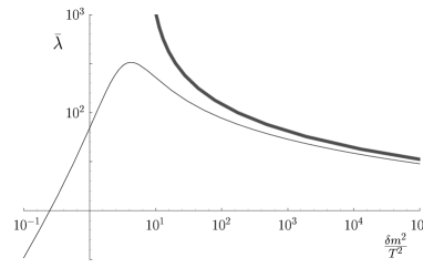
FIG. 2.: The relation between solutions for $\delta m^{2}$ and the renormalized coupling $\bar{\lambda}$; the heavy line marks where $\delta m$ would become equal to the (modulus of the) tachyon mass.

IV Comparison of a nonperturbative result with perturbation series

Besides its pedagogical value, the above nonperturbative result can be put to use to study the properties of (truncated) series expansions in $\bar{\lambda}(\bar{\mu})$. The first few terms in the result for the pressure read

$${P(T)-P(0)\over T^{4}}={\pi^{2}\over 90}-{\bar{\lambda}\over 1152}+{\bar{\lambda}^{3/2}\over 576\pi\sqrt{6}}$$ (21)

$$\qquad\qquad-(6-\gamma-\log{\bar{\mu}\over 4\pi T}){\bar{\lambda}^{2}\over 18432\pi^{2}}$$ (22)

$$\qquad+(3-2\gamma-2\log{\bar{\mu}\over 4\pi T}){\bar{\lambda}^{5/2}\over 12288\pi^{3}\sqrt{6}}$$ (23)

$$\quad-\left((6-\gamma-\log{\bar{\mu}\over 4\pi T})^{2}-30+{\zeta(3)\over 36}\right){\bar{\lambda}^{3}\over 294912\pi^{4}}$$ (24)

$$\qquad\qquad+O(\bar{\lambda}^{7/2})$$ (25)

Comparing truncated series expansions like the above with the full nonperturbative result, we can investigate the convergence properties of an expansion in powers (and logarithms) of $\bar{\lambda}^{1/2}$. It turns out that these depend strongly on the ratio of the arbitrary renormalization scale $\bar{\mu}$ to temperature.

In Fig. 3 we juxtapose the exact and the perturbative result for the pressure $[P(T)-P(0)]$ to its ideal-gas value $\pi^{2}T^{4}/90$, including successively up to 10 terms beyond the leading one. We choose various values of the renormalization scale $\bar{\mu}$, but for ease of comparison in each case we plot against $\bar{\lambda}$ evaluated for $\bar{\mu}=T$.

This shows that when $\bar{\mu}$ is very different from $T$, the convergence of the series deteriorates significantly. For $\bar{\mu}=100T$ (Fig. 3a), the truncated series develop oscillatory behaviour for larger values of the coupling, whereas for $\bar{\mu}={1\over 100}T$, the perturbative results fail to improve with increasing order at roughly the same value of the coupling, albeit in a more peaceful manner. With $\bar{\mu}\approx 2\pi T$, the perturbation series tolerates the largest coupling strength, but it is evident that the perturbative results cannot describe more than a few percent deviation from the free pressure value.

(a)

(b)

FIG. 3.: A comparison of the perturbative results for $\bar{P}\equiv[P(T)-P(0)]/{\pi^{2}T^{4}\over 90}$ as a function of ${\bar{\lambda}^{1/2}(T)}$ up to 12th order for different choices of the renormalization scale: a) $\bar{\mu}=100T$, b) $\bar{\mu}=2\pi T$, c) $\bar{\mu}={1\over 100}T$.

In Fig. 4 the results of a Padé improvement is displayed. This is seen to work surprisingly well except for those cases where the Padé approximant develops a pole beyond which the result appears to be off by a constant.

In QCD, the Padé approximants did not work nearly as well (cf. Fig. 1b). This might have to do with the absence of $\log(\bar{\lambda})$-terms in the large-$N$ limit of our model. In QCD similar logarithmic terms are present and they are treated like constants when building the Padé approximants.

FIG. 4.: As in fig. 3b, but with the perturbative power series replaced by Padé approximants $[0,2]$, $[1,2]$, $[2,2]$, $[2,3],\ldots,[4,4]$. They quickly converge to the exact result with the exception of $[3,3]$, which has a pole.

Let us finally try out a completely different expansion. If we a posteriori expand everything in powers of $\delta m/T$ rather than $\bar{\lambda}$, we find that the convergence properties are excellent so that substantial deviations from the free pressure results can be covered with only a few terms kept (Fig. 5). The reason for this is that the high-temperature expansion has a convergence radius of $\delta m/T=2\pi$, a value which, at least in our model, is always far away for all $\bar{\lambda}\ll\bar{\lambda}_{\rm crit}$.

FIG. 5.: The pressure with solutions of the thermal mass equation truncated at leading order in $\delta m/T$ (top curve) and next-to-leading order (bottom curve). All higher approximations are virtually indistinguishable from the exact solution, and they collectively form the middle line, which broadens only at the highest values of $\bar{\lambda}$.

This, perhaps merely tantalizingly, indicates that a reorganization of thermal perturbation theory as a series in $\delta m/T$ rather than $g$ should lead to dramatic improvements. In this connection see also the proposal of a “screened perturbation theory” in Ref. [12] and the contribution of S. Leupold at this conference [13].

V Nonperturbative renormalization in the example of large-$N$ $\phi^{3}_{6}$ theory

Large-$N$ $\phi^{4}$-theory was exceptionally simple in that the self-energy is momentum independent. In order to learn how to deal with the complications from a momentum-dependent self-energy and the need of wave function renormalization we now consider a scalar $\phi^{3}_{6}$ theory, in which a scalar isovector $A$ is coupled to $N\to\infty$ scalar isodoublets $\psi$ according to [14]

$${\cal L}_{I}=-{g\over\sqrt{N}}A^{a}\psi_{r}^{{\dagger}}\tau^{a}\psi_{r},\qquad r=1,\ldots,N$$ (26)

so that this model mimics large-$N_{f}$ QED, but without the complications of spinor and vector boson fields. The masses of the fields $A$ and $\psi$ are denoted by $m$ and $M$, respectively, and we require $m<2M$ in order to have stable photons.

The same trick as in Sect. 2 can be used to derive a one-loop formula for the full pressure, but it suffices to differentiate and integrate with respect to the “photon” mass $m$, for $m\to\infty$ switches off all interactions. Thus

$$P(T)=P^{\rm free}_{(\psi)}(T,M_{0}^{2})-{3\over 2}{\rm Im}\int_{m_{0}^{2}}^{\infty}dm_{0}^{\prime 2}\int{d^{6-2\epsilon}q\over(2\pi)^{6-2\epsilon}}\biggl{\{}$$ (27)

$$\qquad{1+2n(q^{0})\over q^{2}-m_{0}^{\prime 2}-g_{0}^{2}\pi_{T}(q^{0},{\bf q}^{2})}-{1\over q^{2}-m_{0}^{\prime 2}-g_{0}^{2}\pi(q^{2})}\biggr{\}}$$ (28)

where $\pi_{T}(q^{0},{\bf q}^{2})$ and $\pi(q^{2})$ are the finite-temperature and zero-temperature photon self-energies (with two powers of the coupling factored out), respectively.

In the limit of $N\to\infty$, the interaction pressure is of order $N^{0}$, and to this order there are no corrections to the internal “electron” lines in the one-loop photon self-energy, because the electron self-energy is of order $N^{-1}$. So the latter can be ignored except in $P^{\rm free}_{(\psi)}(T,M_{0}^{2})\sim N$, where the renormalization of $M_{0}$ contributes to the interaction pressure, and is in fact essential to make the latter finite.

The UV divergences in $\pi(q^{2})$ have to be eliminated by mass and wave-function renormalization. Choosing on-shell renormalization we have

$$m^{\prime 2} = m_{0}^{\prime 2}+g_{0}^{2}\pi(m^{\prime 2})$$ (29)

$$g^{2}(m^{\prime 2}) = Z_{2}(m^{\prime 2})g_{0}^{2}$$ (30)

$$Z_{2}(m^{\prime 2}) = {1\over 1-g_{0}^{2}\pi^{\prime}(m^{\prime 2})}={\partial m^{\prime 2}\over\partial m_{0}^{\prime 2}}$$ (31)

$$\bar{\pi}(q^{2}) = \pi(q^{2})-\pi(m^{\prime 2})-(q^{2}-m^{\prime 2})\pi^{\prime}(m^{\prime 2})$$ (32)

$$\bar{\pi}_{T}(q^{0},{\bf q}^{2}) = \pi_{T}(q^{0},{\bf q}^{2})-\pi(m^{\prime 2})-(q^{2}-m^{\prime 2})\pi^{\prime}(m^{\prime 2})$$ (33)

In Eq. (27) the mass integration can be carried out, which is trivial before renormalization and only slightly less so after, with the result

$$P(T)^{\rm int}\equiv P(T)-P(T)\Big{|}_{g=0}$$ (34)

$$\quad=-{3\over 2}{\rm Im}\int{d^{6}q\over(2\pi)^{6}}\biggl{[}2n(q^{0})\log{g^{2}\bar{\pi}_{T}(q^{0},{\bf q}^{2})+m^{2}-q^{2}\over m^{2}-q^{2}}$$ (35)

$$\quad\qquad\qquad\qquad\qquad+\log{g^{2}\bar{\pi}_{T}(q^{0},{\bf q}^{2})+m^{2}-q^{2}\over g^{2}\bar{\pi}(q^{2})+m^{2}-q^{2}}$$ (36)

$$\quad\qquad\qquad\qquad\qquad-{g^{2}\hat{\pi}_{T}(q^{0},{\bf q}^{2})\over g^{2}\bar{\pi}(q^{2})+m^{2}-q^{2}}\biggr{]}$$ (37)

The last term in the square brackets comes from $P^{\rm free}_{(\psi)}(T,M_{0}^{2})-P^{\rm free}_{(\psi)}(T,M^{2})$ and is necessary to remove the UV divergence contained in the second term. There is a subtlety involved here in that $\hat{\pi}\equiv\bar{\pi}_{T}-\bar{\pi}$ except for spacelike momenta; for those this equality holds for the real parts only, while the imaginary parts differ by contributions that vanish exponentially in the ultraviolet. This again provides an example of a nontrivial effect of zero-temperature renormalization in thermal quantities.

Beyond the large-$N$ limit, the renormalization of Eq. (27) becomes much more involved and requires a careful treatment of overlapping divergences, see Ref. [14].

In the large-$N$ limit, we had to consider only one-loop (but this time non-local!) contributions to the self-energies—still, Eq. (34) is clearly a nonperturbative result involving arbitrarily high powers of $g$.

It is in fact a result which could not have been obtained by the methods of hard-thermal-loop resummation. The hard-thermal-loop approximation to $\pi_{T}$ turns out to be identical in form to the longitudinal component of $\Pi_{\mu\nu}^{\rm HTL}$ in four-dimensional gauge theories, but with a reversed over-all sign:

$$\bar{\pi}_{T}^{\rm HTL}(q^{0},{\bf q}^{2})=$$ (38)

$$\qquad\qquad-{T^{2}\over 24\pi}\left(1-{q_{0}^{2}\over{\bf q}^{2}}\right)\left[1-{q_{0}\over 2|{\bf q}|}\log{q_{0}+|{\bf q}|\over q_{0}-|{\bf q}|}\right]$$ (39)

At $q^{0}$ this leads to a screening mass squared with a wrong sign, giving rise to a spacelike pole in the hard-thermal-loop resummed propagator. This has been noted before in $\phi^{3}_{6}$-theories [15], and it is similar to what occurs in the hard-thermal-loop graviton propagator when evaluated (inconsistently) on flat space[16], where this is interpreted as the Jeans instability of a gravitating medium.

In our scalar case, it is a reflection of the unboundedness of the potential from below. For small temperatures, the mass term for the photon stabilizes the system, but thermal mass corrections lead to a diminished total mass up to a point $T=T_{\rm crit}$ where the screening mass vanishes. Beyond this point, an instability develops, because thermal fluctuations become able to surmount the barrier provided by the zero-temperature mass term in the potential, and this is reflected by the appearance of a “tachyonic” screening mass (Fig. 6).

Correspondingly, the pressure (34) is well-defined and real only for $T\leq T_{\rm crit}$. A hard-thermal-loop approximation fails because it approaches the problem from the wrong “side”.

FIG. 6.: The location of poles in the “photon” propagator for $g=10$ at $T=m=m_{1}=m_{2}$ (a), which is below the critical temperature, and at $T=1.5m$ (b), which is above it. The two dashed lines mark the light cone and the zero-temperature mass hyperboloid $q_{0}^{2}={\bf q}^{2}+m_{2}^{2}$. The line between them is the location of the poles in the thermal propagator. In (b) the second full line below the light cone marks zeros of the real part of the inverse propagator, which correspond to poles of the propagator only at its intersections with $q_{0}=0$ because of large Landau damping for $q_{0}>0$ and $q^{2}<0$.

On the other hand, the full nonperturbative $N\to\infty$ result (34) can be evaluated numerically (if tediously) by a couple of nested numerical integrations ($\pi_{T}$ cannot be expressed in terms of elementary functions, but has a rather involved analytic structure).

In Fig. 7, the results of such a numerical evaluation is given for three values of the coupling $g$ and $m=M$, and it is compared with the strictly perturbative $g^{2}$-part of the potential (without hard-thermal-loop resummation).

The nonperturbative pressure exists up to the point $T=T_{\rm crit}\approx\sqrt{24\pi}m/g$. Presumably there is a finite but complex analytic continuation beyond this point, but our derivation is in terms of a manifestly real quantity, which becomes infrared singular for $T>T_{\rm crit}$. Right at the critical temperature, however, where (34) is still well-defined, we are as close as possible to the behaviour of four-dimensional gauge theories in that there is a vanishing screening mass, as is the case for magnetostatic modes in QED.

FIG. 7.: Numerical evaluation of the interaction pressure (34) for three values of $g$ in comparison with the leading perturbative contribution.

VI Conclusion

At least as concerns the thermodynamic pressure of hot QCD, conventional (hard-thermal-loop) resummed perturbation theory, even after including everything that can be treated perturbatively, falls fails to give reliable results for moderately large coupling. The perturbative series shows a surprisingly poor apparent convergence, far worse than usually the case for the range of coupling considered, with the consequence that only a few percent of deviation from the ideal-gas result can be described.

It could well be that this bad behaviour comes from a certain incompleteness of the resummation of hard thermal loops, because finally everything has to be broken down to a truncated series, that is, a polynomial in $g$ and $\log(g)$.

Padé approximants are the simplest possibility to replace the latter by functions that are more likely to fit the actual behaviour at larger values of $g$, but in QCD they only lead to a marginal improvement, if any.

In order to help prepare the (uncertain) way to alternative resummation schemes, we have considered simple scalar theories. Going beyond a strictly perturbative scheme in the coupling involves a correspondingly nonperturbative renormalization. In the simple models that we have considered we have demonstrated the importance of a consistent renormalization scheme.

In large-$N$ $\phi^{4}$ theories we have been able to compare thoroughly the convergence behaviour of an expansion in the coupling with the full nonperturbative result. We have seen the importance of the choice of renormalization scale, but have found that the convergence of these expansions is limited to small coupling and that the range of the latter increases rather slowly with the order of perturbation theory. In contrast to QCD, Padé approximants worked surprisingly well, but this may be specific to the model considered, for which the pressure fortuitously did not involve logarithms in the coupling constant. An exceedingly good approximation was obtained by an expansion in terms of $\delta m/T$ in place of $g$, but it is of course totally unclear how to implement such a scheme in more complicated theories.

REFERENCES

-
[1]
P. Arnold
and C. Zhai, Phys. Rev. D50 (1994) 7603; D51 (1995) 1906;
C. Zhai and B. Kastening, Phys. Rev. D52 (1995) 7232;
E. Braaten and A. Nieto, Phys. Rev. Lett. 76 (1996) 1417; Phys. Rev. D53 (1996) 3421 -
[2]
B. Kastening, Phys. Rev. D56 (1997) 8107;
T. Hatsuda, Phys. Rev. D56 (1997) 8111 - [3] I. T. Drummond, R. R. Horgan, P. V. Landshoff and A. Rebhan, Phys. Lett. B398 (1997) 326
- [4] M. Le Bellac, Thermal Field Theory (Cambridge Univ. Press, Cambridge, 1996)
- [5] P. V. Landshoff, hep-ph/9808362
-
[6]
C. Wetterich, Phys. Lett. B301 (1993) 90;
M. Bonini, M. D’Attanasio and G. Marchesini, Nucl. Phys. B409 (1993) 441 - [7] I. T. Drummond, R. R. Horgan, P. V. Landshoff and A. Rebhan, Nucl. Phys. B524 (1998) 579
- [8] L. Dolan and R. Jackiw, Phys. Rev. D9 (1974) 3320
-
[9]
G. Amelino-Camelia and S.-Y. Pi, Phys. Rev. D47 (1993) 2356;
G. Amelino-Camelia, Phys. Lett. B407 (1997) 268 - [10] W. A. Bardeen and M. Moshe, Phys. Rev. D28 (1983) 1372
- [11] R. R. Parwani and H. Singh, Phys. Rev. D51 (1995) 4518
- [12] F. Karsch, A. Patkós and P. Petreczky, Phys. Lett. B401 (1997) 69
- [13] S. Leupold, hep-ph/9808424
- [14] D. Bödeker, P. V. Landshoff, O. Nachtmann and A. Rebhan, hep-ph/9806514
- [15] R. D. Pisarski, Nucl. Phys. A525 (1991) 175c
-
[16]
D. J. Gross, M. J. Perry and L. G. Yaffe, Phys. Rev. D25 (1982) 330;
P. S. Gribovsky, J. F. Donoghue and B. R. Holstein, Ann. Phys. (NY) 190 (1989) 149;
A. Rebhan, Nucl. Phys. B351 (1991) 706