Extraction method of $\gamma$ from semi-inclusive $b\rightarrow Ds$ decays

Ji-Ho Jang ***e-mailΒ :Β jhjang@chep6.kaist.ac.kr Department of Physics, Korea Advanced Institute of Science and Technology,
Taejon 305-701, Korea
Abstract

We propose a new method to extract a $CP$ angle $\gamma$ from semi-inclusive two-body nonleptonic decays, $b\rightarrow D^{0}(\bar{D}^{0})s$ and $b\rightarrow D_{CP}s$. This method is free from the unknown long distance strong interaction effects and gives theoretically cleaner signal than the similar method using exclusive nonleptonic decays, $B\rightarrow DK$. We can determine $\gamma$ with 4-$\sigma$ accuracy for $40^{o}\lesssim\gamma\lesssim 160^{o}$.

††preprint: August, 1998 KAIST-16/98 hep-ph/9808478

In the standard model ( SM ), the source of $CP$ asymmetry is one complex phase in the Cabibbo-Kobayashi-Maskawa ( $CKM$ ) matrix element [1]. Until now, only one experimental evidence of $CP$ violation is found in $K_{L}\rightarrow\pi\pi$ decay and it comes dominantly from $K^{0}-\bar{K}^{0}$ mixing. Hence it should be important to probe the $CP$ violation in the $B$ systems in the future experiment in order to test the SM scenario of $CP$ violation. One of the important objects to investigate $CP$ violation is the unitary triangle which includes three angles $\alpha,\beta$ and $\gamma$. The angles $\beta$ and $\gamma$ are related to $V_{td}$ and $V_{ub}$ respectively and the angle $\alpha$ is obtained using the unitary relation $\alpha+\beta+\gamma=\pi$. The recent numerical constraints of the three angles are given [2] :

$\displaystyle-1.0\leq$ $\displaystyle\sin 2\alpha$ $\displaystyle~{}\leq 1.0,$ (1)
$\displaystyle 0.30\leq$ $\displaystyle\sin 2\beta$ $\displaystyle~{}\leq 0.88,$ (2)
$\displaystyle 0.27\leq$ $\displaystyle\sin^{2}\gamma$ $\displaystyle~{}\leq 1.0.$ (3)

There are many suggestions to determine independently the angles of the unitary triangle. For example, the angle $\alpha$ can be determined by $B\rightarrow\pi\pi$ modes if their gluonic penguin pollutions can be removed using the isospin relation [3]. The $B\rightarrow J/\psi K_{S}$ decay is gold-plated mode to determine the angle $\beta$ because the $CKM$ angles from decay processes are almost canceled in the rate asymmetry and it can be unambiguously determined by $B^{0}-\bar{B}^{0}$ mixing which is related to the angle $\beta$. The angle $\gamma$ may be obtained by $B\rightarrow DK$ modes [4, 5]. But it is noted in [6] that this method has the experimental difficulties because the final $\bar{D}^{0}$ meson should be identified using $\bar{D}^{0}\rightarrow K^{+}\pi^{-}$, but it is difficult to distinguish it from doubly Cabibbo suppressed $D^{0}\rightarrow K^{+}\pi^{-}$ following color and $CKM$ allowed $B^{-}\rightarrow D^{0}K^{-}$. There are some variant methods to overcome these difficulties [6, 7, 8, 9]. In Ref.[6], the interference between $B^{-}\rightarrow D^{0}[\rightarrow\pi^{-}K^{+}]K^{-}$ decay and $B^{-}\rightarrow\bar{D}^{0}[\rightarrow\pi^{-}K^{+}]K^{-}$ decay is used. The extraction method of the angle $\gamma$ using the color-allowed decays only is proposed in Ref.[7]. In Ref. [8, 9], authors proposed the extraction method of $\gamma$ using the isospin relation and neglecting the annihilation diagrams.

Other methods to constrain the angle $\gamma$ from $B\rightarrow K\pi$ modes has been also proposed in Ref.[10]. However the long distance strong interaction effects might destroy the validity of this method [11]. These uncertainties and electro-weak penguin pollutions can be removed by using the $B\rightarrow KK$ modes and $SU(3)$ flavor symmetry [12]. Such rescattering effects may be potentially important in any exclusive decays of $B$ meson decays and it is important to remove hadronic uncertainties coming from the rescattering effects.

It is noted by several authors that inclusive and semi-inclusive decays of $B$ meson could show large $CP$ violation [14, 15, 16]. In Ref.Β [14], the authors estimate the rate asymmetry using the absorptive part of the decay amplitude. Gerard and Hou [14] noted that $CPT$ theorem is violated if one does not include all diagrams of the same order. The $CP$ violation in the semi-inclusive charmless, single charm and double charm transition is considered in Ref.Β [15]. Moreover as the large cancellation between the semi-inclusive decay rates, the $CP$ violation effects in the totally inclusive decays are expected to be tiny. However one can expect the large $CP$ violation in the each of the semi-inclusive decays. Authors in Ref.Β [16] investigate the $CP$ violation in the quasi-inclusive decays of the type $B\rightarrow K^{(*)}X$ that the strange quark is only included in $K^{(*)}$ meson. The interference between the tree level process $b\rightarrow u\bar{u}s$ and the one loop process bβ†’s​gβˆ—β†’s​q​q¯→𝑏𝑠superscriptπ‘”β†’π‘ π‘žΒ―π‘žb\rightarrow sg^{*}\rightarrow sq\bar{q} gives the direct $CP$ violation.

In the Ref.[13], authors proposed a systematic method of experimental search for two-body hadronic decays of the $b$-quark of the type bβ†’q​u​a​r​k​(q)+m​e​s​o​n​(M)β†’π‘π‘žπ‘’π‘Žπ‘Ÿπ‘˜π‘žπ‘šπ‘’π‘ π‘œπ‘›π‘€b\rightarrow quark(q)+meson(M). They have the well-defined experimental signature because the spectrum of the meson energy should be a peak centered around $(m_{b}^{2}+m_{M}^{2}-m_{q}^{2})/2m_{b}$ with a spread of a few hundred MeV. The energy of outgoing quark will be similar to that of the meson and become $\sim 2$ GeV numerically. The hadronization process of the quark will lead to low average multiplicity about 3/event. They insisted that the combinatorics problem in discriminating against background is not so difficult. They considered the tree$\times$penguin and penguin$\times$penguin type processes to estimate the partial rate asymmetries and to consider electroweak penguin dominated branching ratios.

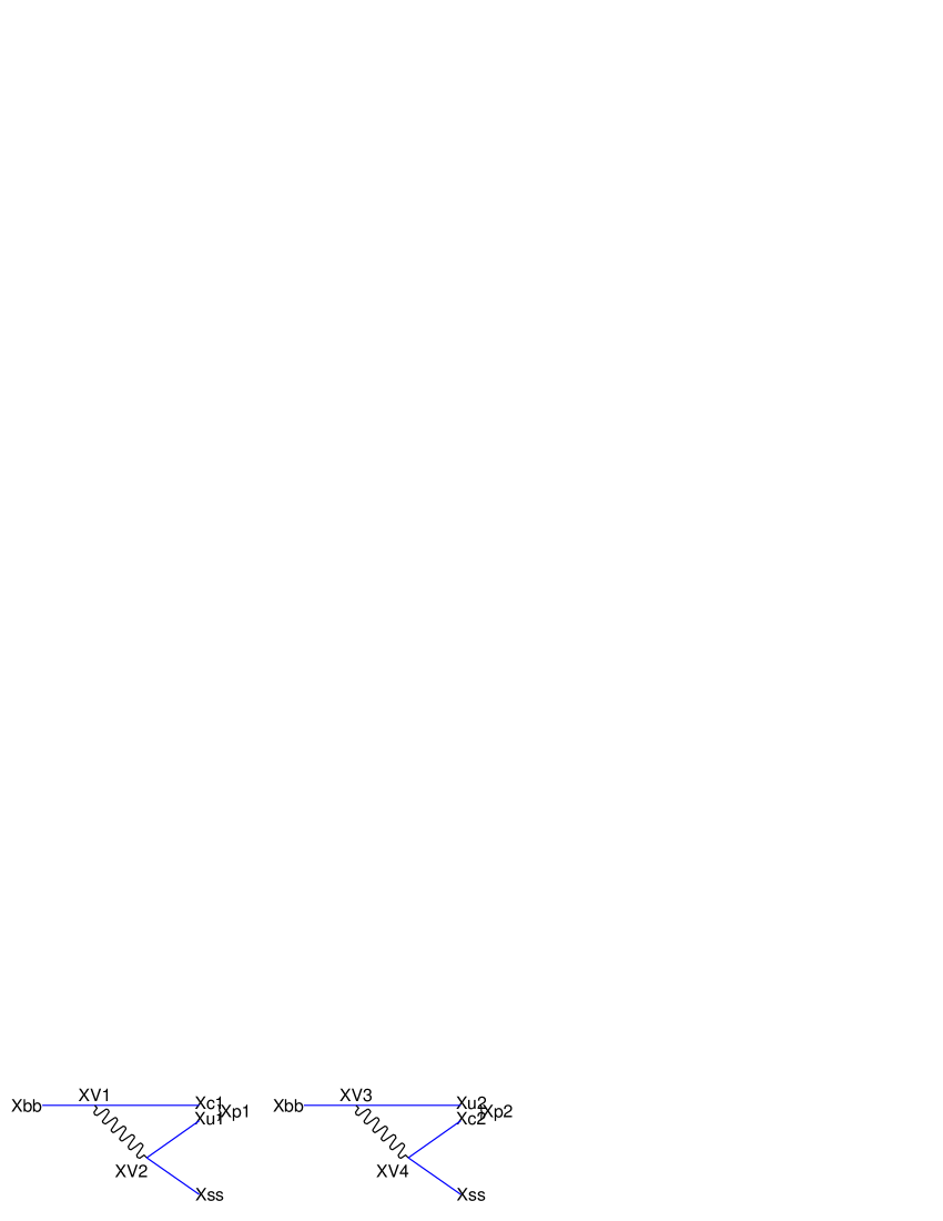
In this letter, we suggest a new extraction method of $\gamma$ using the semi-inclusive two-body decays of the type $b\rightarrow D^{0}(\bar{D}^{0})s$ and $b\rightarrow D_{CP}s$ which come form only tree diagrams ( see Fig.Β 1 ). These modes have the same advantage as other semi-inclusive decays given in Ref.Β [13]. The theoretical values of the decay rates would be less uncertain than the exclusive modes because the hadronic form factors are replaced with the calculation of quark diagrams. As these decay modes are semi-inclusive processes and final states involve a kind of isospin state, we also expect that they are free from the long distance effects of strong interaction. Because we consider decays of $b-$quark, all kinds of $B$ hadrons can be used in this analysis.

The effective Hamiltonian relevant to $b\rightarrow Ds$ decays is given by

$\displaystyle{\cal H}_{eff}$ $\displaystyle=$ $\displaystyle-\frac{G_{F}}{\sqrt{2}}\left[V_{cb}V^{*}_{us}\left\{c_{1}(\bar{s}u)_{V-A}(\bar{c}b)_{V-A}+c_{2}(\bar{c}u)_{V-A}(\bar{s}b)_{V-A}\right\}\right.$ (5)
$\displaystyle~{}~{}~{}~{}+\left.V_{ub}V^{*}_{cs}\left\{c_{1}(\bar{s}c)_{V-A}(\bar{u}b)_{V-A}+c_{2}(\bar{u}c)_{V-A}(\bar{s}b)_{V-A}\right\}+h.c.\right],$

where $c_{1(2)}$ are the Wilson coefficients and the subindex $V-A$ denotes $\gamma_{\mu}(1-\gamma_{5})$ structure.

Let us introduce the relevant amplitudes as follows,

$\displaystyle A(b\rightarrow D^{0}s)=$ $\displaystyle A(\bar{b}\rightarrow\bar{D}^{0}\bar{s})$ $\displaystyle~{}={\cal A},$ (6)
$\displaystyle e^{i\gamma}A(b\rightarrow\bar{D}^{0}s)=$ $\displaystyle e^{-i\gamma}A(\bar{b}\rightarrow D^{0}\bar{s})$ $\displaystyle~{}={\cal A}~{}R_{b},$ (7)

where $R_{b}=\sqrt{\rho^{2}+\eta^{2}}=0.36\pm 0.08$. The initial state $b(\bar{b})$ is isosiglet and the final states are isodoublet. Hence these processes are described by the effective Hamiltonian of $|\Delta I|=1/2$ and all amplitudes are given by the a complex number ${\cal A}$ with same strong phases and different $CKM$ factors. It is a main advantage of using these semi-inclusive decays that there is no relative strong phase in the above amplitudes.

The semi-inclusive decay rates into flavor specific states of $D$ meson are given by

$\displaystyle\Gamma(b\rightarrow D^{0}s)=$ $\displaystyle\Gamma(\bar{b}\rightarrow\bar{D}^{0}\bar{s})$ $\displaystyle~{}=\left|{\cal A}\right|^{2}~{}F_{P.S},$ (8)
$\displaystyle\Gamma(b\rightarrow\bar{D}^{0}s)=$ $\displaystyle\Gamma(\bar{b}\rightarrow D^{0}\bar{s})$ $\displaystyle~{}=\left|{\cal A}\right|^{2}~{}R_{b}^{2}~{}F_{P.S},$ (9)

where $F_{P.S.}$ is phase space factor and we neglect the small phase space differences.

On the other hand, using the definition of $CP$ eigenstates of $D$ mesons, $D_{1(2)}=\frac{1}{\sqrt{2}}(D^{0}\pm\bar{D}^{0})$, and neglecting the small $D^{0}-\bar{D}^{0}$ mixing, we obtain the decay rates into $CP$ eigenstate of final $D$ meson:

$\displaystyle\Gamma(b\rightarrow D_{1}s)=$ $\displaystyle\Gamma(\bar{b}\rightarrow D_{1}\bar{s})$ $\displaystyle~{}=\frac{1}{2}~{}\left|{\cal A}\right|^{2}~{}F_{P.S.}~{}(1+R_{b}^{2}+2R_{b}\cos\gamma),$ (10)
$\displaystyle\Gamma(b\rightarrow D_{2}s)=$ $\displaystyle\Gamma(\bar{b}\rightarrow D_{2}\bar{s})$ $\displaystyle~{}=\frac{1}{2}~{}\left|{\cal A}\right|^{2}~{}F_{P.S.}~{}(1+R_{b}^{2}-2R_{b}\cos\gamma).$ (11)

Decay rate ratios ${\cal A}_{i}$ between $CP$ eigenstates and flavor specific states in the final $D$ mesons are defined as follows,

$\displaystyle{\cal A}_{i}$ $\displaystyle=$ $\displaystyle\frac{\Gamma(b\rightarrow D_{i}s)+\Gamma(\bar{b}\rightarrow D_{i}\bar{s})}{\Gamma(b\rightarrow D_{1}s)+\Gamma(\bar{b}\rightarrow D_{1}\bar{s})+\Gamma(b\rightarrow D_{2}s)+\Gamma(\bar{b}\rightarrow D_{2}\bar{s})}$ (12)
$\displaystyle=$ $\displaystyle\frac{\Gamma(b\rightarrow D_{i}s)+\Gamma(\bar{b}\rightarrow D_{i}\bar{s})}{\Gamma(b\rightarrow D^{0}s)+\Gamma(\bar{b}\rightarrow\bar{D}^{0}\bar{s})+\Gamma(b\rightarrow\bar{D}^{0}s)+\Gamma(\bar{b}\rightarrow D^{0}\bar{s})},$ (13)

where $i=1,2$ is $CP$-even and odd eigenstates respectively and in the second line, we use the following relation coming from Eq.Β (8) and (10) :

$\displaystyle\Gamma(b\rightarrow D^{0}s)+\Gamma(\bar{b}\rightarrow\bar{D}^{0}\bar{s})+\Gamma(b\rightarrow\bar{D}^{0}s)+\Gamma(\bar{b}\rightarrow D^{0}\bar{s})$ (14)
$\displaystyle=$ $\displaystyle\Gamma(b\rightarrow D_{1}s)+\Gamma(\bar{b}\rightarrow D_{1}\bar{s})+\Gamma(b\rightarrow D_{2}s)+\Gamma(\bar{b}\rightarrow D_{2}\bar{s}).$ (15)

Using Eq.(8), we can simplify the ratio ${\cal A}_{i}$ as follows,

$${\cal A}_{i}=\frac{1}{2}\pm\frac{R_{b}}{1+R_{b}^{2}}\cos\gamma,$$ (16)

where $\pm$ correspond to $i=1,2$ respectively. Note that these simple relations come from the fact that there is no relative strong phase between $A(b\rightarrow D^{0}s)$ and $A(b\rightarrow\bar{D}^{0}s)$ in Eq.Β (6).

We can also define a combined asymmetry ${\cal R}$ between $CP$-even and odd states as follows,

$\displaystyle{\cal R}$ $\displaystyle=$ $\displaystyle{\cal A}_{1}-{\cal A}_{2}$ (17)
$\displaystyle=$ $\displaystyle\frac{\{\Gamma(b\rightarrow D_{1}s)+\Gamma(\bar{b}\rightarrow D_{1}\bar{s})\}-\{\Gamma(b\rightarrow D_{2}s)+\Gamma(\bar{b}\rightarrow D_{2}\bar{s})\}}{\{\Gamma(b\rightarrow D_{1}s)+\Gamma(\bar{b}\rightarrow D_{1}\bar{s})\}+\{\Gamma(b\rightarrow D_{2}s)+\Gamma(\bar{b}\rightarrow D_{2}\bar{s})\}},$ (18)

Using Eq.(10) or Eq(16), $\cos\gamma$ is related to the asymmetry ${\cal R}$ as

$$\cos\gamma=\frac{{\cal R}(1+R_{b}^{2})}{2R_{b}}.$$ (19)

The sum of initial $b$ and $\bar{b}$ states is used in the definition of the ratio ${\cal A}_{i}$ in Eq.Β (12) and the asymmetry ${\cal R}$ in Eq.Β (17). Hence there is no need tagging of the initial $b$ and $\bar{b}$ states and it is an experimental advantage of this method.

From Eq.Β (16), (19) and using the present experimental value of $R_{b}=0.36\pm 0.08$, we can obtain the bound of the ratios ${\cal A}_{i}$ and the asymmetry ${\cal R}$ :

$\displaystyle 0.18\leq$ $\displaystyle{\cal A}_{i}$ $\displaystyle\leq 0.82,$ (20)
$\displaystyle-0.64\leq$ $\displaystyle{\cal R}$ $\displaystyle\leq 0.64.$ (21)

If the ratios ${\cal A}_{i}$ and ${\cal R}$ are determined between the above range in the future experiments, we can constrain the angle $\gamma$ using the experimental data.

Let’s probe the feasibility of this method in determining the angle $\gamma$. We need to know the branching ratio of each mode and the detection efficiences. In order to estimate the branching ratio of the relevant decay, we use the factorization approximation and obtain the relevant transition amplitudes :

$\displaystyle A(b\rightarrow D^{0}s)$ $\displaystyle=$ $\displaystyle\frac{G_{F}}{\sqrt{2}}~{}V_{cb}V^{*}_{us}~{}a_{2}<D^{0}|\bar{c}u_{-}|0><s|\bar{s}b_{-}|b>,$ (22)
$\displaystyle A(b\rightarrow\bar{D}^{0}s)$ $\displaystyle=$ $\displaystyle\frac{G_{F}}{\sqrt{2}}~{}V_{ub}V^{*}_{cs}~{}a_{2}<\bar{D}^{0}|\bar{u}c_{-}|0><s|\bar{s}b_{-}|b>,$ (23)

where $a_{2}=c_{2}+c_{1}/N_{c}$ and $\bar{q}q^{\prime}_{-}=\bar{q}\gamma_{\mu}(1-\gamma_{5})q^{\prime}$.

The branching ratio is given by

$\displaystyle Br(b\rightarrow D^{0}s)=\left|\frac{V_{cb}V^{*}_{us}}{V_{ub}V^{*}_{cs}}\right|^{2}Br(b\rightarrow\bar{D}^{0}s)$ (24)
$\displaystyle=\frac{G_{F}^{2}}{8\pi m_{b}}~{}|V_{cb}V^{*}_{us}|^{2}~{}a_{2}^{2}~{}f_{D}^{2}~{}R~{}\tau_{b}~{}[2(p_{s}\cdot p_{D})(p_{b}\cdot p_{D})-(p_{s}\cdot p_{b})m_{D}^{2}]$ (25)
$\displaystyle\simeq 0.67\times 10^{-4},$ (26)

where $R=(1+R_{1}^{2}+R_{2}^{2}-2R_{1}R_{2}-2R_{1}-2R_{2})^{1/2}$ with R1=(ms/mb)2subscript𝑅1superscriptsubscriptπ‘šπ‘ subscriptπ‘šπ‘2R_{1}=(m_{s}/m_{b})^{2} and $R_{2}=(m_{D}/m_{b})^{2}$. In this numerical calculation, we use the following parameter set : $\tau_{b}=1.55\times 10^{-12}$sec, a2=0.21,fD=200​M​e​V,ms=120​M​e​V,mD=1.87​G​e​Vformulae-sequencesubscriptπ‘Ž20.21formulae-sequencesubscript𝑓𝐷200𝑀𝑒𝑉formulae-sequencesubscriptπ‘šπ‘ 120𝑀𝑒𝑉subscriptπ‘šπ·1.87𝐺𝑒𝑉a_{2}=0.21,f_{D}=200~{}MeV,m_{s}=120~{}MeV,m_{D}=1.87~{}GeV and $m_{b}=4.8~{}GeV$. The values of the branching ratios depend on the specific parameter set, the factorization assumption and the Fermi motion of the $b$-quark in the $B$ mesons. However the above typical values are enough to estimate the errors in determining the $\gamma$.

In order to estimate the uncertainty in the determination of the angle $\gamma$, we assume $3\times 10^{8}$ $B\bar{B}$ events in $B$ factories using $e^{+}e^{-}$ annihilation at the $\Upsilon(4S)$ resonance. Tagging of $D^{0}(\bar{D}^{0})$ is used $D^{0}\rightarrow K^{-}\pi^{+},D^{0}\rightarrow K^{-}\pi^{+}\pi^{+}\pi^{-}$ and $D^{0}\rightarrow K^{-}\pi^{+}\pi^{0}$ modes and its total efficiency is about $0.25$. The $CP$ even-state $D_{1}$ is identified by $D_{1}\rightarrow\pi^{+}\pi^{-},K^{+}K^{-}$ and the observation rate is $5\times 10^{-2}$ which is quoted in Ref. [5]. The tagging of $CP$ odd state $D_{2}$ uses the $D_{2}\rightarrow K_{s}\pi^{+}\pi^{-}$ whose branching ratio is $5.4\%$. The observation rate is $3.6\%$ as $K_{S}$ is identified by $K_{S}\rightarrow\pi^{+}\pi^{-}$ mode whose branching fraction is about 2/3.

The number of the observable events can be obtained by the product of the number of the $B\bar{B}$ event, the branching ratio of the each modes and the detection efficiencies of the final particles. The statistical error in the branching ratio is approximately given by $\Delta Br/Br\approx 1/\sqrt{N_{\rm obs}}$. The numerical values of the statistical error become about $1.4\%$ and $3.9\%$ for $b(\bar{b})\rightarrow D^{0}s(\bar{D}^{0}\bar{s})$ and $b(\bar{b})\rightarrow\bar{D}^{0}s(D^{0}\bar{s})$, respectively. For the modes with $CP$ eigen states in the final states, the values depend on the angle $\gamma$. Presenting the values in order of $b\rightarrow D_{1}s(\bar{b}\rightarrow D_{1}\bar{s})$ and $b\rightarrow D_{2}s(\bar{b}\rightarrow D_{2}\bar{s})$, they become $3.4\%(4.0\%)$ and $6.3\%(7.4\%)$ for $\gamma=30^{o}$, $4.0\%(4.7\%)$ and $4.4\%(5.2\%)$ for $\gamma=80^{o}$ and $5.9\%(6.9\%)$ and $3.4\%(4.0\%)$ for $\gamma=140^{o}$, respectively.

Using this information, we can estimate the error in determining $\gamma$. The result is given in Fig.Β 2, where the horizontal and vertical axis represent $\gamma$ and $\Delta\gamma$ in degrees, respectively. The real line and dashed line present the error in $\gamma$ determined using the ratio ${\cal A}_{1}$ and ${\cal A}_{2}$. The dotted line is error plot using the combined asymmetry ${\cal R}$. They all give the similar results. From $40^{o}$ to $160^{o}$, we can determine $\gamma$ with $4$-$\sigma$ accuracy. We also investigate the possibility to extarct the information of the angle $\gamma$ in the smaller number of $B\bar{B}$ events, $3\times 10^{7}$. The result is given in Fig.Β 3. Even in this case, our method may give the reliable results that the angle can be determined with 2-$\sigma$ accuracy for $40^{o}\lesssim\gamma\lesssim 60^{o}$ and 3-$\sigma$ accuracy for $60^{o}\lesssim\gamma\lesssim 160^{o}$.

In conclusion, we proposed a new extraction method of $\gamma$ using the semi-inclusive decays of the type $b\rightarrow Ds,\bar{D}s,D_{CP}s$. These decays are relevant to only tree diagram (Fig.Β 1) and there is no relative strong phase depending on the final states because the final states are related to the semi-inclusive modes and only one kind of isospin state. Then we can simply relate $\cos\gamma$ to the $R_{b}$ and the ratios ${\cal A}_{i},{\cal R}$ which should be determined in future experiment. Since we consider decays of $b-$quark, all kinds of $b-$ hadrons can be used in this analysis. We also probe the feasibility of the suggested method in this paper by estimating the statistical errors in determination of the angle $\gamma$ which is given in Fig.Β 2. The value of $\gamma$ should be determined with $4$-$\sigma$ accuracy for $40^{o}\lesssim\gamma\lesssim 160^{o}$ using $3\times 10^{8}B\bar{B}$ events in our method.

Acknowledgements.
I am grateful to Prof. Pyungwon Ko for helpful discussions, encouragement and reading the manuscript.

REFERENCES

  • [1] N. Cabibbo, Phys. Rev. Lett. 10 (1963) 531; M. Kobayash and K. Maskawa, Prog. Theor. Phys. 49 (1973) 652.
  • [2] A. J. Buras, TUM-HEP-299-97, hep-ph/9711217 ; J.L. Rosner, Nucl. Instrum. Meth. A 408, 308 (1998) ; A. Ali, hep-ph/9801270.
  • [3] M. Gronau and D. London, Phys. Rev. Lett. 65 (1990) 3381.
  • [4] M. Gronau and D. London, Phys. Lett. B253 (1991) 483; M. Gronau and D. Wyler, Phys. Lett. B265 (1991) 172.
  • [5] I. Dunietz, Phys. Lett. B270 (1991) 75.
  • [6] D. Atwood, I. Dunietz and A. Soni, Phys. Rev. Lett. 28 (1997) 3257.
  • [7] M. Gronau, CALT-68-2159, hep-ph/9802315.
  • [8] M. Gronau and J. L. Rosner, EFI-98-29, FERMILAB-PUB-98-227-T, hep-ph/ 9807447.
  • [9] J. H. Jang and P. Ko, KAIST-14/98, SNUTP 98-079, hep-ph/9807469.
  • [10] R. Fleischer and T. Mannel, Phys. Rev. D57 (1998) 2752.
  • [11] J. M. Gerard and J. Weyers, UCL-IPT-97-18, hep-ph/9711469; M. Neubert, Phys. Lett. B424 (1998) 152; A. F. Falk, A. L. Kagan, Y. Nir and A. A. Petrov, Phys. Rev. D57 (1998) 4290; D. Atwood and A. Soni, AMES-HET-97-10, hep-ph/9712287.
  • [12] R. Fleischer, CERN-TH/98-60, hep-ph/9802433; CERN-TH/98-128, hep-ph/9804319; M. Gronau and J. L. Rosner, EFI-98-23, hep-ph/9806348.
  • [13] D. Atwood and A. Soni, AMES-HET-98-6,BNL-HET-98/19, hep-ph/9805393.
  • [14] M. Bander, D. Siverman and A. Soni, Phys. Rev. Lett. 43 (1979) 242; J. M. Gerard and W. S. Hou, Phys. Rev. D43 (1991) 2909; H. Simma, G. Eilam and D. Wyler, Nucl. Phys. B352 (1991) 367; L. Wolfenstein, Phys. Rev. D43 (1991) 151; A. Lenz, U. Nierste and G. Ostermaier, DESY-97-208, hep-ph/9802202.
  • [15] I. Dunietz, FERMILAB-PUB-97/323-T, hep-ph/9806521; M. Beneke, G. Buchalla and I. Dunietz, Phys. Lett. B393 (1997) 132; J. Bernabeu and C. Jarlskog $ibid.$ B301 (1993) 273; I. Dunietz and R. G. Sachs, Phys. Rev. D37 (1988) 3186; (E) $ibid.$ D39 (1989) 3515.
  • [16] T. T. Browder, A. Datta, X. G. He and S. Pakvasa, hep-ph/9807280; Phys. Rev. D57 (1998) 6829.

Refer to caption

FIG. 1.: Feynman diagram for $b\rightarrow Ds$ decay modes

Refer to caption

FIG. 2.: The $\Delta\gamma$ ( error ) plot in the determination of $\gamma$ assuming $3\times 10^{8}$ $B$’s at $B$ factories : real line is using $A_{1}$, dashed line is using $A_{2}$ and dotted line is using $R$

Refer to caption

FIG. 3.: The $\Delta\gamma$ ( error ) plot in the determination of $\gamma$ assuming $3\times 10^{7}$ $B$’s at $B$ factories : real line is using $A_{1}$, dashed line is using $A_{2}$ and dotted line is using $R$