Numerical Toy-Model Calculation of the Nucleon Spin Autocorrelation Function
in a Supernova Core

Abstract

We develop a simple model for the evolution of a nucleon spin in a hot and dense nuclear medium. A given nucleon is limited to one-dimensional motion in a distribution of external, spin-dependent scattering potentials. We calculate the nucleon spin autocorrelation function numerically for a variety of potential densities and distributions which are meant to bracket realistic conditions in a supernova core. For all plausible configurations the width $\Gamma$ of the spin-density structure function is found to be less than the temperature $T$. This is in contrast with a naive perturbative calculation based on the one-pion exchange potential which overestimates $\Gamma$ and thus suggests a large suppression of the neutrino opacities by nucleon spin fluctuations. Our results suggest that it may be justified to neglect the collisional broadening of the spin-density structure function for the purpose of estimating the neutrino opacities in the deep inner core of a supernova. On the other hand, we find no indication that processes such as axion or neutrino pair emission, which depend on nucleon spin fluctuations, are substantially suppressed beyond the multiple-scattering effect already discussed in the literature. Aside from these practical conclusions, our model reveals a number of interesting and unexpected insights. For example, the spin-relaxation rate saturates with increasing potential strength only if bound states are not allowed to form by including a repulsive core. There is no saturation with increasing density of scattering potentials until localized eigenstates of energy begin to form.

]

I Introduction

The numerical modeling of stellar collapse and supernova explosions has enjoyed enormous progress which is not quite matched by the poor development of the microscopic input physics. This unsatisfactory state of affairs has recently motivated a number of authors [1, 2, 3] to turn their efforts toward a better understanding of one particular key ingredient, the neutrino opacities in a hot and dense nuclear medium, for which only crude prescriptions have thus far been used in supernova codes. The emphasis of these works has been to address the composition dependence of the opacities (hyperons may be important), and to include many-body effects which range from Pauli phase-space blocking over the inclusion of modified nucleon dispersion relations to “screening,” i.e. nucleon-nucleon correlations.

We study a further aspect of in-medium neutrino reaction rates which was not mentioned in these papers, the topic of nucleon multiple-scattering effects. Their possible importance derives from the observation that the scattering of neutrinos on nonrelativistic nucleons is dominated by axial-vector current interactions, i.e. it is primarily a spin-dependent phenomenon. The nucleon-nucleon interaction contains a strong spin-dependent piece, leading to a large nucleon spin-fluctuation rate in a hot nuclear medium. In the nonrelativistic limit, these spin fluctuations are the sole microscopic source for the emission of neutrino pairs or axions from a supernova core or a neutron star [4, 5], processes which are perturbatively described as nucleonic bremsstrahlung. Moreover, spin fluctuations inevitably lead to a reduction of the neutrino-nucleon interaction rate [6, 7] and to an increase of the energy transfer rate between the neutrino and nucleon fluids [5, 8].

The key quantity for our discussion is the rate $\Gamma$ of spontaneous nucleon spin fluctuations, or equivalently, the rate by which a nuclear spin in the medium loses memory of its orientation. Of course, this process is described by a single constant $\Gamma$ only if the polarization of a given spin decays exponentially as $e^{-\Gamma t}$; in general the temporal evolution of the spin autocorrelation is more complicated.

A perturbative calculation of, say, neutrino pair emission as a bremsstrahlung process $NN\to NN\nu\bar{\nu}$ by virtue of a one-pion exchange potential implies a value for $\Gamma$ much larger than a typical temperature $T$ of a supernova core. On the other hand, the resulting suppression of the neutrino opacities is in blunt conflict with the large duration of the SN 1987A neutrino signal unless one discards as background all of the late-time events [9]. It was thus concluded that the true $\Gamma$ in a real SN core is probably not much larger than $T$. Additional theoretical support for this empirical conclusion arose from a modified $f$-sum rule for the spin-density structure function which was derived by one of us [10].

We presently study a one-dimensional toy model for the nucleon spin relaxation in a “background medium” of spin-dependent potentials. We believe that our model captures the essential physics of the nucleon spin evolution, yet is simple enough to allow for an intuitive understanding and a numerical non-perturbative treatment. The conclusion will be that for plausible configurations of density and potential strengths we always have $\Gamma\lesssim T$, suggesting that multiple-scattering effects are indeed not a dominating feature of the neutrino opacities in the deep inner core of a supernova. Of course, it also means that the rates for axion or neutrino pair emission are much smaller than given by a naive bremsstrahlung treatment. Ironically, then, precisely because perturbation theory is bad in a SN core implies that a naive calculation of $\nu N$ scattering, ignoring nucleon spin fluctuations, is a much better approximation than it deserves!

In Sec. II we describe and justify the physical structure of our model. In Sec. III we discuss our technique for the numerical calculation of the spin-density structure function. Sec. IV is devoted to numerical results, and in Sec. V we conclude with a discussion and summary. We use natural units, $\hbar=c=k_{B}=1$, throughout.

II Model

A Spin-Density Structure Function

As a starting point for our model construction we consider a nonrelativistic single-species medium consisting of nucleons $N$. In this case the main quantity of interest for neutrino opacities and axion emissivities is the positive definite spin-density structure function

$$S(\omega,{\bf k})=\int_{-\infty}^{+\infty}dt\,e^{i\omega t}\,R(t,{\bf k}).$$ (1)

It is the Fourier transform of the normalized spin auto-correlation function

$$R(t,{\bf k})\equiv\frac{4}{3n_{N}}\langle\hat{\hbox{\boldmath$\sigma$}}(t,{\bf k})\cdot\hat{\hbox{\boldmath$\sigma$}}(0,-{\bf k})\rangle,$$ (2)

where $\hat{\hbox{\boldmath$\sigma$}}(x)=\frac{1}{2}\psi^{\dagger}(x){\hbox{\boldmath$\sigma$}}\psi(x)$ is the spin-density operator with $\psi(x)$ the nonrelativistic nucleon field operator, a Pauli two-spinor, while $\sigma$ is the vector of Pauli matrices. Further, $n_{N}$ is the nucleon number density and $\langle\cdots\rangle$ denotes a thermal ensemble average. The normalization factor is given by $\langle\hat{\hbox{\boldmath$\sigma$}}(0,{\bf k})\cdot\hat{\hbox{\boldmath$\sigma$}}(0,-{\bf k})\rangle=s(s+1)\,n_{N}$ for all ${\bf k}$ with $s=\frac{1}{2}$ the length of the spin. Therefore, if the nucleon spins are uncorrelated with each other we have $R(0,{\bf k})=1$, corresponding to

$$\int_{-\infty}^{+\infty}\frac{d\omega}{2\pi}\,S(\omega,{\bf k})=1.$$ (3)

We are primarily interested in the relaxation behavior of $R(t,{\bf k})$. Therefore, we may equally imagine that possible correlation effects are absorbed in the definition of $R$ so that $R(0,{\bf k})=1$ can be imposed as a normalization condition.

While $S(\omega,{\bf k})$ is what appears as a scattering kernel in the Boltzmann collision equation for neutrinos, it is not the most practical quantity for a theoretical discussion. It obeys the principle of detailed balancing,

$$S(-\omega,{\bf k})=e^{-\omega/T}\,S(\omega,{\bf k}),$$ (4)

and thus is not symmetric. Correspondingly, $R(t,{\bf k})$ has a nontrivial imaginary part. However, it is enough to consider a symmetric correlator

$$\bar{R}(t,{\bf k})\equiv\frac{3}{4n_{N}}\,\frac{\left\langle\hat{\hbox{\boldmath$\sigma$}}(t,{\bf k})\cdot\hat{\hbox{\boldmath$\sigma$}}(0,-{\bf k})+\hat{\hbox{\boldmath$\sigma$}}(0,{\bf k})\cdot\hat{\hbox{\boldmath$\sigma$}}(t,-{\bf k})\right\rangle}{2},$$ (5)

which is real because $\bar{R}(t,{\bf k})=\frac{1}{2}[R(t,{\bf k})+R^{*}(t,{\bf k})]=\frac{1}{2}[R(t,{\bf k})+R(-t,{\bf k})]$ and thus is the closest quantum analogue to a classical correlation function. It is equivalent to a structure function which is even in $\omega$,

$$\bar{S}(\omega,{\bf k})=\frac{S(\omega,{\bf k})+S(-\omega,{\bf k})}{2}.$$ (6)

The normalization remains unchanged. We can always recover the scattering kernel by virtue of

$$S(\omega,{\bf k})=\frac{2\bar{S}(\omega,{\bf k})}{1+e^{-\omega/T}},$$ (7)

bringing out detailed balance explicitly.

B Long-Wavelength Limit

In the absence of spin-dependent forces the evolution of the nucleon spins is trivial. In this case the $\omega$-dependence of $\bar{S}(\omega,{\bf k})$ is exclusively caused by nucleon recoils, implying $\bar{S}(\omega,0)=2\pi\delta(\omega)$. For a nonvanishing momentum transfer ${\bf k}$, the width of $\bar{S}$ is given by the nucleon recoil and thus is suppressed by the inverse nucleon mass.

The presence of spin-spin interactions changes this picture in that there will be correlation effects. If we ignore the tensor force as in Ref. [2], the total nucleon spin is still conserved in binary collisions, allowing for spin dissipation only by diffusion. While the structure of $\bar{S}(\omega,{\bf k})$ is now more complicated, it still has nonvanishing power only for $\omega^{2}-{\bf k}^{2}<0$. Put another way, the “screening corrections” of Ref. [2] primarily lead to a reshuffling of the power of $\bar{S}(\omega,{\bf k})$, but it continues to have power only where it has already from recoil effects.

We are primarily interested in the opposite situation, i.e. the effect of the tensor force which allows for local spin dissipation by coupling the nucleon spins to the orbital motion. It creates power in $\bar{S}(\omega,{\bf k})$ for $\omega^{2}-{\bf k}^{2}>0$ and, in particular, has a nonvanishing width even in the long-wavelength limit ${\bf k}\to 0$. Among other consequences this implies that neutrino pairs and axions can be emitted or absorbed, processes which are perturbatively described as bremsstrahlung $NN\leftrightarrow NN\nu\bar{\nu}$. Without the tensor force such processes do not occur as can be shown, for example, by an explicit calculation. The bremsstrahlung picture suggests that $\bar{S}(\omega,{\bf k})$ depends only weakly on ${\bf k}$, essentially because momentum conservation can be achieved among the nucleons alone. Therefore, it is probably enough to develop an understanding of the behavior of the structure function in the long-wavelength limit, $\bar{S}(\omega)=\lim_{{\bf k}\to 0}\bar{S}(\omega,{\bf k})$.

Our simple final approach is, therefore, to study the single-nucleon spin autocorrelation function as a proxy for the collisional broadening of the full dynamical spin-density structure function.

If the effect of collisions on the spin evolution of a given nucleon can be pictured as a sequence of uncorrelated “kicks,” then the autocorrelation function must decay exponentially,

$$\bar{R}(t)=e^{-\Gamma|t|},$$ (8)

where the quantity $\Gamma$ is what we call the spin-fluctuation or spin-relaxation rate. If the spin is completely randomized in a given collision, one can show that $\Gamma$ is identical with the collision rate $\Gamma_{\rm coll}$. The structure function corresponding to Eq. (8) is a Lorentzian,

$$\bar{S}(\omega)=\frac{2\Gamma}{\omega^{2}+\Gamma^{2}}.$$ (9)

A (classical) bremsstrahlung calculation involving single “kicks” yields $\bar{S}(\omega)=2\Gamma/\omega^{2}$. The Lorentzian structure, which we obtain directly from a Fourier transform of Eq. (8), is equivalent to a resummation of a sequence of uncorrelated kicks, i.e. it arises from the multiple-scattering nature of the spin motion caused by a random sequence of collisions.

C Estimate of $\Gamma$

The perturbative estimate of $\Gamma$ is based on a calculation of the bremsstrahlung process $NN\to NN\nu\bar{\nu}$ (Appendix A). Using a one-pion exchange potential and nondegenerate nucleons it is found to be approximately $\Gamma/T=1.24\,\rho_{14}\,T_{30}^{-1/2}$ where $\rho_{14}=\rho/10^{14}~{}{\rm g}~{}{\rm cm}^{-3}$ and $T_{30}=T/30~{}{\rm MeV}$. $\Gamma/T$ of a few is enough to imply a significant neutrino cross-section suppression (Appendix B).

The question if the perturbatively estimated $\Gamma$ is realistic can be addressed by a simple classical estimate. The nucleon spin relaxation is caused by collisions with other nucleons. The most effective relaxation is achieved if the spin is completely randomized in each collision so that $\Gamma=\Gamma_{\rm coll}$. The maximum collision rate, on the other hand, is estimated by the time it takes a given nucleon to cross the average distance to the next scattering center. For nondegenerate nucleons in thermal equilibrium we have $\frac{1}{2}m_{N}v^{2}=\frac{3}{2}T$, leading to a typical velocity of $v=(3T/m_{N})^{1/2}=0.31\,T_{30}^{1/2}$. A typical inverse distance between nucleons is $n_{N}^{1/3}=77.3\,\rho_{14}^{1/3}\,{\rm MeV}$. At this density the pion-fields produced by the nucleons overlap so that the average distance between nucleons should, indeed, represent the distance between scattering events. Therefore, we estimate that the spin-relaxation rate cannot be larger than

$$\frac{\Gamma_{\rm coll}}{T}\approx\frac{n_{N}^{1/3}v}{T}=0.8\,\rho_{14}^{1/3}T_{30}^{-1/2},$$ (10)

an estimate which we think is a generous upper limit because a full spin randomization in each collision is by no means assured. Therefore, the perturbative result looks too large even for a density $10^{14}~{}\rm g~{}cm^{-3}$, not to mention supranuclear densities, and the spin relaxation rate is expected to be significantly smaller than the temperature.

D One-Dimensional Model

The way we performed the classical estimate of the relaxation rate essentially defines our model. We picture the spin to evolve due to spin-dependent potentials which the nucleon encounters as it moves. The spin evolution is thus determined by the potential seen along the nucleon path which we picture as being one-dimensional—the nucleon motion in coordinate space should not have a decisive impact on the (three-dimensional) spin motion.

We are thus led to ask the following question. If we consider a nucleon, constrained to one-dimensional motion, how does the relaxation behavior of the spin depend on the density and strength of the scattering potentials? Can the relaxation rate become as large or even larger than the temperature for configurations which mimic the situation in a supernova core?

To address these questions we calculate the spin correlation function for a nucleon which is confined to a one-dimensional box of length $L$. We place a number of scattering potentials into this box at random locations, calculate numerically the exact $\bar{R}(t)$ or $\bar{S}(\omega)$, and then take an ensemble average over many configurations.

A scattering potential at location $x_{0}$ is taken to interact with the test nucleon according to a Hamiltonian density of the form

$$H_{\rm int}={\hbox{\boldmath$\mu$}}(x-x_{0})\cdot\hat{\hbox{\boldmath$\sigma$}}(x).$$ (11)

The classical “magnetic dipole” is

$${\hbox{\boldmath$\mu$}}(x)={\bf m}\,V(x)$$ (12)

with ${\bf m}$ a unit vector pointing in some random direction while $V(x)$ is a function with the dimension energy. We model it by a Gaussian with

$$V(x)=V_{0}\,e^{-(x/b)^{2}}$$ (13)

where $b$ is a length scale.

In order to avoid bound states we will sometimes add a repulsive diagonal potential so that the total interaction becomes

$$H_{\rm int}=V(x-x_{0})\,\,\frac{1}{2}\psi^{\dagger}(x)({\bf m}\cdot{\hbox{\boldmath$\sigma$}}+1)\psi(x).$$ (14)

For nucleons polarized in the ${\bf m}$-direction this implies that a spin-down neutron feels no potential at all while a spin-up neutron feels twice the (repulsive) potential.

We believe that our approach represents the minimal model that allows one to study the dependence of the relaxation rate on the potential strength and density without recourse to perturbative methods.

III Numerical Technique

A Solving the Schrödinger Equation

For a numerical determination of the spin autocorrelation function we solve explicitly the one-dimensional Schrödinger equation

$$\partial_{t}\left|\psi(x,s_{z},t)\right\rangle=-i\,H\,\left|\psi(x,s_{z},t)\right\rangle,$$ (15)

where $\psi(x,s_{z},t)$ is a nucleon single-particle wavefunction which depends on the one-dimensional coordinate $x$, the $z$-component of the spin $s_{z}=\pm 1/2$, and time $t$. The Hamiltonian is

$$H=-\frac{1}{2m_{N}}\,\frac{\partial^{2}}{\partial x^{2}}+H_{\rm int}.$$ (16)

This partial differential equation is solved by discretizing it on a spatial grid of spacing $a$ so that $x_{j}=j\,a$, $j=1,\cdots,n_{x}$, i.e. the box size is $L=(n_{x}+1)\,a$. We use Dirichlet boundary conditions $\psi(0)=\psi(L)=0$, implying that there are $n_{x}$ grid points where $\psi(x_{j})\not=0$ and thus $n_{x}$ orthonormal states for each $s_{z}=\pm 1$. For the kinetic energy we use the discretized prescription

$$(H_{\rm kin}\psi)(x_{j})=-\frac{\psi(x_{j+1})+\psi(x_{j-1})-2\psi(x_{j})}{2m_{N}a^{2}}.$$ (17)

We then integrate over a time interval $[0,t_{\rm max}]$ in steps of length $dt$.

In practice, at each time step the complex linear equation

$$\left|\psi(t+dt)\right\rangle=\left|\psi(t)\right\rangle+\left(\frac{1-iH\,dt/2}{1+iH\,dt/2}-1\right)\left|\psi(t+dt)\right\rangle$$ (18)

is implicitly solved for $\left|\psi(t+dt)\right\rangle$. This finite-difference representation of $\exp[-iH\,dt]$ is accurate to second order in $dt$ and unitary. Equation (18) is employed alternatingly for the $n_{x}$-dimensional spatial part using $H_{\rm kin}$ for both spin polarizations, and using the two-dimensional spin-dependent part $H_{\rm int}$ at all spatial grid points.

In terms of a complete set of orthonormal functions $|j,s_{z}\rangle$ the correlation function is given by the expression

$$R(t,k)=$$ (19)

$$\Biggl{\langle}\sum_{{j=1,\ldots,n_{x}}\atop{s_{z}=\pm 1/2}}\frac{\langle j,s_{z}|e^{-H/T+iHt+ikx}\sigma_{z}e^{-iHt-ikx}\sigma_{z}|j,s_{z}\rangle}{3Z}\Biggr{\rangle},$$ (20)

where the partition function is

$$Z=\sum_{{j=1,\ldots,n_{x}}\atop{s_{z}=\pm 1/2}}\langle j,s_{z}|e^{-H/T}|j,s_{z}\rangle.$$ (22)

The outer average in Eq. (19) is over many configurations of the scattering potentials.

The scalar products in Eq. (19) can be written as the matrix elements ${}_{A,t}\langle j,s_{z}|e^{ikx}\sigma_{z}|j,s_{z}\rangle_{B,t}$ between the states $|j,s_{z}\rangle_{A,t}\equiv e^{-iHt}e^{-H/T}|j,s_{z}\rangle$ and $|j,s_{z}\rangle_{B,t}\equiv e^{-iHt}e^{-ikx}\sigma_{z}|j,s_{z}\rangle$. Put another way, for a complete set of basis functions $|j,s_{z}\rangle$ we need to solve the Schrödinger equation for the states $e^{-H/T}|j,s_{z}\rangle$ and $e^{-ikx}\sigma_{z}|j,s_{z}\rangle$, respectively, and then take the matrix element of the operator $e^{ikx}\sigma_{z}$.

The runs presented here will always be for the long-wavelength limit with $k=0$. We have verified that $S(\omega,k)$ is indeed nearly independent of $k$ as long as $k\lesssim T$. Furthermore, we will always calculate the symmetric (real) correlator $\bar{R}(t)={\rm Re}\,R(t)$.

B Long-Time Behavior

The numerical solutions for $\bar{R}(t)$ obtained in this way have the somewhat unintuitive property that they relax to a nonvanishing value $\lim_{t\to\infty}\bar{R}(t)=\bar{R}_{\infty}>0$. This long-time behavior is an artifact of the discrete nature of our solution.

This is understood most easily when we write the structure function in terms of the energy eigenstates $|n\rangle$, energy $\omega_{n}$, as

$$S(\omega,{\bf k}) = \frac{8\pi}{n_{N}}\sum_{n,m}\frac{e^{-\omega_{n}/T}\left|\left\langle n|\hat{\hbox{\boldmath$\sigma$}}(0,{\bf k})|m\right\rangle\right|^{2}}{3Z}$$ (24)

$$\hskip 70.0001pt{}\times\delta(\omega+\omega_{n}-\omega_{m}),$$

where $Z=\sum_{n}\langle n|n\rangle\,e^{-\omega_{n}/T}$ is the partition function.

For a finite number of states the weight of the diagonal part of the double sum ($\omega_{n}=\omega_{m}$) does not vanish relative to the nondiagonal part ($\omega_{n}\not=\omega_{m}$). Therefore, $S(\omega,{\bf k})$ inevitably has a nonvanishing amount of power proportional to $\delta(\omega)$ even though its spectrum otherwise is continuous because the ensemble average over different potential configurations washes out the discrete nature of the energy differences $\omega_{n}-\omega_{m}$ for $n\not=m$. The power of $\delta(\omega)$ shows up as a positive constant term in the Fourier transform $\bar{R}(t)$.

C Short-Time Behavior

The relaxation behavior of $\bar{R}(t)$ cannot be exponential at arbitrarily early times, corresponding to arbitrarily large frequencies in Fourier space. Very high frequencies correspond to the (spatial) Fourier components of the scattering potential which is not arbitrarily hard. One expects that the (quantum) structure function has finite moments of the form

$$\int_{-\infty}^{+\infty}\frac{d\omega}{2\pi}\,\omega^{n}\,S(\omega)$$ (25)

for all $n$. (The case $n=1$ is the usual $f$-sum.) They will exist if the potential is infinitely often differentiable everywhere. Assuming that this is the case we conclude that $S(\omega)$ must fall off faster than any power of $\omega$ and that the correlation function can be represented as

$$\bar{R}(t)=1-(\Gamma_{2}t)^{2}+{\cal O}[(\Gamma_{2}t)^{4}],$$ (26)

i.e. it has a vanishing derivative at $t=0$.

D Relaxation Rate

The interpretation of the numerical $\bar{R}(t)$ would be straightforward if it were exactly an exponential decay law, which in general it is not. Therefore, we need a useful prescription to quantify the “relaxation rate,” or equivalently, the “width” of $\bar{S}(\omega)$. Put another way, we need to define what we mean with $\Gamma$ for a non-exponential behavior of $\bar{R}(t)$.

Among many possibilities which differ by a factor of order unity we find it most natural, for the present purposes, to use the neutrino-nucleon cross-section reduction as a starting point. By virtue of Eq. (B9) we can calculate the cross-section suppression from the numerical $\bar{R}(t)$, and then translate it into an equivalent width $\Gamma_{\rm eff}$ of a Lorentzian that would produce the same cross-section reduction. From Fig. 15 we conclude that all of the relevant information of $\bar{R}(t)$ is contained in the time interval $0\leq t\lesssim 2/T$.

E Born Approximation

For sufficiently weak potentials $V(x)$ a perturbative calculation of the structure function can be performed in Born approximation which is a useful test of our numerical code. For the 3-dimensional case and a single scattering center such a comparison has been performed in detail in Ref. [11].

In one dimension for one scattering potential of the form Eq. (11) the spin-density structure function in Born approximation in the long-wavelength limit for $\omega>0$ is

$$S_{\rm Born}(\omega) = \frac{2}{3}\frac{\rho_{\rm s}m_{N}}{\omega^{2}}\int_{0}^{\infty}\!\!dp\,f_{p}\,\frac{\left|\tilde{V}(p_{+})\right|^{2}+\left|\tilde{V}(p_{-})\right|^{2}}{\left(p^{2}+2m_{N}\omega\right)^{1/2}}$$ (28)

$$\hskip 30.00005pt\bigg{/}\int_{0}^{\infty}\!\!dp\,f_{p}$$

where $\tilde{V}(k)\equiv\int_{-\infty}^{+\infty}dx\,e^{-ikx}V(x)$ is the Fourier transform of the potential $V(x)$, $p_{\pm}=(p^{2}+2m_{N}\omega)^{1/2}\pm p$, $f_{p}=e^{-p^{2}/(2m_{N}T)}$ is the nucleon occupation number, and $\rho_{s}$ is the (linear) density of scattering centers. This structure function is not resummed, i.e. it diverges for $\omega\to 0$, as expected for a bremsstrahlung result without including multiple scattering.

For a Gaussian potential of the form Eq. (13) the Born approximation should be valid when

$$|V(x)|\ll\frac{1}{m_{N}b^{2}},\quad\hbox{or}\quad|V(x)|\ll\frac{p}{m_{N}b},$$ (29)

where $p$ is a typical nucleon momentum.

If we take the Gaussian to be very narrow, approaching a $\delta$-function, then the Fourier transform $\tilde{V}$ is a constant and we find

$$S_{\rm Born}^{0}(\omega)=\frac{4(2\pi)^{1/2}}{3}\,\frac{\rho_{s}m_{N}^{1/2}}{T^{1/2}}\,\frac{(V_{0}b)^{2}}{\omega^{2}}\int_{0}^{\infty}\!\!du\,\frac{e^{-u^{2}}}{\sqrt{u^{2}+\omega/T}}.$$ (30)

This expression diverges at $\omega=0$ because it is a first-order un-resummed perturbative result. We can still calculate the neutrino cross-section reduction by virtue of Eq. (B2), which in turn can be translated into an equivalent width $\Gamma_{\rm Born}^{0}$ of a Lorentzian which produces the same cross-section reduction. We find

$$\frac{\Gamma_{\rm Born}^{0}}{T}=C\,\frac{\rho_{s}m_{N}^{1/2}}{T^{3/2}}\,(V_{0}b)^{2}$$ (31)

with

$$C = \frac{4}{3}\int_{0}^{\infty}dx\,\frac{1-(1+x+x^{2}/6)\,e^{-x}}{(2\pi)^{1/2}A\,x^{2}}\int_{0}^{\infty}du\,\frac{e^{-u^{2}}}{\sqrt{u^{2}+x}}$$ (32)

$$= \frac{3\pi^{2}-16}{18\,(2\pi)^{1/2}A}=0.68752,$$ (33)

where the constant $A$ is defined in Eq. (B6).

F Collision Rate

We finally estimate the rate by which a nucleon in our model encounters a scattering potential. If the nucleons are at temperature $T$, their average kinetic energy in one dimension is $\frac{1}{2}m_{N}\langle v^{2}\rangle=\frac{1}{2}T$ so that $\langle v^{2}\rangle=T/m_{N}$. Taking a Maxwellian velocity distribution tells us that $\langle|v|\rangle=(2/\pi)^{1/2}\,\langle v^{2}\rangle^{1/2}$ so that $\langle|v|\rangle=(2T/\pi m_{N})^{1/2}$. If the average (linear) density of scatterers in our model is $\rho_{s}$, then our average collision rate is $\Gamma_{\rm coll}=\langle|v|\rangle\rho_{s}$, or

$$\frac{\Gamma_{\rm coll}}{T}=\left(\frac{2}{\pi Tm_{N}}\right)^{1/2}\,\rho_{s}.$$ (34)

Ultimately, the purpose of our numerical runs is to check if this estimate can be reached, or even surpassed, for a plausible configuration.

IV Numerical Results

A Parameters

We now turn to several series of numerical runs where we have calculated $\bar{R}(t)$. A given run is characterized by the maximum potential strength $V_{0}$ (in MeV) and its width $b$ (in fm) according to Eq. (13) and by whether or not we include a spin-independent repulsive core (RC) to avoid bound states. Further parameters are the temperature $T$ (MeV), the grid spacing $a$ (fm), the density of scatterers $\rho_{s}$ (${\rm fm}^{-1}$), the box size $L$ (fm), the total number of scatterers in the box $n_{s}$, the number of configurations calculated $n_{c}$ so that the statistical significance is proportional to $n_{s}n_{c}$, and finally the integration time $t_{\rm max}$ and the time step $dt$ (both in MeV^-1). We usually take the number of time steps $t_{\rm max}/dt$ to be a power of 2 as required for a numerical cosine transform of $\bar{R}(t)$ to determine $\bar{S}(\omega)$.

As already indicated, the energy unit is MeV, the time unit MeV^-1, and the length unit $1~{}{\rm fm}=(197~{}{\rm MeV})^{-1}$. Note also that the distance between nucleons scales as $n_{N}^{1/3}=77.3\,\rho_{14}^{1/3}\,{\rm MeV}$ and $n_{N}^{-1/3}=2.55\,\rho_{14}^{-1/3}\,{\rm fm}$. We will give all quantities in these units in the remainder of this paper. Most runs presented in the following were performed for $b=1$ and $T=30$, for which Eqs. (28), (B2), and (B5) yield

$$\frac{\Gamma_{\rm Born}}{T}=3.07\times 10^{-4}\,\rho_{s}\,V_{0}^{2}.$$ (35)

Likewise, the estimated collision rate from Eq. (34) is numerically

$$\frac{\Gamma_{\rm coll}}{T}=5.13\,\frac{\rho_{s}}{T^{1/2}}.$$ (36)

These parameters allow one a first estimate of what to expect in a given run.

The required CPU-time scales roughly linearly with the step size $t_{\rm max}/dt$ and with the number of configurations $n_{c}$, but quadratically with the number of grid points $L/a$.

B Born-Approximation Test

In order to test our numerical code we compare the (un-resummed) dynamical structure function in Born approximation of Eq. (28) with the one derived from a numerical run. The characteristic parameters for the run are given in Table I. For these parameters, the condition Eq. (29) would be $V_{0}\lesssim 35$. Further, $\Gamma_{\rm Born}/T=7.67\times 10^{-4}$ and $\Gamma_{\rm coll}/T=0.094$, again implying that a perturbative estimate should be reasonable.

TABLE I.: Parameters for Run Born Test.

$V_{0}$	$b$	RCa	$T$	$\rho_{\rm s}$	$a$	$L$	$t_{\rm max}$	$dt$
5	1	yes	30	0.1	0.7	100	81.92	0.005

^aRepulsive Core in the potential.

In Fig. 1 we compare the numerical $\bar{S}(\omega)$, with the Born approximation $\bar{S}_{\rm Born}(\omega)=S_{\rm Born}(\omega)\,(1+e^{-\omega/T})/2$ where $S_{\rm Born}(\omega)$ is from Eq. (28). In addition, we show the Born approximation $\bar{S}^{0}_{\rm Born}(\omega)$ of Eq. (30) for a $\delta$-function potential with the same $V_{0}b$. The two Born curves differ only for large $\omega$ where the structure of the potential is resolved in a collision. The numerical structure function and the Born approximation agree very well for intermediate frequencies as they should. This agreement is also reflected in the effective spin fluctuation rate, $\Gamma_{\rm eff}=0.0199$, and $\Gamma_{\rm Born}=0.0230$. Note that $\Gamma_{\rm Born}^{0}=0.0487$ is a factor 2.12 larger because a $\delta$-function potential produces more power at large frequencies.

FIG. 1.: Numerical result for $\bar{S}$ of the Born Test run (solid line), as compared to $\bar{S}_{\rm Born}$ (long dashed line). The dotted line is $\bar{S}^{0}_{\rm Born}$, corresponding to a $\delta$-function potential.

C Variation of the Box Size

In Sec. III B we have remarked that the numerical $\bar{R}(t)$ relaxes to a constant value for $t\to\infty$, an effect attributed to the finite box size of our numerical runs. In order to verify that this constant term indeed decreases with increasing box size, we have performed a series of runs Box Size with the characteristics summarized in Table III; there was no repulsive diagonal potential.

TABLE II.: Common parameters for Series Box Size.

$V_{0}$	$b$	RC	$T$	$a$	$\rho_{\rm s}$	$t_{\rm max}$	$dt$
30	1	no	30	1	0.1	32.768	0.002

TABLE III.: Results for Series Box Size.

Runa	$n_{\rm s}$	$n_{\rm c}$	$\bar{R}_{\infty}$	$1/\bar{R}_{\infty}$
B0	1	4096	0.336	2.98
B1	2	2048	0.214	4.67
B2	4	1024	0.157	6.38
B3	8	512	0.127	7.87
B4	16	252	0.105	9.49
B5	32	74	0.104	9.63
B6	64	18	0.090	11.12

^aRun B$n$ has a box size $L=10\times 2^{n}$.

FIG. 2.: Spin autocorrelation function $\bar{R}(t)$ for the Box Size runs B0, B1, B2, B3, B6 (top to bottom).

We show the numerical $\bar{R}(t)$ for several runs in Fig. 2 and summarize the results in Table III. We have calculated the limiting value for $\bar{R}(t)$ as the average of $\bar{R}(t)$ for $20\leq t\leq t_{\rm max}$. It becomes indeed smaller for an increasing box size, but only very slowly. Run B0 with only one scattering center does not relax to a constant at all; the remaining oscillations of $\bar{R}(t)$ signal that “bound-state effects” in the small box are important.

In Fig. 3 we plot $1/\bar{R}_{\infty}$ against $\log_{2}(n_{s})$, revealing an almost linear behavior. The runs with the largest box size evidently still have large errors so that their exact behavior remains numerically uncertain.

For the neutrino cross-section suppression, only the range $t\lesssim 2/T\approx 0.07$ is important (see Appendix B), where all $\bar{R}(t)$, even the one from run B0, agree perfectly with each other. Evidently, finite-box effects are of no relevance if the turn-over to the long-time plateau occurs at sufficiently late times, i.e. at $t\gtrsim 2/T$.

A similar conclusion is reached by studying the structure function $\bar{S}(\omega)$ which differs between different box sizes only for the few lowest Fourier modes (Fig. 4). Put another way, the power which goes into $\bar{S}(0)$ is missing from the few lowest $\omega\not=0$ modes, but not from the high modes which remain unaffected by finite-box effects.

FIG. 3.: Asymptotic value $\bar{R}_{\infty}=\lim_{t\to\infty}\bar{R}(t)$ for the Box Size runs.

FIG. 4.: Lowest Fourier modes of $\bar{R}(t)$ for some of the Box Size runs.

D Variation of the Potential Strength

When the scattering centers are “dilute” so that the nucleons can be thought of as travelling undisturbed between collisions, the spin relaxation rate should saturate with increasing potential strength—the spin can be flipped at most once per encounter. To demonstrate this effect and to determine the saturation value of the potential we have performed a series of runs with a Gaussian potential of varying strength $V_{0}$. We have included a spin-independent repulsive potential to avoid bound states which would inevitably appear as the potential is turned up. The common parameters for this series Potential Strength are given in Table V while parameters and results for specific runs are summarized in Table V. The runs are called P$n$ with $n$ the potential strength $V_{0}$ in MeV.

TABLE IV.: Parameters for series Potential Strength.

$b$	RC	$T$	$a$	$\rho_{\rm s}$	$n_{s}$	$dt$	$\Gamma_{\rm coll}$
1	yes	30	1	0.1	20	0.002	2.81

TABLE V.: Results for series Potential Strength.

Runa	$t_{\rm max}$	$n_{\rm c}$	$\Gamma_{\rm Born}$	$\Gamma_{1}$	$\bar{R}_{\infty}$	$\Gamma_{\rm eff}$
P2	65.536	22	0.00368	—	—	0.0033
P4	32.768	31	0.0147	—	—	0.0135
P8	16.384	135	0.0589	0.34	0.10	0.048
P12	16.384	89	0.132	0.55	0.15	0.098
P16	16.384	40	0.235	0.75	0.17	0.158
P20	8.192	107	0.368	0.93	0.20	0.22
P40	8.192	90	1.47	1.23	0.27	0.57
P80	8.192	90	5.89	1.13	0.33	0.95
P160	8.192	66	23.5	0.91	0.37	0.96

^aRun P$n$ has a potential strength $V_{0}=n$.

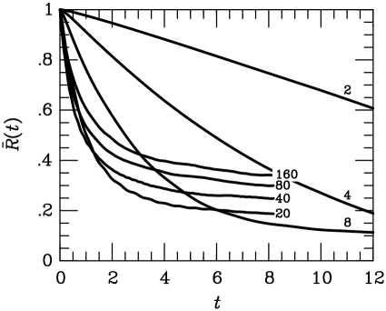
FIG. 5.: Correlation function $\bar{R}(t)$ for some of the runs of the Potential Strength series. The curves are marked with $V_{0}$.

FIG. 6.: Short-time behavior of $\bar{R}(t)$ for the runs P20 and P80 of the Potential Strength series.

In Fig. 5 we show $\bar{R}(t)$ for most of the runs; the curve for P16 falls almost exactly on top of P20. The runs P16–P160 show essentially the same relaxation behavior, except that the long-time value $\bar{R}_{\infty}$ increases with increasing potential strength. This is understood because for large potentials there are fewer low-lying energy levels that can be occupied by thermal nucleons, decreasing the effective number of energy eigenstates and thus increasing the importance of the diagonal term in the double sum of Eq. (24).

In order to quantify the overall relaxation behavior of the $\bar{R}(t)$ curves we approximate them by the ansatz

$$\bar{R}(t)=\bar{R}_{\infty}+(1-\bar{R}_{\infty})\,e^{-\Gamma_{1}t}.$$ (37)

The best-fit parameters are given in Table V. For the runs P2 and P4 a global fit was not meaningful because the overall integration time was too short.

The overall relaxation rate saturates and the saturation value is crudely estimated by $\Gamma_{\rm coll}$. Still, with increasing potential the short-time behavior changes significantly for the large potentials as illustrated in Fig. 6, i.e. an increasing $V_{0}$ still implies increasing power at higher modes of $\bar{S}(\omega)$. However, $\bar{R}(t)$ falls off more slowly than a global exponential because of its vanishing derivative at $t=0$. Hence the neutrino-cross section reduction is smaller than expected from the relaxation rate $\Gamma_{1}$, and saturates at larger values for $V_{0}$. The entries in Table V for $\Gamma_{\rm eff}$ confirm this trend; the saturation value for $\Gamma_{\rm eff}$ is very similar to that of $\Gamma_{1}$, i.e. about 1 MeV, but the potential strength at which this value is reached is $V_{0}\simeq 16$ for $\Gamma_{1}$, as compared to $V_{0}\simeq 80$ for $\Gamma_{\rm eff}$.

We may also compare $\Gamma_{\rm eff}$ with the simple Born estimate. Evidently, the Born approximation gives us a reasonable estimate of $\Gamma_{\rm eff}$ and thus of the cross-section suppression up to $V_{0}\lesssim 20$, but substantially overestimates $\Gamma_{\rm eff}$ for higher potential strengths.

Finally, we show in Fig. 7 the dynamical structure function $\bar{S}(\omega)$ obtained from cosine-transforming $\bar{R}(t)$. We actually show $\omega^{2}\bar{S}(\omega)$, a quantity that would asymptotically reach $2\Gamma$ for large $\omega$ if $\bar{S}(\omega)$ were a Lorentzian. For $V_{0}\gtrsim 12$ the power spectra develop a conspicuous resonance feature.

FIG. 7.: Dynamical structure function for the runs of the Potential Strength series.

Such resonance effects are even more important if we use a potential without a spin-independent repulsive term. This is illustrated by a similar series of runs with common characteristics summarized in Table VII and run-specific information in Table VII. Of course, in the perturbative regime a spin-independent potential has no effect on the spin relaxation rate so that the presence or absence of this term begins to show up only when the impact of the potentials is no longer small. The impact of the repulsive core on $\bar{R}(t)$ is illustrated by Fig. 8 for $V_{0}=20$ and $160$. The difference in $\Gamma_{\rm eff}$ is still $\simeq 10\%$ at $V_{0}=5$.

TABLE VI.: Parameters for series Resonances.

$b$	RC	$T$	$a$	$\rho_{s}$	$\Gamma_{\rm coll}$
1	no	30	1	0.1	2.81

TABLE VII.: Results for series Resonances.

Runa	$t_{\rm max}$	$10^{3}dt$	$n_{\rm s}$	$n_{\rm c}$	$\Gamma_{\rm Born}$	$\Gamma_{\rm eff}$
R5	65.536	2	20	23	0.0230	0.023
R10	32.768	2	20	54	0.0920	0.091
R20	16.384	2	20	92	0.368	0.37
R30	16.384	2	10	240	0.828	0.83
R40	8.192	1	5	932	1.47	1.51
R60	8.192	0.5	5	265	3.31	3.5
R80	4.096	0.25	5	280	5.89	6.3
R120	4.096	0.25	5	301	13.2	14.8
R160	2.048	0.125	5	213	23.5	28.5

^aRun R$n$ has a potential strength $V_{0}=n$.

FIG. 8.: Correlation functions with (dotted) and without (solid) a repulsive spin-independent core for the potential.

In Fig. 9 we show the dynamical structure function for some of these runs. When bound states are important, they have far more power at large frequencies than the previous runs with a repulsive core. Likewise, the effective relaxation rate $\Gamma_{\rm eff}$ increases with increasing $V_{0}$; there is no saturation. Indeed, both $\Gamma_{\rm Born}$ and $\Gamma_{\rm eff}$ scale as $V_{0}^{2}$. For all runs $\Gamma_{\rm Born}/\Gamma_{\rm eff}\approx 1$, and thus the Born approximation is surprisingly good, despite being not expected to be applicable according to Eq. (29). For $V_{0}=160$ we reach $\Gamma_{\rm eff}/T=1$, but of course, such large potentials are far beyond what appears plausible for a supernova core where bound-state effects probably do not dominate.

FIG. 9.: Dynamical structure function for some of the runs of the Resonance series.

E Variation of the Potential Width

In order to check to which degree the saturation value of $\Gamma_{\rm eff}$ for large potential strengths $V_{0}$ depends on the width $b$ of the potential, we have calculated $\Gamma_{\rm eff}$ for a series of combination of $V_{0}$ and $b$. For these runs the integration time was taken very short, just long enough to determine $\Gamma_{\rm eff}$, but not long enough to calculate a detailed power-spectrum or other global information. The common parameters for this series Potential Width are given in Table IX while the $\Gamma_{\rm eff}$-values are shown in Table IX.

TABLE VIII.: Parameters for series Potential Width.

RC	$T$	$a$	$\rho_{\rm s}$	$n_{s}$	$L$	$dt$	$t_{\rm max}$	$n_{c}$	$\Gamma_{\rm coll}$
yes	30	0.5	0.1	5	50	0.001	0.1	500	2.81

TABLE IX.: $\Gamma_{\rm eff}$ for series Potential Width.

	$V_{0}$
	25	50	75	100	125	150	175	200
$b=0.5$	0.13	0.33	0.47	0.55	0.57	0.58	0.54	0.52
1.0	0.31	0.73	0.96	1.08	1.07	1.03	0.95	0.93
1.5	0.50	1.12	1.48	1.63	1.59	1.54	1.46	1.39
2.0	0.68	1.53	2.03	2.19	2.12	2.11	1.98	1.90

The saturation value of $\Gamma_{\rm eff}$ increases with $b$, but for widths which represent the range of the nuclear force, it never reaches the “collision limit” $\Gamma_{\rm coll}$.

F Variation of the Density of Scatterers

As a next test we have varied the density of scatterers, keeping the potential strength fixed at $V_{0}=20$ where the efficiency of spin flips saturates according to the results of the previous section. We have performed two series of runs, one (D) where the potentials include a repulsive core to avoid bound states, and one (E) without this term. The common parameters for both series are given in Table XIII, while parameters and results specific to the series D and E are given in Tables XIII and XIII, respectively, and the dynamical spin structure functions for some of these cases are shown in Figs. 10 and 11. The runs are named D$n$ or E$n$ where $n$ is the number of scatterers in a given configuration.

TABLE X.: Parameters for series Density.

$V_{0}$	$b$	$T$	$a$	$L$	$t_{\rm max}$	$dt$
20	1	30	0.5	50	4.096	0.001

TABLE XI.: Results for Density (repulsive core).

Run	$\rho_{\rm s}$	$n_{\rm c}$	$\Gamma_{\rm coll}$	$\Gamma_{\rm Born}$	$\Gamma_{\rm eff}$
D10	0.2	166	5.6	0.736	0.46
D20	0.4	164	11.2	1.47	0.90
D40	0.8	164	22.5	2.94	1.76
D60	1.2	164	33.7	4.72	2.53
D100	2.0	146	56.2	7.36	4.1
D200	4.0	145	112	14.7	8.1
D600	12.0	340	337	44.2	27.9

TABLE XII.: Results for Density (no repulsive core).

Run	$\rho_{\rm s}$	$n_{\rm c}$	$\Gamma_{\rm coll}$	$\Gamma_{\rm Born}$	$\Gamma_{\rm eff}$
E1a	0.02	56	0.56	0.0736	0.067
E3b	0.06	60	1.69	0.221	0.234
E5b	0.10	54	2.81	0.368	0.38
E7b	0.14	60	3.93	0.515	0.51
E10	0.2	166	5.6	0.736	0.72
E20	0.4	166	11.2	1.47	1.39
E40	0.8	166	22.5	2.94	2.69
E60	1.2	166	33.7	4.42	4.0
E100	2.0	154	56.2	7.36	6.4
E200	4.0	163	112	14.7	11.6
E600	12.0	250	337	44.2	40.0

^a$t_{\rm max}=4\times 4.096$ and $dt=0.002$.
^b$t_{\rm max}=2\times 4.096$.

TABLE XIII.: Results for Density (repulsive core, $V_{0}=80$).

Run	$\rho_{\rm s}$	$n_{\rm c}$	$\Gamma_{\rm coll}$	$\Gamma_{\rm Born}$	$\Gamma_{\rm eff}$
DV3a	0.06	55	1.69	3.53	0.609
DV10b	0.2	40	5.6	11.8	1.95
DV40c	0.8	47	22.5	47.1	7.89
DV200c	4.0	425	112	235	54.3
DV600c	12.0	108	337	706	104

^a$t_{\rm max}=2\times 4.096$.
^b$dt=0.0005$.
^c$t_{\rm max}=4.096/2$ and $dt=0.0005$.

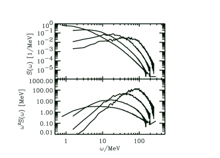
FIG. 10.: $\bar{S}(\omega)$ (upper panel) and $\omega^{2}\bar{S}(\omega)$ (lower panel) for some of the runs of the Density series with repulsive core. In decreasing order at the left end, the lines represent the runs D10, D40, D200, and D600.

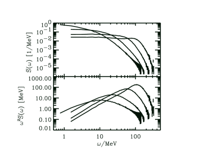
FIG. 11.: Same as Fig. 10, but for the Density series without repulsive core., i.e., the runs E10, E40, E200, and E600.

FIG. 12.: Effective relaxation rate for Density runs.

The effective relaxation rate grows linearly with density (Fig. 12) even for densities so large that the potentials significantly overlap with each other. We have observed that this holds for any potential strength as long as most of the energy eigenfunctions are not localized. The absence of saturation can also be seen from the dynamical structure functions themselves, Figs. 10 and 11. Note that at high densities the structure functions exhibit the flat behavior at low frequencies expected from the classical picture, Eq. (9), in the case without a repulsive core, whereas in the presence of a repulsive core they increase with frequency.

As soon as the potentials are strong enough and/or the density is high enough for a significant fraction of the energy eigenfunctions to become localized we observe a saturation in $\rho_{s}$, as demonstrated in Table XIII which lists results for potentials of strength $V_{0}=80$ and with a repulsive core. This can be understood qualitatively by observing that $\left|\left\langle n|\hat{\hbox{\boldmath$\sigma$}}(0,{\bf k})|n\right\rangle\right|^{2}$ is independent of the box size $L$ for a localized eigenstate $|n\rangle$, as opposed to decreasing with $L$ for a non-localized state, and thus gives rise to an asymptotic non-vanishing $\bar{R}_{\infty}$ in the continuum limit $L\to\infty$, preventing the scattering cross section $\langle\sigma\rangle$ to decrease further [see Eq. (B9)]. At the same time, we expect the test-particle approximation adopted in the present work to break down in the regime with a significant fraction of localized states.

Outside this regime, the highest effective spin fluctuation rate and the strongest scattering cross section suppression we found were $\Gamma_{\rm eff}/T\simeq 2$ and $\langle\sigma\rangle/\sigma_{0}\simeq 0.5$ for $V_{0}\simeq 80$, $\rho_{s}\simeq 4$, about a factor 2 smaller than $\Gamma_{\rm coll}$, see Table XIII.

Finally, to get a better overview of the saturation behavior for large potential strengths $V_{0}$ in the presence of a repulsive core, we have calculated $\Gamma_{\rm eff}$ for a series of combination of $V_{0}$ and $\rho_{s}$. Again, for these runs the integration time was taken very short. The common parameters for this series Strength-Density are given in Table XV while the $\Gamma_{\rm eff}$-values are shown in Table XV.

TABLE XIV.: Parameters for series Strength-Density.

$b$	RC	$T$	$a$	$L$	$dt$	$t_{\rm max}$	$n_{c}$
1	yes	30	1	50	0.001	0.1	500

TABLE XV.: $\Gamma_{\rm eff}$ for series Strength-Density.

		$V_{0}$
		25	50	75	100	150
$\rho_{s}=0.1$	$\Gamma_{\rm coll}=2.81$	0.32	0.70	0.92	1.03	0.99
0.5	14.0	1.59	3.6	4.7	5.4	5.2
1.0	28.1	3.1	7.1	9.7	10.9	11.4
2.0	56.2	6.2	14.5	22.	27.	38.
4.0	112.4	12.8	33.	50.	64.	87.

Again, even for extreme combinations of density and potential strength, does $\Gamma_{\rm eff}$ stay safely below the collisional estimate $\Gamma_{\rm coll}$. For combinations which may plausibly mimic nuclear matter, $\Gamma_{\rm eff}$ always stays below $T$.

V Discussion and Summary

We have numerically studied the relaxation behavior of a single nucleon which moves in a one-dimensional box, filled with a certain density of spin-dependent scatterers. This simple model is meant to mimic the collisional broadening of the dynamical nucleon spin-density structure function in a supernova core.

In most runs, the potential was modelled as a Gaussian with a width of $1~{}{\rm fm}$ as suggested by the range of the one-pion exchange force which is the primary cause for nucleon spin fluctuations. However, the exact range of the potential has no significant impact on our conclusion.

In order to quantify the spin relaxation behavior by a single number we have chosen an effective spin relaxation rate $\Gamma_{\rm eff}$ which is defined as the width of a Lorentzian structure function which produces the same neutrino-nucleon cross section suppression. For sufficiently weak potentials, our numerical runs reproduce the perturbative value in Born-approximation.

When the potential has a repulsive core such that bound states cannot form, the spin-relaxation rate saturates with increasing potential strength at a value which is a factor 2–3 smaller than one would have expected from a classical analogy where one pictures the spin as being randomized each time the nucleon encounters a scattering center. The saturation value for the potential strength roughly coincides with the value when the Born approximation begins to break down, and where bound states begin to form in the absence of the repulsive core. For the range $1~{}{\rm fm}$ of our Gaussian potential this is at a potential strength of around 20 MeV which also is typical for the spin-interaction energy between two nucleons.

Furthermore, we observed that the spin-relaxation rate is roughly linear in the density of scatterers. This is expected in the classical picture, but our simulations show that it even holds if the potentials overlap substantially. Saturation is only observed for densities high and/or potentials strong enough for the formation of a substantial fraction of localized energy eigenstates. However, in this regime, a strong correlation of neighboring nucleon spins is expected, and the test-particle approximation adopted in our work is no longer meaningful.

When the scattering potentials lead to bound states (no repulsive core), there is no saturation of $\Gamma_{\rm eff}$, not with increasing potential strength and not with an increasing density of scatterers. Instead, the spin-relaxation rate follows the Born approximation amazingly closely, despite the fact that it is not applicable. However, the test-particle approximation again is not viable as a model for a nuclear medium because the bound states which dominate in this regime signal the importance of spin-spin-correlations.

In any case, we expect the case of repulsive potentials without strongly bound states to be more appropriate as a model for the conditions in a supernova core because of the relevant properties of nuclear matter. In this situation, the value $\Gamma_{\rm coll}$ derived from a classical picture provides an upper limit for the spin-fluctuation rate which saturates for potential strengths expected from nuclear interactions within about a factor 2, and captures the linear dependence on the one-dimensional density in the regime where spatial spin correlations are small and the test-particle approximation is applicable.

For combinations of density and potential strength which do not look like absurd overestimates of what is appropriate for nuclear matter, the spin-fluctuation rate is always safely below the temperature, and the scattering cross-section suppression is at most a few ten percent. The Born approximation, in contrast, significantly overestimates the spin-fluctuation rate and predicts far too large cross-section reductions.

Naturally, the conclusions from our one-dimensional model do not directly carry over to three dimensions, but can only be taken as an indication of what one might expect. If the classical collision rate for three dimensions embodied by our Eq. (10) is taken as an upper limit for the spin relaxation rate, then again a naive Born-approximation calculation is a significant overestimate, and the true collisional broadening of $S(\omega,k)$ is too small to cause a significant cross-section reduction.

Our calculations also indicate that the Born approximation, while being a significant overestimate of the spin-relaxation rate, it is not an absurd overestimate. For the relevant conditions it may overestimate $\Gamma$ by a factor of a few, but not by orders of magnitude. Therefore, we do not expect that quantities like the axion or neutrino-pair emission rate, which depend on the collisional broadening of $S(\omega,k)$, suffer much of an additional suppression beyond those discussed in Ref. [5].

From our simple toy model we find no evidence for extreme deviations from the overall picture developed in Ref. [5, 10], which may be summarized by saying that spin fluctuations look small enough to avoid excessive neutrino opacity reductions, but large enough to avoid huge reductions of the axion or neutrino pair emissivities.

Clearly, more accurate and detailed calculations should be performed in three dimensions with realistic nucleon interaction potentials. Furthermore, a treatment of the high-density limit should go beyond the test-particle approximation and apply a full quantum Monte Carlo approach [12] to finite temperature and nuclear matter.

A Perturbative Estimate of $\Gamma$

From a perturbative calculation of the bremsstrahlung process $NN\to NN\nu\bar{\nu}$ one can easily extract the (unresummed) dynamical structure function. For nondegenerate nucleons and on the basis of a one-pion exchange potential it has been evaluated in Ref. [4]; even for the conditions of a supernova core this potential should be a reasonable representation of the tensor force [8]. The result was written in the form

$$\bar{S}^{(1)}(\omega)=\frac{\Gamma_{\sigma}}{\omega^{2}}\,\bar{s}(\omega/T),$$ (A1)

where $\bar{s}(x)$ is a slowly varying dimensionless function of order 1, normalized such that $\bar{s}(0)=1$. Further, $\Gamma_{\sigma}=4\sqrt{\pi}\,\alpha_{\pi}^{2}\,n_{N}T^{1/2}m_{N}^{-5/2}$ with $n_{N}$ the nucleon density, $m_{N}$ the nucleon mass, and $\alpha_{\pi}\equiv(f2m/m_{\pi})^{2}/4\pi\approx 15$ with $f\approx 1$ the pion-nucleon “fine-structure constant.” The function $\bar{s}$ is explicitly

$$\bar{s}(x,y) = \frac{e^{-x/2}+e^{x/2}}{16}\int_{|x|}^{\infty}dt\,\,e^{-t/2}\,\,\frac{3x^{2}+6ty+5y^{2}}{3}$$ (A4)

$${}\times\Biggl{[}\frac{2\sqrt{t^{2}-x^{2}}}{x^{2}+2ty+y^{2}}$$

$$\hskip 20.00003pt{}-\frac{1}{t+y}\,\log\left(\frac{t+y+\sqrt{t^{2}-x^{2}}}{t+y-\sqrt{t^{2}-x^{2}}}\right)\Biggr{]},$$

where $x=\omega/T$ and pion-mass effects are included by virtue of the parameter $y\equiv m_{\pi}^{2}/m_{N}T=19.4~{}{\rm MeV}/T$. We show $\bar{s}(x,y)$ in Fig. 13 for several values of $y$.

FIG. 13.: Dimensionless structure function according to Eq. (A4) for $y=0,\ldots,2$ in steps of 0.5.

For temperatures between 10 and $40~{}{\rm MeV}$, corresponding to $y=0.5$–2, this function is approximately constant for a large range of $x=\omega/T$. If we approximate it by $1/2$ we may write $\bar{S}^{(1)}(\omega)\approx 2\Gamma/\omega^{2}$ with $\Gamma=\Gamma_{\sigma}/4$ or

$$\gamma\equiv\frac{\Gamma}{T}=\frac{\sqrt{\pi}\,\alpha_{\pi}^{2}\,n_{N}}{T^{1/2}m_{N}^{5/2}}=1.24\,\rho_{14}\,T_{30}^{-1/2},$$ (A5)

where $\rho_{14}=\rho/10^{14}~{}{\rm g}~{}{\rm cm}^{-3}$ and $T_{30}=T/30~{}{\rm MeV}$. Even if $\gamma$ is only a few is enough to imply a significant cross-section suppression (Appendix B).

B Cross-Section Reduction

The reduction of the axial-current neutrino-nucleon scattering cross section $\sigma$ by spin fluctuations was discussed in detail in Ref. [7]. With $\sigma_{0}$ the vacuum cross section and $\langle\cdots\rangle$ an average over a Maxwell-Boltzmann distribution of neutrino energies, one finds [7]

$$\frac{\langle\sigma\rangle}{\langle\sigma_{0}\rangle}=\int_{0}^{\infty}\frac{d\omega}{2\pi}\,S(\omega)\,\left[2+\frac{\omega}{T}+\frac{1}{6}\,\left(\frac{\omega}{T}\right)^{2}\right]\,e^{-\omega/T}.$$ (B1)

Equivalently, the amount of reduction can be expressed in the form

$$\frac{\delta\langle\sigma\rangle}{\langle\sigma_{0}\rangle}=-\int_{0}^{\infty}\frac{d\omega}{2\pi}\,S(\omega)\,G(\omega/T),$$ (B2)

where the dimensionless phase-space weight function is

$$G(x)=1-(1+x+x^{2}/6)\,e^{-x}.$$ (B3)

This representation is needed to determine the suppression when the structure function $S(\omega)$ is given by an un-resummed perturbative expression and thus diverges at $\omega=0$.

We show the cross-section suppression Eq. (B1) in Fig. 14 as a function of $\gamma=\Gamma/T$ for our generic structure function

$$S(\omega)=\frac{2\Gamma}{\omega^{2}+\Gamma^{2}}\,\frac{2}{1+e^{-\omega/T}}$$ (B4)

implied by Eqs. (7) and (9). Limiting cases are

$$\frac{\langle\sigma\rangle}{\langle\sigma_{0}\rangle}=\cases{1-A\gamma&for $\gamma\ll 1$,\cr B/\gamma&for $\gamma\gg 1$.\cr}$$ (B5)

The coefficients are

$$A = \frac{2}{\pi}\int_{0}^{\infty}dx\,\frac{e^{x}-(1+x+x^{2}/6)}{x^{2}(1+e^{x})}=0.438703,$$ (B6)

$$B = \frac{2}{\pi}\int_{0}^{\infty}dx\,\frac{2+x+x^{2}/6}{1+e^{x}}=1.59745.$$ (B7)

We will need to know the value of $\gamma$ corresponding to a given cross-section suppression $s=|\delta\langle\sigma\rangle/\langle\sigma_{0}\rangle|$. An approximation formula, good to within about 1%, is

$$\gamma(s)=\frac{B\,(1-\sqrt{1-s})\,s}{1-s}+\frac{s}{A\sqrt{1-s}}.$$ (B8)

It is essentially an interpolation between the inversions of the limiting functions of Eq. (B5).

FIG. 14.: Suppression of the average axial-current neutrino-nucleon scattering cross section according to Eq. (B1).

In our present study, the primary quantity produced by the numerical runs is $\bar{R}(t)$. Therefore, we finally express Eq. (B1) in its Fourier transformed version,

$$\frac{\langle\sigma\rangle}{\langle\sigma_{0}\rangle}=\int_{0}^{\infty}d\tau\,\bar{R}(\tau/T)\,F(\tau)$$ (B9)

where

$$F(\tau)=\frac{2}{\pi}\int_{0}^{\infty}dx\,\cos(x\tau)\,\frac{2+x+x^{2}/6}{1+e^{x}},$$ (B10)

shown in Fig. 15. It is normalized as $\int_{0}^{\infty}d\tau\,F(\tau)=1$ and $F(0)=B=[\pi^{2}+12\log(4)+3\zeta(3)]/6\pi=1.59745$.

FIG. 15.: Function $F(\tau)$ according to Eq. (B10).

REFERENCES

- [1] R.F. Sawyer, Phys. Rev. C 40, 865 (1989).
- [2] A. Burrows and R. Sawyer, Phys. Rev. C 58, 554 (1998). A. Burrows and R. Sawyer, submitted to Phys. Rev. Lett., astro-ph/9804264.
- [3] S. Reddy and M. Prakash, Astrophys. J. 478, 689 (1997). S. Reddy, M. Prakash and J.M. Lattimer, Phys. Rev. D 58, 013009 (1998).
- [4] G. Raffelt and D. Seckel, Phys. Rev. D 52, 1780 (1995).
- [5] H.-T. Janka, W. Keil, G. Raffelt and D. Seckel, Phys. Rev. Lett. 76, 2621 (1996).
- [6] R.F. Sawyer, Phys. Rev. Lett. 75, 2260 (1995).
- [7] G. Raffelt, D. Seckel and G. Sigl, Phys. Rev. D 54, 2784 (1996).
- [8] S. Hannestad and G. Raffelt, to be published in Astrophys. J., astro-ph/9711132.
- [9] W. Keil, H.-T. Janka, and G. Raffelt, Phys. Rev. D 51, 6635 (1995).
- [10] G. Sigl, Phys. Rev. Lett. 76, 2625 (1996).
- [11] G. Sigl, Phys. Rev. D 56, 3179 (1997).
- [12] S. E. Koonin, D. J. Dean, and K. Langanke, Phys. Rep. 278, 1 (1997).