hep-ph/9808469

Domain Walls and Theta Dependence in QCD

with an Effective Lagrangian Approach
Todd Fugleberg , Igor Halperin and Ariel Zhitnitsky
Physics and Astronomy Department

University of British Columbia

6224 Agricultural Road, Vancouver, BC V6T 1Z1, Canada

e-mail: fugle@physics.ubc.ca
higor@physics.ubc.ca
arz@physics.ubc.ca

PACS numbers: 12.38.Aw, 11.15.Tk, 11.30.-j.
Abstract:

We suggest an anomalous effective Lagrangian which reproduces the anomalous conformal and chiral Ward identities and topological charge quantization in QCD. It is shown that the large $N_{c}$ Di Vecchia-Veneziano-Witten effective chiral Lagrangian is locally recovered from our results, along with $1/N_{c}$ corrections, after integrating out the heavy “glueball” fields. All dimensionful parameters in our scheme are fixed in terms of the quark and gluon condensates and quark masses. We argue that for a certain range of parameters, metastable vacua appear which are separated from the true vacuum of lowest energy by domain walls. The surface tension of the wall is estimated, and the dynamics of the wall is discussed. The U(1) problem and the physics of the pseudo-goldstone bosons at different $\theta$ angles are addressed within the effective Lagrangian approach. Implications for axion physics, heavy ion collisions and the development of the early Universe during the QCD epoch are discussed.

1 Introduction

The effective Lagrangian techniques have proved to be a powerful tool in quantum field theory. Generally, there exist two different definitions of an effective Lagrangian. One of them is the Wilsonian effective Lagrangian describing the low energy dynamics of the lightest particles in the theory. In QCD, this is implemented by effective chiral Lagrangians (ECL’s) for the pseudoscalar mesons, which are essentially constrained by the global non-anomalous $SU(N_{f})\times SU(N_{f})$ and (for large $N_{c}$) anomalous $U(1)$ chiral symmetries. Another type of effective Lagrangian (action) is defined as the Legendre transform of the generating functional for connected Green functions. This object is relevant for addressing the vacuum properties of the theory in terms of vacuum expectation values (VEV’s) of composite operators, as they should minimize the effective action. Such an approach is suitable for the study of the dependence of the QCD vacuum on external parameters, such as the light quark masses or the vacuum angle $\theta$. The lowest dimensional condensates $\langle\bar{\Psi}\Psi\rangle,\langle G^{2}\rangle,\langle G\tilde{G}\rangle$, which are the most essential for the QCD vacuum structure, are related to the anomalously and explicitly broken conformal and chiral symmetries of QCD. Thus, one can study the vacuum of QCD with an effective Lagrangian realizing at the tree level anomalous conformal and chiral Ward identities of the theory. The utility of such an approach to gauge theories has been recognized long ago for supersymmetric (SUSY) models, where anomalous effective Lagrangians were found for both the pure gauge case [1] and super-QCD (SQCD) [2].

The purpose of this paper is a detailed analysis of the anomalous effective Lagrangian for QCD with $N_{f}$ light flavors and $N_{c}$ colors (more precisely, of its potential part) which was suggested recently by two of us, and briefly described in [3]. It was obtained as a generalization of an anomalous effective Lagrangian for pure YM theory which was proposed earlier in [4]. The constructions of [4] and [3] can be viewed as non-supersymmetric counterparts of the Veneziano-Yankielowicz (VY) effective potential [1] for SUSY YM theory and the Taylor-Veneziano-Yankielowicz (TVY) effective potential for SQCD, respectively. The results obtained in [4, 3] reveal some striking similarities between the supersymmetric and non-supersymmetric effective potentials and the physics that follows. Notably, the effective potentials for QCD and gluodynamics are holomorphic functions of their fields, analogously to the SUSY case. Moreover, they have both “dynamical” and “topological” parts - a structure which is similar to that of the (amended [5]) VY effective potential [1]. As will be discussed in detail below, this “topological” part of the effective potential turns out to be crucial for the analysis of the physical $\theta$ dependence in QCD.

The interest in such an effective Lagrangian for anomalously broken conformal and chiral $U(1)$ symmetries is several-fold. First, it provides a generalization of the large $N_{c}$ Di Vecchia-Veneziano-Witten (VVW) ECL [6] (see also [7]) for the case of arbitrary $N_{c}$ after integrating out the massive “glueball” fields. At this stage, no holomorphy is present in the resulting effective chiral potential. In this way we arrive at a Wilsonian effective Lagrangian for the light degrees of freedom consistent with the Ward identities of the theory and a built-in quantization of the topological charge (see below). One may note that in principle such a Wilsonian effective Lagrangian satisfying all general requirements on the theory could also be written down without constructing first a more complicated anomalous effective potential including also the “glueball” degrees of freedom. The resulting effective potential is found to contain a sine-Gordon term whose large $N_{c}$ expansion reproduces the VWW effective potential in the vicinity of the global minimum, along with $1/N_{c}$ corrections. The presence of such term in the effective potential implies that the theory sustains the domain wall excitations. This observation may be important in the contexts of cosmology and heavy ion collisions. Furthermore, our two-step approach to the derivation of the effective chiral Lagrangian has an additional merit in that all dimensionful parameters in our scheme are fixed in terms of the gluon and quark condensates and quark masses. (The only entries which are not fixed in our scheme are two dimensionless integer-valued parameters related to the vacuum structure and $\theta$ dependence of the theory. As their values are still a subject of some controversy, see Sect. 3, in most of the paper we will keep them as free parameters.) The absence of free dimensionful parameters helps to better understand the origin of the $\eta^{\prime}$ mass (the famous U(1) problem). In particular, it yields a new mass formula for the $\eta^{\prime}$ for finite $N_{c}$ in terms of quark and gluon condensates in QCD (see Eq.(59) below). Second, it allows one to address related questions of the phenomenology of pseudoscalar mesons, such as $\pi^{0}-\eta-\eta^{\prime}$ or $\eta-\eta^{\prime}$ mixing with no further phenomenological input. Third, such an effective Lagrangian allows one to address the problem of $\theta$ dependence in QCD. In contrast to the approach of Ref.[6] which deals from the very beginning with the light chiral degrees of freedom and explicitly incorporates the $U_{A}(1)$ anomaly without restriction of the topological charge to integer values, in our method both the $U_{A}(1)$ anomaly and topological charge quantization are included in the effective Lagrangian framework. After the “glueball” fields are integrated out, the topological charge quantization still shows up in the limit $V\rightarrow\infty$ via the presence of certain cusps in the effective potential, which are not present in the large $N_{c}$ ECL of Ref.[6]. Analogous “glued” effective potentials containing cusp singularities arise in supersymmetric $N=1$ theories when quantization of the topological charge is imposed [5, 8, 9]. As will be discussed below, these modifications are not essential for the local properties of the effective chiral potential in the vicinity of the global minimum. In this case, the results of Ref.[6] are reproduced along with calculable $1/N_{c}$ corrections. On the other hand, for large values of $\theta$ and/or $\phi_{i}$ our results deviate from those of [6]. Last but not least, the problem of the $\theta$ dependence in QCD is directly relevant for the construction of a realistic axion potential that would be compatible with the Ward identities of QCD. This is because an axion potential $V(a)$ can be obtained, provided the functional form of the vacuum energy in QCD $E_{vac}(\theta)$ is known, by the formal substitution $\theta\rightarrow a(x)/f_{a}$.

Our presentation is organized as follows. In Sect. 2 we describe the approach of Refs. [4] and [3] to the construction of an anomalous effective Lagrangian for pure YM theory and QCD, respectively. Sect. 3 discusses different proposals to find the dimensionless integer-valued parameters that enter our results. A particular method suggested in [10] to fix these numbers in the context of pure YM theory is presented in an appendix in a form adopted for the case of full QCD. In Sect. 4 we show how the heavy “glueball” degrees of freedom in our effective potential can be integrated out, thus yielding an effective chiral potential for the light degrees of freedom. A correspondence with the VWW ECL [6] is established. In Sect. 5 we discuss the vacuum properties, $\theta$ dependence and domain wall solutions in the resulting effective theory. Sect. 6 is devoted to an analysis of the U(1) problem and properties of the pseudo-goldstone bosons at zero and non-zero $\theta$. Sect. 7 deals with the implications of our results for the properties of the axion and a possible study of the $\theta$ dependence and new axion search experiment at RHIC. We also discuss the possibility of baryogenesis at the QCD scale, which seems suggestive in view of our results.

2 Anomalous effective Lagrangian for QCD

We start with recalling the construction [4] of the anomalous effective potential for pure YM theory (gluodynamics). It is defined as the Legendre transform of the generating functional for zero momentum correlation functions of the marginal operators $G_{\mu\nu}\tilde{G}_{\mu\nu}$ and $G_{\mu\nu}G_{\mu\nu}$ which are fixed by the conformal anomaly in terms of the gluon condensate [11, 12]. The effective potential is a function of effective zero momentum fields $h,\bar{h}$ which describe the VEV’s of the composite complex fields $H,\bar{H}$ :

$$\int dx\,h=\langle\int dx\,H\rangle\;\;,\;\;\int dx\,\bar{h}=\langle\int dx\,\bar{H}\rangle\;,$$ (1)

where

$$H=\frac{1}{2}\left(\frac{\beta(\alpha_{s})}{4\alpha_{s}}G^{2}+i\,\frac{1}{\xi_{YM}}\frac{\alpha_{s}}{4\pi}G\tilde{G}\right)\;,\;\bar{H}=\frac{1}{2}\left(\frac{\beta(\alpha_{s})}{4\alpha_{s}}G^{2}-i\,\frac{1}{\xi_{YM}}\frac{\alpha_{s}}{4\pi}G\tilde{G}\right)\;.$$ (2)

and $\beta(\alpha_{s})=-b_{YM}\alpha_{s}^{2}/(2\pi)+O(\alpha_{s}^{3})$ , $b_{YM}=(11/3)N_{c}$ is the Gell-Mann - Low $\beta$-function for YM theory , and $\xi_{YM}$ is a generally unknown parameter which parametrizes the correlation function of the topological density

$$\lim_{q\rightarrow 0}\;i\int dx\,e^{iqx}\langle 0|T\left\{\frac{\alpha_{s}}{8\pi}G\tilde{G}(x)\,\frac{\alpha_{s}}{8\pi}G\tilde{G}(0)\right\}|0\rangle_{YM}=\xi_{YM}^{2}\,\langle\frac{\beta(\alpha_{s})}{4\alpha_{s}}G^{2}\rangle_{YM}\;.$$ (3)

The two-point function (3) and other zero momentum correlation functions of $\alpha_{s}G^{2},\alpha_{s}G\tilde{G}$ are defined via the Wick type T-product by the nonperturbative part of the partition function $\log(Z(\theta)/Z_{PT})$ ( $Z_{PT}$ stands for a perturbatively defined partition function which does not depend on $\theta$), where

$$Z(\theta)=Z_{PT}\exp\left\{-iVE_{v}(\theta)\right\}=Z_{PT}\,\exp\left\{-iV\langle 0|\frac{\beta(\alpha_{s})}{16\alpha_{s}}G^{2}|0\rangle_{\theta}\right\}\;$$ (4)

by differentiation with respect to the bare coupling constant $1/g_{0}^{2}$ and $\theta$. In Eq.(4) we used the fact that the vacuum energy is defined relatively to its value in perturbation theory by a nonperturbative part of the conformal anomaly, for any $\theta$. When the vacuum expectation value (VEV) in Eq.(4) is defined in this way, its dependence on $1/g_{0}^{2}$ is fixed by the dimensional transmutation formula

$$\langle-\frac{b\alpha_{s}}{8\pi}G^{2}\rangle=const\,\left[M_{R}\exp\left(-\frac{8\pi^{2}}{bg_{0}^{2}}\right)\right]^{4}\;.$$ (5)

Here $M_{R}$ is the ultraviolet cut-off mass, and the one-loop $\beta$-function is used. It is important to stress that different regularization schemes generally lead to different values of the constant in Eq.(5) but, once specified, the VEV (5) determines all zero momentum correlation functions of $\beta(\alpha_{s})/(4\alpha_{s})G^{2}$, with perturbative tails subtracted. At $\theta=0$, Eq.(3) follows from Eq.(4) using the general relation [4]

$$\langle\frac{\beta(\alpha_{s})}{4\alpha_{s}}G^{2}\rangle_{\theta}=\langle\frac{\beta(\alpha_{s})}{4\alpha_{s}}G^{2}\rangle_{0}\;f(\theta)\;\;,\;\;f(\theta)\equiv 1-2\xi^{2}\,\theta^{2}+O(\theta^{4})\;.$$ (6)

The strong assumption made in [4] was that Eq.(3) is actually covariant in $\theta$, i.e. remains valid for any (at least, small) value of $\theta$. The assumption of covariance in $\theta$ is reproduced a posteriori from the effective Lagrangian, and is thus self-consistent. We note that covariance of Eq.(3) in $\theta$ follows automatically within the approach suggested in [12]. In fact, it is this conjectured covariance of Eq.(3) in $\theta$ that underlies the holomorphic structure of the resulting effective potential (see Eq.(9) below). Thus, we are not able at the moment to prove holomorphy, but instead argue that it is there based on (i) self-consistency of this proposal (see Sect.3), and (ii) the possibility of comparing our final formulas with the known results (such as the large $N_{c}$ effective chiral Lagrangian and anomalous Ward identities in QCD, see Sect.4), and the experience from the known models.

The advantage of using the combinations (2) is in the holomorphic structure of zero momentum correlation functions of operators $G^{2}\,,\,G\tilde{G}$ written in terms of the $H,\bar{H}$ fields [4, 10]:

$$\lim_{q\rightarrow 0}\,i\int dxe^{iqx}\langle 0|T\{H(x)\;H(0)\}|0\rangle = -4\langle H\rangle\;,$$

$$\lim_{q\rightarrow 0}\,i\int dxe^{iqx}\langle 0|T\{\bar{H}(x)\;\bar{H}(0)\}|0\rangle = -4\langle\bar{H}\rangle\;,$$ (7)

$$\lim_{q\rightarrow 0}\,i\int dxe^{iqx}\langle 0|T\{\bar{H}(x)\;H(0)\}|0\rangle = 0\;.$$

In what follows Eqs.(2) will be sometimes referred to as the anomalous Ward identities (WI’s). It can be seen that the n-point zero momentum correlation function of the operator $H$ equals $(-4)^{n-1}\langle H\rangle$. Multi-point correlation functions of the operator $\bar{H}$ are analogously expressed in terms of its vacuum expectation value $\langle\bar{H}\rangle$. At the same time, it is easy to check that the decoupling of the fields $H$ and $\bar{H}$ holds for arbitrary n-point functions of $H$, $\bar{H}$. This is the origin of holomorphy of an effective Lagrangian for YM theory, which codes information on all anomalous WI’s.

One should note that the right hand side of the last equation in (2) does contain perturbative contributions proportional to regular powers of $\alpha_{s}$. However, they are irrelevant for our purposes, as we are only interested in the decoupling of the fields $H$ and $\bar{H}$ at the level of nonperturbative $O(e^{-1/\alpha_{s}})$ effects. Holomorphy of an effective potential for YM theory has the same status. Thus, in contrast to the supersymmetric case where holomorphy is an exact property of the effective superpotential, in the present case it only refers to a “nonperturbative” effective potential which does not include perturbative effects to any finite order in $\alpha_{s}$. We assume that perturbative and nonperturbative effects can be separated, at least in principle or/and by some suitable convention [12, 4]. As a result, a perturbatively defined partition function $Z_{PT}$ bearing a non-holomorphic dependence on $g_{0}^{2}$ decouples in zero momentum correlation functions. On the other hand, the $\theta$ dependence appears only in the nonperturbative part of $Z_{\theta}$. Thus, the nonperturbative vacuum energy depends only on a single complex combination $\tau=1/g_{0}^{2}+i\theta bq/(32\pi^{2}p)$ [12, 10]. Indeed, arguments based on renormalizability, analogous to those used in Ref. [11] (see also Sect. 3), imply the relation

$$\langle-\frac{b\alpha_{s}}{8\pi}G^{2}\rangle_{\theta}=const\;Re\;M_{0}^{4}\exp\left(-\frac{32\pi^{2}}{bg_{0}^{2}}-i\frac{q}{p}\theta\right)\equiv const\;Re\;M_{0}^{4}\exp\left(-\frac{32\pi^{2}}{b}\tau\right)\;.$$ (8)

(This expression coincides with the result obtained in [4] directly from the effective Lagrangian (9).) This is exactly the origin of the relations (2) which are obtained by differentiation of $\log(Z_{\theta}/Z_{PT})$ with respect to the holomorphic sources $\tau,\bar{\tau}$. Thus, once an assumption of separation of perturbative and nonperturbative contributions in Eq. (4) is made, a new complex structure emerges due to the nonperturbative origin of the $\theta$ parameter which combines with another parameter $1/g_{0}^{2}$ into the unique complex combination $\tau$.

The final answer for the improved effective potential $W(h,\bar{h})$ (here ’improved’ refers to the necessity of summation over the integers $n,k$ in Eq.(9), see below) reads [4]

$$e^{-iVW(h,\bar{h})} = \sum_{n=-\infty}^{+\infty}\sum_{k=0}^{q-1}\exp\left\{-\frac{iV}{4}\left(h\,Log\,\frac{h}{C_{YM}}+\bar{h}\,Log\,\frac{\bar{h}}{\bar{C}_{YM}}\right)\right.$$ (9)

$$+ \left.i\pi V\left(k+\frac{q}{p}\,\frac{\theta+2\pi n}{2\pi}\right)\frac{h-\bar{h}}{2i}\right\}\;,$$

where the constants $C_{YM},\bar{C}_{YM}$ can be taken to be real and expressed in terms of the vacuum energy in YM theory at $\theta=0$, $C_{YM}=\bar{C}_{YM}=-2eE_{v}^{(YM)}(0)=-2e\langle-b_{YM}\alpha_{s}/(32\pi)G^{2}\rangle$, and $V$ is the 4-volume. The integer numbers $p$ and $q$ are relatively prime and related to the parameter $\xi$ introduced in Eq.(3) by $q/p=2\xi$. Thus, we expect that the parameter $\xi$ defined in Eqs.(2),(3) is a rational number. This expectation is motivated by the fact that it turns out to be the case in all existing proposals to fix the value of $\xi$, to be discussed in the next section, and by experience with supersymmetric models. (In all likelihood, irrational values of $\xi$ would produce a non-differentiable $\theta$ dependence for YM theory.) On general grounds, it follows that $p=O(N_{c})\,,\,q=O(N_{c}^{0})$. The symbol $Log$ in Eq.(9) stands for the principal branch of the logarithm. The effective potential (9) produces an infinite series of anomalous WI’s. By construction, it is a periodic function of the vacuum angle $\theta$ . The effective potential (9) is suitable for a study of the YM vacuum as described above.

The double sum over the integers $n,k$ in Eq.(9) appears as a resolution of an ambiguity of the effective potential as defined from the anomalous WI’s. As was discussed in [4], this ambiguity is due to the fact that any particular branch of the multi-valued function $h\log(h/c)^{p/q}$, corresponding to some fixed values of $n,k$, satisfies the anomalous WI’s. However, without the summation over the integers $n,k$ in Eq.(9), the effective potential would be multi-valued and unbounded from below. An analogous problem arises with the original VY effective Lagrangian. It was cured by Kovner and Shifman in [5] by a similar prescription of summation over all branches of the multi-valued VY superpotential. Moreover, the whole structure of Eq.(9) is rather similar to that of the (amended) VY effective potential. Namely, it contains both the “dynamical” and “topological” parts (the first and the second terms in the exponent, respectively). The “dynamical” part of the effective potential (9) is similar to the VY [1] potential $\sim S\log(S/\Lambda)^{N_{c}}$ (here $S$ is an anomaly superfield), while the “topological” part is akin to the improvement [5] of the VY effective potential. Similarly to the supersymmetric case, the infinite sum over $n$ reflects the summation over all integer topological charges in the original YM theory. The difference of our case from that of supersymmetric YM theory is that an effective potential of the form $(1/N)\phi\log(\phi/\Lambda)^{N}$ , as in the SUSY case, implies a simpler form of the “topological” term $\sim 2\pi in/N\,(\phi-\bar{\phi})$ with only one “topological number” $n$ which specifies the particular branch of the multi-valued logarithm. In our case, we allow for a more general situation when the parameter $N$ is a rational number $N=p/q$. In this case we have two integer valued “topological numbers” $n$ and $k$, specifying the branches of the logarithm and rational function, respectively. Our choice is related to the fact that some proposals to fix the values of $p,q$ suggest that $q\neq 1$, see Sect. 3. (As follows from Eq.(8), the values of $p,q$ are fixed if the $\theta$ dependence is known.) One may expect that the integers $p$ and $q$ are related to a discrete symmetry surviving the anomaly, which may not be directly visible in the original fundamental Lagrangian.

It should be stressed that the improved effective potential (9) contains more information in comparison to that present in the anomalous Ward identities just due to the presence of the “topological” part in Eq.(9). Without this term Eq.(9) would merely be a kinematical reformulation of the content of anomalous Ward identities for YM theory. The reason is that the latter refer, as usual, to the infinite volume (thermodynamic) limit of the theory, where only one state of a lowest energy (for $\theta$ fixed) survives. This state corresponds to one particular branch of the multi-valued effective potential in Eq.(9). At the same time, the very fact of multi-valuedness of the effective potential implies that there are other vacua which should all be taken into consideration when $\theta$ is varied. When summing over the integers $n\,,\,k$, we keep track of all (including excited) vacua of the theory, and simultaneously solve the problems of multi-valuedness and unboundedness from below of the “one-branch theory”. The most attractive feature of the proposed structure of the effective potential (9) is that the same summation over $n,k$ reproduces the topological charge quantization and $2\pi$ periodicity in $\theta$ of the original YM theory.

We now proceed to the generalization of Eq.(9) to the case of full QCD with $N_{f}$ light flavors and $N_{c}$ colors. In the effective Lagrangian approach, the light matter fields are described by the unitary matrix $U_{ij}$ corresponding to the $\gamma_{5}$ phases of the chiral condensate: $\langle\bar{\Psi}_{L}^{i}\Psi_{R}^{j}\rangle=-|\langle\bar{\Psi}_{L}\Psi_{R}\rangle|\,U_{ij}$ with

$$U=\exp\left[i\sqrt{2}\,\frac{\pi^{a}\lambda^{a}}{f_{\pi}}+i\frac{2}{\sqrt{N_{f}}}\frac{\eta^{\prime}}{f_{\eta^{\prime}}}\right]\;\;,\;\;UU^{+}=1\;,$$ (10)

where $\lambda^{a}$ are the Gell-Mann matrices of $SU(N_{f})$, $\pi^{a}$ is the pseudoscalar octet, and $f_{\pi}=133\;MeV$. As is well known [6], the effective potential for the $U$ field (apart from the mass term) is uniquely determined by the chiral anomaly, and amounts to the substitution

$$\theta\rightarrow\theta-i\,Tr\,\log U\;$$ (11)

in the topological density term in the QCD Lagrangian. The rule (11) is valid for any $N_{c}$. Note that for spatially independent vacuum fields $U$ Eq.(11) results in the shift of $\theta$ by a constant. This fact will be used below. Furthermore, in the sense of anomalous conformal Ward identities [11] QCD reduces to pure YM theory when the quarks are “turned off” with the simultaneous substitution $\langle G^{2}\rangle_{QCD}\rightarrow\langle G^{2}\rangle_{YM}$ and $b\equiv b_{QCD}\rightarrow b_{YM}$. Analogously, an effective Lagrangian for QCD should transform to that of pure YM theory when the chiral fields $U$ are “frozen”. Its form is thus suggested by the above arguments and Eqs.(9),(11):

$$e^{-iVW(h,U)}=\sum_{n=-\infty}^{+\infty}\sum_{k=0}^{q-1}\exp\left\{-\frac{iV}{4}\left(h\,Log\,\frac{h}{2eE}+\bar{h}\,Log\,\frac{\bar{h}}{2eE}\right)\right.$$

$$+\left.i\pi V\left(k+\frac{q}{p}\,\frac{\theta-i\log Det\,U+2\pi n}{2\pi}\right)\frac{h-\bar{h}}{2i}+\frac{i}{2}VTr(MU+h.c.)\right\}\;,$$ (12)

where $M=diag(m_{i}|\langle\bar{\Psi}^{i}\Psi^{i}\rangle|)$ and the complex fields $h,\bar{h}$ are defined as in Eq.(2) with the substitution $b_{YM}\rightarrow b=(11/3)N_{c}-(2/3)N_{f}$. The integers $p,q$ and parameter $\xi$ ($q/p=2\xi$) in (2) are in general different from those standing in Eq.(9). Possible approaches to fix the values of parameters $p$ and $q$ in gluodynamics and QCD will be discussed in the next section. The constant $E$ can be related to the gluon condensate in QCD: $E=\langle b\alpha_{s}/(32\pi)G^{2}\rangle$, as will be clear below. We note that the “dynamical” part of the anomalous effective potential (2) can be written as $W_{d}+W_{d}^{+}$ where

$$W_{d}(h,U)=\frac{1}{4}\frac{q}{p}h\,Log\left[\left(\frac{h}{2eE}\right)^{p/q}\frac{Det\,U}{e^{-i\theta}}\right]-\frac{1}{2}Tr\,MU\;,$$ (13)

which is quite similar to the effective potential [2] for SQCD.

Let us now check that the anomalous WI’s in QCD are reproduced from Eq.(2). The anomalous chiral WI’s are automatically satisfied with the substitution (11) for any $N_{c}$, in accord with [6]. Further, it can be seen that the anomalous conformal WI’s of [11] for zero momentum correlation functions of operator $G^{2}$ in the chiral limit $m_{q}\rightarrow 0$ are also satisfied with the above choice of constant $E$. This is obvious from Eq.(14), see below. As another important example, we calculate the topological susceptibility in QCD near the chiral limit from Eq.(2). For simplicity, we consider the limit of $SU(N_{f})$ isospin symmetry with $N_{f}$ light quarks, $m_{i}\ll\Lambda_{QCD}$. For the vacuum energy for small $\theta<\pi/q$ we obtain (see Eq.(44) below)

$$E_{vac}(\theta)=-E+m\langle\bar{\Psi}\Psi\rangle N_{f}\cos\left(\frac{\theta}{N_{f}}\right)+O(m_{q}^{2})\;.$$ (14)

Differentiating this expression twice with respect to $\theta$, we reproduce the result of [14]:

$$\lim_{q\rightarrow 0}\;i\int dx\,e^{iqx}\langle 0|T\left\{\frac{\alpha_{s}}{8\pi}G\tilde{G}(x)\,\frac{\alpha_{s}}{8\pi}G\tilde{G}(0)\right\}|0\rangle=-\frac{\partial^{2}E_{vac}(\theta)}{\partial\,\theta^{2}}=\frac{1}{N_{f}}m\langle\bar{\Psi}\Psi\rangle+O(m_{q}^{2})\;.$$ (15)

Other known anomalous WI’s of QCD can be reproduced from Eq.(2) in a similar way. Therefore, we see that Eq.(2) reproduces the anomalous conformal and chiral Ward identities of QCD and gives the correct $\theta$ dependence for small values of $\theta$, and in this sense passes the test for it to be the effective anomalous potential for QCD. Further arguments in favor of correctness of Eq.(2) will be given in Sect. 4, where we show that Eq.(2) correctly reproduces the VVW ECL [6] in the vicinity of the global minimum in the large $N_{c}$ limit after integrating out the heavy “glueball” degrees of freedom, and in addition yields an infinite series of $1/N_{c}$ corrections. On the other hand, we will explain why we obtain a different behavior of the effective chiral potential for large values of the chiral condensate phases $\phi_{i}$.

3 What are the values of parameters $p$ and $q$ ?

In the previous section we have considered the anomalous effective potentials for YM theory and QCD, which involve some integer numbers $p$ and $q$, with $2\xi=q/p$, which were not specified so far. The purpose of this section is to describe different proposals to fix the numbers $p,q$, which exist in the literature, and to make some comments on them. A related discussion can be found in the Appendix.

Historically, the first suggestion to fix the proper holomorphic combinations of the fields $G^{2}$ and $G\tilde{G}$ was formulated in Ref.[11]. For the case of pure YM theory, the authors proposed that fields of definite dualities dominate the vacuum, and therefore the correct holomorphic combinations are $G^{2}\pm iG\tilde{G}$. Leaving aside the issue of justification of this hypothesis, it is of interest to discuss what values of the parameters $p$ and $q$ are implied in this scenario. As was argued in [11], the $\theta$ dependence of the vacuum energy is fixed in this case by the renormalization group arguments, since for the VEV’s of interest the net effect of the $\theta$ term reduces to the redefinition of the coupling constant

$$\frac{1}{g_{0}^{2}}\rightarrow\frac{1}{g_{0}^{2}}+\frac{i\theta}{8\pi^{2}}\;,$$ (16)

which yields for the vacuum energy for small values of $\theta$

$$\langle-\frac{b\alpha_{s}}{8\pi}G^{2}\rangle_{\theta}=const\;Re\;M_{0}^{4}\exp\left(-\frac{32\pi^{2}}{bg_{0}^{2}}+i\frac{4\theta}{b}\right)\;,$$ (17)

which corresponds to $q/p=4/b$, see Eq. (8). Thus, we see that the self-duality hypothesis of Ref.[11] implies the values $p=11N_{c}\,,\,q=12$, for generic odd values of $N_{c}\neq 3k$ with some integer $k$. As the value of $p$ determines the number of different non-degenerate vacua in the theory [4], we end up with $11N_{c}$ vacua, which may look strange. This is in contrast to the case of supersymmetric YM theory where the holomorphic combinations are known to be $G^{2}\pm iG\tilde{G}$, but the number of vacua is $N_{c}$ for any number of colors. This may be understood in terms of the renormalization group arguments similar to Eqs. (16),(17) (with the substitution $\langle G^{2}\rangle\rightarrow\langle\lambda\lambda\rangle$) as a result of the interplay between the integer valued $\beta$-function $b_{SYM}=3N_{c}$, which is determined by the zero modes alone and has a geometrical meaning, and the dimension $d=3$ of the gluino condensate. It appears that this conspiracy is very specific to supersymmetric theories. It is interesting to note in this reference that if for some reason only the zero mode contribution $b=4N_{c}$, instead of the full $b=(4-1/3)N_{c}$, were to be retained in the $\beta$-function, Eq.(17) would imply $N_{c}$ vacua. However, we are unable at the moment to see any compelling reason why such substitution should be made. Thus, it remains unclear whether or not the appealing choice $G^{2}\pm iG\tilde{G}$ , $p=N_{c}$ can be compatible with the renormalization group and conformal anomaly for non-supersymmetric YM theory.

Another approach to the problem of the number of vacua and proper holomorphic combinations of the fields $G^{2}$ and $G\tilde{G}$ is based on the analysis of softly broken SUSY theories [15], which is under theoretical control as long as the gluino mass is much smaller than the dynamical mass scale: $m_{g}\ll\Lambda_{SYM}$. A rather detailed discussion of this scenario has been recently given by Shifman [16] using supersymmetric gluodynamics with $N_{c}=3$ as an example. In the limit of small $m_{g}$ the VEV of the holomorphic combination $G^{2}+iG\tilde{G}$ is proportional to the VEV $m_{g}\langle\lambda\lambda\rangle$ where the gluino condensate $\langle\lambda\lambda\rangle$ is to be calculated in the supersymmetric limit $m_{g}=0$. The $\theta$ dependence of the latter is known [17]: $\langle\lambda\lambda\rangle\sim\exp(i\theta/N_{c}+2\pi k/N_{c})\,,k=0,1,\ldots,N_{c}-1$, which corresponds to $N_{c}$ degenerate vacua. When $m_{g}\neq 0$, the vacuum degeneracy is lifted. For $N_{c}=3$ and $\theta=0$, we have one state with negative energy $E=-m_{g}\Lambda_{SYM}^{3}$, and two degenerate states with positive energy $E=(1/2)m_{g}\Lambda_{SYM}^{3}$. The former is the true vacuum state of softly broken SUSY gluodynamics, while the latter are metastable states with broken $CP$. The lifetime of the metastable states is large for small $m_{g}$, and decreases as $m_{g}$ approaches $\Lambda_{SYM}$ . When $\theta$ is varied, the three states intertwine, thus restoring the physical $2\pi$ periodicity in $\theta$. This picture suggests the values $p=N_{c}$, $q=1$.

The problem with the above SUSY-motivated scenario is that the genuine case of pure YM theory corresponds to the limit $m_{g}\gg\Lambda_{SYM}$ which is not controlled in this approach. Moreover, the conformal anomaly in softly broken SUSY gluodynamics is different from that of pure YM theory. On the other hand, it is clear from the above discussion that the conformal anomaly and dimensional transmutation are very essential for the analysis of the $\theta$ dependence in gluodynamics. Perhaps, it is worthwhile to mention that the value $p=11N_{c}$ follows also within a non-standard non-soft SUSY breaking suggested recently [18] as a toy model to match the conformal anomaly of non-supersymmetric YM theory at the effective Lagrangian level.

With these reservations, it is nevertheless reasonable to expect that the above SUSY-motivated scenario is close to what actually happens in the decoupling limit $m_{g}\gg\Lambda_{SYM}$. Two different versions of this scenario may be expected. First, it may happen that at all generic values of $\theta$ there exist one true vacuum of lowest energy plus $(p-1)$ metastable CP-violating vacua, which are separated by potential barriers and intertwine when $\theta$ evolves. Another possibility is that metastable vacua exist only in the vicinity of a level crossing point in $\theta$, while for other values of $\theta$ they become the saddle points or maxima [6, 19]. In one of these forms, such a picture seems to be needed to match the Witten-Veneziano [20] resolution of the U(1) problem. The scenario discussed in [16] implies that the number of vacua $p$ remains $N_{c}$ in the limit $m_{g}\gg\Lambda_{SYM}$, but it is conceivable that an additional level splitting occurs with passing the region $m_{g}\sim\Lambda_{SYM}$ where the SUSY methods become inapplicable. Actually, the picture arising in our approach will be just in this vein (see Sect.5). As will be discussed there, which of the above two versions is realized is mostly determined by the value of parameter $q$. When $q\neq 1$, metastable vacua exist for all values of $\theta$, as it happens in the SUSY scenario. Furthermore, it will be argued that large lifetimes of metastable states, necessary for this scenario to work, are ensured parametrically - a fact which is not seen [16] in the SUSY-motivated picture.

One more possible approach we wish to discuss is based on an idea formulated some time ago by Kühn and Zakharov (KZ) [21]. These authors have suggested that in QCD with massless quarks nonperturbative matrix elements should be holomorphic in the Pauli-Villars fermion mass $M_{R}$. Assuming this kind of holomorphy, they have proposed to relate the proton matrix element of the topological density $\langle p|G\tilde{G}|p\rangle$ to the matrix element $\langle p|G^{2}|p\rangle$ which is fixed by the conformal anomaly. However, it is not easy to separate perturbative and nonperturbative contributions to the latter due to a non-trivial proton wave function. This may be a potentially problematic point when the KZ holomorphy is considered for the matrix elements. On the other hand, for vacuum condensates and zero momentum correlation functions the nonperturbative contributions can be systematically singled out, at least formally [12]. In this respect, the latter objects are simpler than the hadron matrix elements, and thus appear preferable for testing the KZ holomorphy. This issue was addressed in [12] where a method similar to that of Ref.[21] was used in the context of pure YM theory to relate the zero momentum two-point function of $G\tilde{G}$ to that of $G^{2}$. In this approach, pure gluodynamics was considered as a low energy limit of a theory including a heavy quark, while holomorphy in the physical fermion mass $m\rightarrow\infty$ was argued to hold basing on decoupling arguments. Appealing to this holomorphy, it was suggested that for the case of pure YM theory the parameters of interest are $p=3b_{YM}=11N_{c}$ and $q=8$, for odd $N_{c}$. Furthermore, as the anomalous conformal WI’s for the operator $G^{2}$ [11] are covariant in $\theta$, one can conclude that the Kühn-Zakharov holomorphy, if it holds, indeed implies covariance of Eq.(3) in $\theta$, and thus leads to the holomorphic effective potential for gluodynamics, Eq.(9).

An inverse route was undertaken in [10]. In this paper, the starting point was the holomorphic effective potential (9) for pure YM theory, with unspecified parameters $p$ and $q$. Again, the idea was that the meaning of this holomorphy can be clarified by coupling pure YM theory to a very heavy fermion with mass $m\rightarrow\infty$, while the values of parameters $p$ and $q$ would be fixed in this case by some kind of consistency conditions. In contrast to the previous approach, it was suggested in [10] to introduce a heavy fermion directly at the effective Lagrangian level by using the “integrating in” procedure familiar in the context of SUSY theories [22, 23]. Thus, the “integrating in” method is used here to construct an effective Lagrangian for the system (YM + heavy fermion) from the effective Lagrangian for pure YM theory. The consistency condition suggested in [10] is that the holomorphic structure of the latter should arise from the holomorphic structure of the former, assuming the standard form of the fermion mass term. Then, the “integrating in” method plus the above consistency condition are found to select the only possible values $p=3b_{YM}=11N_{c}$ and $q=8$. These results coincide with the ones obtained with the approach of [12]. Thus, the “integrating in” method seems to suggest the effective Lagrangian realization of the Kühn-Zakharov holomorphy. The agreement of these two lines of reasoning is encouraging, and shows that different assumptions made in [12] and [10] are at least consistent with each other.

Finally, we would like to comment on another related development. Very recently, Witten [24] has shown how the qualitative features of the $\theta$ dependence in non-supersymmetric YM theory - such as a multiplicity of vacua $\sim N_{c}$, existence of domain walls and exact vacuum doubling at some special values of $\theta$ - can be understood using the AdS/CFT duality. The latter [25] provides a continuum version of the strong coupling limit, with a fixed ultraviolet cutoff, for YM theory with $N_{c}\rightarrow\infty$, $g_{YM}^{2}N_{c}\rightarrow\infty$. As was shown in [24], in this regime the $\theta$ dependence of the vacuum energy in YM theory takes the form

$$E_{vac}(\theta)=C\,\min_{k}(\theta+2\pi k)^{2}+O(1/N_{c})\;,$$ (18)

where $C$ is some constant. We would like to make two comments on a comparison of our results with the picture advocated by Witten in the large $N_{c}$ limit. First, we note that the structure of Eq.(18) agrees with our modified definition of the path integral including summation over all branches of a multi-valued (effective) action. Indeed, Eq.(18) suggests the correspondence

$$C\,\min_{k}\,(\theta+2\pi k)^{2}\Leftrightarrow\lim_{V\rightarrow\infty}\,\left(-\frac{1}{V}\right)\,\log\left[\sum_{k}e^{-VC(\theta+2\pi k)^{2}}\right]$$ (19)

using the definition of the vacuum energy through the thermodynamic limit of the path integral. With this definition which prescribes the way the volume $V$ appears in the formula for the vacuum energy, the correspondence (19) appears to be the only possible one. On the other hand, the latter expression has exactly the structure that arises with our definition of the improved effective potential (9). Therefore, our prescription of summation over all branches of a multi-valued (effective) action seems to be consistent with the picture developed by Witten using an approach based on the AdS/CFT correspondence. In particular, our picture of bubbles of metastable vacua bounded by domain walls considered in the context of QCD in Sect. 5 is in qualitative agreement with that suggested by Witten [24] for the pure YM case.

Second, one may wonder whether the approach of Ref. [24] can provide an alternative way to fix the parameters $p,q$ of interest. We note that Eq.(18) indicates a non-analyticity at the values $\theta_{c}=\pi\;(mod\,2\pi)$ only, where $CP$ is broken spontaneously. If the technique based on the AdS/CFT duality could be smoothly continued to the weak coupling regime of non-supersymmetric YM theory, this would result in the values $q=1,p\sim N_{c}$. However, the possibility of such extrapolation is unclear, as for small $\lambda=g_{YM}^{2}N_{c}$ the background geometry develops a singular behavior and the supergravity approach breaks down. There might well be a phase transition [26] when the effective YM coupling $g_{YM}^{2}\,N_{c}$ is reduced. That such a phase transition should occur in the supergravity approach to $QCD_{3}$ was argued in [27]. Other reservations about the use of the supergravity approach to the non-supersymmetric YM theory in D=4 have been expressed in [28] where no perturbative indication was found for decoupling of unwanted massive Kaluza-Klein states of string theory. On the other hand, there exists some evidence from lattice simulations that a critical value of $\theta$ moves from $\theta_{c}=\pi$ in the strong coupling regime to $\theta_{c}<\pi$ in the weak coupling regime [29]. In terms of parameters $p,q$, such a case corresponds to $q\neq 1$. Therefore, we conclude that if no phase transition existed in the supergravity approach, the results of Refs. [12, 10] would be in conflict with the latter which would imply $p=O(N_{c}),q=1$. In this case, the assumptions made in [12, 10] would have to be reconsidered. Alternatively, there might be no conflict between the two approaches if such a phase transition does occur.

To summarize, at the qualitative level we expect a vacuum structure similar to that suggested by the SUSY scenario. As for the quantitative results for the parameters $p$ and $q$, different lines of reasoning lead to generally different answers. The self-duality hypothesis, Kühn-Zakharov - type arguments and non-standard SUSY breaking toy model all suggest $p=3b_{YM}=11N_{c}$ with $q=8$ or 12 for the pure YM case. The compatibility of the appealing choice $G^{2}\pm iG\tilde{G}$ , $p=N_{c}$ , $q=1$, suggested by the soft SUSY breaking scenario, with the renormalization group and conformal anomaly for non-supersymmetric YM theory remains unclear. It is conceivable that our current understanding of the effective Lagrangian is incomplete, and a more careful analysis - perhaps along the lines of Refs. [25, 24] - will solve the puzzle (if it is a puzzle) of “extra 1/3 ”, thus favoring the SUSY-type scenario. Alternatively, the numbers $p=11N_{c}$ , $q=8$ (for odd $N_{c}$) suggested by the methods of [10, 12] may be the correct answer, though perhaps somewhat “counter-intuitive”. For these reasons, below we will keep the general notation $p,q$, while a separate analysis will be given in cases when the concrete values of $p,q$ are essential. The reader is referred to the Appendix for the details of the “integrating in” method of [10] adopted to the case of full QCD, which suggests the values $p=3b=11N_{c}-2N_{f}$ , $q=8$.

4 Effective chiral Lagrangian for finite $N_{c}$

The anomalous effective potential (2) contains both the light chiral fields $U$ and heavy “glueball” fields $h\,,\,\bar{h}$, and is thus not an effective potential in Wilsonian sense. On the other hand, only the light degrees of freedom, described by the fields $U$, are relevant for the low energy physics. An effective potential for the $U\,,\,\bar{U}$ fields can be obtained by integrating out the $h\,,\,\bar{h}$ fields in Eq.(2). It corresponds to a potential part of a low energy Wilsonian effective Lagrangian for energies less than the glueball masses. The transition from the effective potential (2) for the $U\,,\,h$ fields to a Wilsonian effective potential for the $U$ fields by integrating out the $h\,,\,\bar{h}$ fields is analogous to the transition [22] from TVY effective Lagrangian [2] for SUSY QCD to the Affleck-Dine-Seiberg [30] low energy effective Lagrangian. The purpose of this section is to obtain such an effective potential for the light $U\,,\,\bar{U}$ fields by integrating out the $h\,,\,\bar{h}$ fields in Eq.(2).

To find this effective potential for the light $U\,,\,\bar{U}$ fields, we make two observations. First, the mass term in Eq.(2) does not couple to the “glueball” fields, and is thus unessential for integrating them out. To simplify the subsequent formulas, in this section we will omit the mass term, and add it at the end of calculation. Second, the only remaining effect of the light matter fields $U\,,\,\bar{U}$ is formally reduced, as was discussed in Sect.2, to the redefinition (shift) (11) of the $\theta$ parameter, and the changes of the numerical parameters in the effective potential (9) for pure YM theory. Therefore, for space -time independent fields $U\,,\,\bar{U}$ we can integrate out the “glueball” fields $h\,,\,\bar{h}$ in Eq.(2) in the same way as the $\theta$ dependence of the vacuum energy for the pure YM case was found in [4]. For the sake of completeness, this calculation will be repeated below for the present case of QCD. As before, we will keep the total space-time 4-volume finite, while a transition to the thermodynamic limit $V\rightarrow\infty$ will be performed at the very end.

We start with introducing the “physical” real fields $\rho,\omega$ defined by the relations

$$h=2E\,e^{\rho+i\omega}\;\;,\;\;\bar{h}=2E\,e^{\rho-i\omega}\;.$$ (20)

(This definition implies $W(\omega+2\pi)=W(\omega)$. As will be seen, this condition of single-valuedness of the $\omega$ field is satisfied with the substitution (20).) Then, for the “dynamical” part of Eq.(2) we obtain

$$-\frac{iV}{4}\left(h\,Log\frac{h}{2eE}+\bar{h}\,Log\frac{\bar{h}}{2eE}\right)=-iVE\,e^{\rho}\left[(\rho-1)\cos\omega-\omega\sin\omega\right]\;.$$ (21)

The summation over the integers $n$ in Eq.(2) enforces the quantization rule due to the Poisson formula

$$\sum_{n}\exp\left(2\pi in\,\frac{q}{p}\,V\,\frac{h-\bar{h}}{4i}\right)=\sum_{n}\delta\left(\frac{q}{p}\,VEe^{\rho}\,\sin\omega-n\right)\;,$$ (22)

which reflects quantization of the topological charge in the original theory. Therefore, when the constraint (22) is imposed, Eq.(21) can be written as

$$-\frac{iV}{4}\left(h\,Log\frac{h}{2eE}+\bar{h}\,Log\frac{\bar{h}}{2eE}\right)=-iVE\,e^{\rho}\,(\rho-1)\cos\omega+in\,\frac{p}{q}\,\omega\;.$$ (23)

Using (22),(23), we put Eq.(2) (with the mass term omitted) in the form

$$e^{-iVW}=\sum_{n=-\infty}^{+\infty}\sum_{k=0}^{q-1}\delta(VE\,\frac{q}{p}\,e^{\rho}\sin\omega-n)\,\exp\left[-iVE\,e^{\rho}(\rho-1)\cos\omega+in\left(\bar{\theta}_{k}+\frac{p}{q}\,\omega\right)\right]$$ (24)

where we denoted

$$\bar{\theta}_{k}\equiv\theta-i\log Det\,U+2\pi\,\frac{p}{q}\,k\;.$$ (25)

To resolve the constraint imposed by the presence of $\delta$-function in Eqs.(22),(24), we introduce the new field $\Phi$ by the formula

$$\delta(VE\,\frac{q}{p}\,e^{\rho}\sin\omega-n)\propto\int D\,\Phi\;\exp\left(i\Phi VE\,e^{\rho}\sin\omega-i\Phi\,\frac{p}{q}\,n\right)\;$$ (26)

Going over to Euclidean space by the substitution $iV\rightarrow V$, we obtain from Eqs.(24),(26)

$$W(U,\rho,\omega,\Phi)=-\frac{1}{V}\log\left\{\sum_{n=-\infty}^{+\infty}\sum_{k=0}^{q-1}\exp\left[-VEe^{\rho}\left\{(\rho-1)\cos\omega-\Phi\sin\omega\right\}\right.\right.$$

$$+\left.\left.in\left(\theta-i\log Det\,U+2\pi k\,\frac{p}{q}+\frac{p}{q}\,\omega-\frac{p}{q}\,\Phi\right)-\varepsilon\,\frac{n^{2}}{VE}\right]\right\}\;.$$ (27)

Here we introduced the last term to regularize the infinite sum over the integers $n$. The limit $\varepsilon\rightarrow 0$ will be carried out at the end, but before taking the thermodynamic limit $V\rightarrow\infty$. Note that Eq.(4) satisfies the condition $W(\omega+2\pi)=W(\omega)$ which should hold as long as $\omega$ is an angle variable. We also note that the periodicity in $\theta$ with period $2\pi$ is explicit in Eq.(4).

To discuss the thermodynamic limit $V\rightarrow\infty$ we use the identity

$$\theta_{3}(\nu,x)=\frac{1}{\sqrt{\pi x}}\sum_{k=-\infty}^{+\infty}\exp\left[-\frac{(\nu+k)^{2}}{x}\right]=\sum_{l=-\infty}^{+\infty}\exp[-l^{2}\pi^{2}x+2il\nu\pi]$$ (28)

and transform Eq.(4) into its dual form

$$W(U,\rho,\omega,\Phi)=-\frac{1}{V}\log\left\{\sum_{n=-\infty}^{+\infty}\sum_{k=0}^{q-1}\exp\left[-VEe^{\rho}\left\{(\rho-1)\cos\omega-\Phi\sin\omega\right\}\right.\right.$$

$$-\left.\left.\frac{VE}{4\varepsilon}\left(\theta-i\log Det\,U+2\pi k\,\frac{p}{q}+\frac{p}{q}\,\omega-\frac{p}{q}\,\Phi-2\pi n\right)^{2}\;\right]\right\}\;,$$ (29)

where we have omitted an irrelevant infinite factor $\sim\varepsilon^{-1/2}$ in front of the sum. Eq.(4) is the final form of the improved effective potential $W$, which is suitable for integrating out the “glueball” fields $\rho\,,\,\omega$, along with the auxiliary field $\Phi$. To this end, the function $W$ should be minimized in respect to the three variables $\rho,\omega$ and $\Phi$, with $U$ fixed. In spite of the frightening form of this function, its extrema can be readily found using the following simple trick. As at the extremal points all partial derivatives of the function $W$ vanish, we first consider their linear combination in which the sum over $n,k$ cancels out. We thus arrive at the equations

$$\frac{\partial W}{\partial\rho}=Ee^{\rho}(\rho\cos\omega-\Phi\sin\omega) = 0$$

$$\frac{\partial W}{\partial\omega}+\frac{\partial W}{\partial\Phi}=-Ee^{\rho}(\rho\sin\omega+\Phi\cos\omega) = 0\;,$$ (30)

which is equivalent to $\rho^{2}+\Phi^{2}=0$. (We do not consider here the case $\rho\rightarrow-\infty$ which would also solve Eqs. (4), see [10].) Therefore, these equations have the only solution

$$\langle\rho\rangle=0\;\;,\;\;\langle\Phi\rangle=0\;,$$ (31)

while the minimum value of the angular field $\omega$ is left arbitrary by them. The latter can now be found from either of the constraints $\partial W/\partial\omega=0$ or $\partial W/\partial\Phi=0$, which become identical for $\langle\rho\rangle=\langle\Phi\rangle=0$. The resulting equation reads

$$\sum_{n=-\infty}^{+\infty}\sum_{k=0}^{q-1}\left(\theta-i\log Det\,U+2\pi k\,\frac{p}{q}-2\pi n+\frac{p}{q}\,\omega+2\varepsilon\,\frac{q}{p}\sin\omega\right)$$

$$\times\exp\left\{VE\cos\omega-\frac{VE}{4\varepsilon}\left(\theta-i\log Det\,U+2\pi k\,\frac{p}{q}+\frac{p}{q}\,\omega-2\pi n\right)^{2}\right\}=0\;,$$ (32)

in which we have to take the limit $\varepsilon\rightarrow 0$ at a fixed 4-volume $V$. One can see that non-trivial solutions of Eq.(4) at $\varepsilon\rightarrow 0$ are given by

$$\langle\omega\rangle_{l}=-\frac{q}{p}\,(\theta-i\log Det\,U)+\frac{2\pi}{p}\,l+2\pi r\;\;,\;\;l=0,1,\ldots,p-1\;\;;\;\;r=0,\pm 1,\ldots$$ (33)

Eq.(33) shows that $p$ physically distinct solutions of the equation of motion for the $\omega$ field, while the series over the integers $r$ in Eq.(33) simply reflects the angular character of the $\omega$ variable, and is thus irrelevant. Substituting Eq.(33) back to Eq.(4) and restoring the mass term for the $U$ field, we obtain the effective potential for the light chiral fields $U\,,\,\bar{U}$ [3]:

$$W_{eff}(U,U^{+})=-\lim_{V\rightarrow\infty}\;\frac{1}{V}\log\left\{\sum_{l=0}^{p-1}\exp\left[VE\cos\left[-\frac{q}{p}(\theta-i\log Det\,U)+\frac{2\pi}{p}\,l\right]\right.\right.$$

$$\left.\left.+\frac{1}{2}V\,Tr(MU+M^{+}U^{+})\right]\right\}\;.$$ (34)

Eq.(4) is the final form of the effective potential for the chiral field which is valid for any value of $\theta$. As was mentioned in the beginning of this section, this form of the effective potential (4) could be read off the formula [4] for the vacuum energy as a function of $\theta$ in pure YM theory, with the substitution of the parameters $p,q$ by their values in QCD, adding the mass term for the chiral field, and making the shift (11) of the $\theta$ parameter. The meaning of the resulting expression is different, however. What was the the vacuum energy as a function of $\theta$ describing $p$ different vacua in YM theory becomes the effective potential for the light chiral fields. At first sight, it could be expected that the resulting effective chiral Lagrangian has the same number $p$ of different vacua. It turns out that this naive expectation is wrong: the number of different vacua in QCD is determined by the number of flavors $N_{f}$, at least as long as $N_{f}<N_{c}$. The reason why the number of vacua differ from the number of branches of the effective potential is the angular character of the corresponding chiral degrees of freedom. We hope that the last sentence will become clearer in the next section when we consider the concrete examples.

The peculiarity of the resulting effective potential (4) is that it is impossible to represent it by a single analytic function by directly performing the limit $V\rightarrow\infty$ in (4). In the thermodynamic limit $V\rightarrow\infty$ the only surviving term in the sum in Eq.(4) is the one maximizing the cosine function. Thus, the thermodynamic limit selects, for given value of $\theta-i\log Det\,U$, a corresponding value of $l$, i.e. one particular branch in Eq.(4). The branch structure of Eq.(4) shows up in the limit $V\rightarrow\infty$ by the presence of cusp singularities at certain values of $\theta-i\log Det\,U$. These cusp singularities are analogous to the ones arising in the case of pure gluodynamics [4] for the vacuum energy as function of $\theta$, showing non-analyticity of the $\theta$ dependence at certain values of $\theta$. In the present case, the effective potential for the light chiral fields analogously becomes non-analytic at some values of the fields. The origin of this non-analyticity is the same as in the pure YM case - it appears when the topological charge quantization is imposed explicitly at the effective Lagrangian level.

The general analysis of the effective potential (4) will be given in the next section, while here we consider the case when the combination $\theta-i\log Det\,U$ is small, and thus the term with $l=0$ dominates. We obtain for this case

$$W_{eff}^{(l=0)}(U,U^{+})=-E\cos\left[-\frac{q}{p}(\theta-i\log Det\,U)\right]-\frac{1}{2}\,Tr\,(MU+M^{+}U^{+})\;.$$ (35)

Expanding the cosine (this corresponds to the expansion in $q/p\sim 1/N_{c}$), we recover exactly the ECL of [6] at lowest order in $1/N_{c}$ (but only for small $\theta-i\log Det\,U<\pi/q$), together with the “cosmological” term $-E=-\langle b\alpha_{s}/(32\pi)G^{2}\rangle$ required by the conformal anomaly:

$$W_{eff}^{(l=0)}(U,U^{+})=-E-\frac{\langle\nu^{2}\rangle_{YM}}{2}(\theta-i\log Det\,U)^{2}-\frac{1}{2}\,Tr\,(MU+M^{+}U^{+})+\ldots\;,$$ (36)

where we used the fact that, according to Eq.(3), at large $N_{c}$ $E(q/p)^{2}=-\langle\nu^{2}\rangle_{YM}$ where $\langle\nu^{2}\rangle_{YM}<0$ is the topological susceptibility in pure YM theory. Corrections in $1/N_{c}$ stemming from Eq.(35) constitute a new result. Thus, in the large $N_{c}$ limit the effective chiral potential (4) coincides with that of [6] in the vicinity of the global minimum. At the same time, terms with $l\neq 0$ in Eq.(4) result in different global properties of the effective chiral potential in both cases $q=1$ and $q\neq 1$ in comparison with the one of Ref.[6], see below.

5 Theta dependence, metastable vacua and domain walls

In this section we analyse the picture of the physical $\theta$ dependence and vacuum structure stemming from the effective potential (4). This is where we encounter the main difference of our results from the scenario of [6]. The origin of this difference is the branch structure of the effective potential (4), with the prescription of summation over all branches. As we have mentioned earlier, this effective potential has cusp singularities at certain values of the fields, whose origin is the topological charge quantization in the effective Lagrangian framework. It is therefore clear that these cusp singularities can not be seen in the usual treatment of the effective chiral Lagrangian, which deals from the very beginning with quark degrees of freedom only without imposing quantization of the topological charge. Thus, the different global form of the effective chiral potential as a function of the chiral condensate phases $\phi_{i}$, with cusp singularities at certain values of the phases $\phi_{i}$, is the first essential difference of our picture from that of Ref.[6]. Another important difference appears when $q\neq 1$. In this case, we will find metastable vacua, separated by the barriers from the true physical vacuum of lowest energy, in the whole range of variation of $\theta$. Properties of these metastable vacua will be discussed below. Furthermore, for the same case $q\neq 1$ we will argue that the vacuum doubling at the points $\theta=(2k+1)\pi/q$ occurs irrespective of the particular values of the light quark masses (no Dashen’s constraint, see below).

It is convenient to describe the non-analytic effective chiral potential (4) by a set of analytic functions defined on different intervals of the combination $\theta-i\log Det\;U$. Thus, according to Eq.(4), the infinite volume limit of the effective potential for the fields $U=diag(\exp i\phi_{q})$ is dominated by its $l$-th branch:

$$W_{eff}^{(l)}=-E\cos\left(-\frac{q}{p}\theta+\frac{q}{p}\sum\phi_{i}+\frac{2\pi}{p}\,l\right)-\sum M_{i}\cos\phi_{i}\;\;,\;\;l=0,1,\ldots,p-1$$ (37)

if

$$(2l-1)\frac{\pi}{q}\leq\theta-\sum\phi_{i}<(2l+1)\frac{\pi}{q}\;\;.$$ (38)

This can be viewed as the set of $``p"$ different effective potentials describing different branches in Eq.(2). The periodicity in $\theta$ is realized on the set of potentials (37) as a whole, precisely as it occurs in the pure gauge case [4] where different branches undergo a cyclic permutation under the shift $\theta\rightarrow\theta-2\pi$. As is seen from Eq.(37), the shift $\theta\rightarrow\theta-2\pi$ transforms the branch with $l=k$ into the branch with $l=k+q$. In addition, as long as $q\neq 1$, there exists another series of cyclic permutations corresponding to $l=k$ and $l=k+1$ in the above set, which are related to each other by the shift $\theta\rightarrow\theta-2\pi/q$. If the number $q$ were $q=1$, the two series would be, of course, the same. As was mentioned in Sect.2, a value $q\neq 1$ thus implies some discrete symmetry arising at the quantum level. (Although the periodicity in $\theta$ with period $2\pi/q$, $q\neq 1$, rather than $2\pi$ may look surprising, it is not the first time we encounter such a situation. We would like to note in $N=2$ Seiberg-Witten theories with quarks the $\theta$ dependence for $N_{c}=2$ has period $\pi$, and not the “standard” $2\pi$ [31]. A similar behavior was argued to hold in some 2D models on the lattice [29].) In what follows we will discuss both cases $q=1$ and $q\neq 1$.

Consider the equation of motion for the lowest branch $l=0$ :

$$\sin\left(\frac{q}{p}\theta-\frac{q}{p}\sum\phi_{i}\right)=\frac{p}{q}\frac{M_{i}}{E}\,\sin\phi_{i}\;\;,\;\;i=1,\ldots,N_{f}$$ (39)

with the constraint (38) with $l=0$. At lowest order in $1/N_{c}$ this equation coincides with that of [6]. For general values of $M_{i}/E$, it is not possible to solve Eq.(39) analytically. However, in the realistic case $\varepsilon_{u},\varepsilon_{d}\ll 1\,,\,\varepsilon_{s}\sim 1$ where $\varepsilon_{i}=(p/q)M_{i}/E$, the approximate solution can be found. Neglecting the $O(\varepsilon_{u},\varepsilon_{d})$ terms in the phases $\phi_{i}$ (in this approximation we deal with the case $N_{f}=2$), we obtain

$$\phi_{s}^{(l=0)} = 0$$

$$\phi_{u}^{(l=0)}+\phi_{d}^{(l=0)} = \theta$$ (40)

$$\varepsilon_{u}\sin\phi_{u}^{(l=0)} = \varepsilon_{d}\sin\phi_{d}^{(l=0)}$$

One sees that the constraint (38) is automatically satisfied. The solution of Eqs.(5) reads

$$\sin\phi_{u}^{(l=0)} = \frac{m_{d}\sin\theta}{[m_{u}^{2}+m_{d}^{2}+2m_{u}m_{d}\cos\theta]^{1/2}}+O(\varepsilon_{u},\varepsilon_{d})\;,$$

$$\sin\phi_{d}^{(l=0)} = \frac{m_{u}\sin\theta}{[m_{u}^{2}+m_{d}^{2}+2m_{u}m_{d}\cos\theta]^{1/2}}+O(\varepsilon_{u},\varepsilon_{d})\;,$$ (41)

$$\sin\phi_{s}^{(l=0)} = O(\varepsilon_{u},\varepsilon_{d})\;.$$

Thus, the solution for the $l=0$ branch coincides with the one of Ref.[6] to the leading order in $\varepsilon_{u},\varepsilon_{d}$. Let us now concentrate on the case $q=1$. For the next $l=1$ branch we obtain, instead of (5),

$$\phi_{s}^{(l=1)} = 0$$

$$\phi_{u}^{(l=1)}+\phi_{d}^{(l=1)} = \theta-2\pi$$ (42)

$$\varepsilon_{u}\sin\phi_{u}^{(l=1)} = \varepsilon_{d}\sin\phi_{d}^{(l=1)}$$

One can easily see that the solution $\phi_{i}^{(l=1)}$ of these equations can be obtained from the previous one: $\phi_{u,d}^{(l=1)}=\phi_{u,d}^{(l=0)}-\pi$. Obviously, solutions for branches with $l>1$ will coincide with one of the two solutions $\phi_{i}^{(l=0)},\phi_{i}^{(l=1)}$ modulo $2\pi$. Furthermore, while the first solution $\phi_{u,d}^{(l=0)}$ defines the location of the global minimum of the effective potential, the additional solution $\phi_{u,d}^{(l=1)}$ is the saddle point, see Fig. 1 for the form of the effective potential at $\theta=0$ for $N_{f}=2$ and $q=1$. Such a saddle point of the effective chiral potential may be of importance for cosmology and/or the physics of heavy ion collisions. We will not discuss these issues in this paper, but hope to return to them elsewhere.

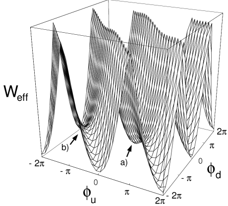
Figure 1: Two flavor effective potential for $q=1$. Indicated points are a) minimum and b) saddle point.

We have checked numerically that in the case $q=1$, $N_{f}=3$ with physical values of the quark masses we stay with one physical vacuum at all values of $\theta$. In particular, no (stable or metastable) vacua appear at $\theta=\pi$. Thus, for $q=1$ the counting of vacua in our approach agrees with that of Ref.[6]. On the other hand, when the Dashen’s constraint [32]

$$m_{u}m_{d}>m_{s}|m_{d}-m_{u}|\;$$ (43)

is satisfied, metastable vacua appear in the vicinity of the point $\theta=\pi$. In particular, in the $SU(2)$ limit $m_{u}=m_{d}\neq m_{s}$ the metastable vacuum exists in a very narrow region near $\theta=\pi$. When $\theta$ becomes exactly equal $\pi$, the two vacua are exactly degenerate. This agrees with the picture of Ref.[6].

Finally, we consider the case $q=1$ with $N_{f}=3$ light flavors of equal masses. In this case, the metastable vacua exist in the extended region of $\theta$ from $\pi/2$ to $3\pi/2$, analogously to what was recently found by Smilga [19] for the VVW potential in the same limit. The resulting picture of the $\theta$ dependence of the vacuum energy is shown in Fig. 2.

Figure 2: Vacuum energy as a function of vacuum angle $\theta$ for the case $q=1$ with $N_{f}=3$ light flavors of equal masses. The solid and dashed lines represent minima and the dotted line is the intermediate saddle point.

Let us now consider the case $q\neq 1$. For the simplest situation of isospin $SU(N_{f})$ symmetry with masses $m_{i}=m\ll\Lambda_{QCD}$, the lowest energy state is described by

$$\phi_{i}^{(l=0)}=\frac{\theta}{N_{f}}\;,\;E_{vac}(\theta)=-E-MN_{f}\cos\left(\frac{\theta}{N_{f}}\right)+O(m_{q}^{2})\;,\;\theta\leq\frac{\pi}{q}\;;$$ (44)

$$\phi_{i}^{(l=1)}=\frac{\theta}{N_{f}}-\frac{2\pi}{qN_{f}}\;,\;E_{vac}(\theta)=-E-MN_{f}\cos\left(\frac{\theta}{N_{f}}-\frac{2\pi}{qN_{f}}\right)+O(m_{q}^{2})\;,\;\frac{\pi}{q}\leq\theta\leq\frac{3\pi}{q}\;;$$ (45)

etc. Thus, the solution (44) coincides with the one obtained by VVW [6] at small $\theta<\pi/q$ up to $O(m_{q}^{2})$ terms. However, at larger values of $\theta$ the true vacuum switches from (44) to (45) with a cusp singularity developing at $\theta=\pi/q$. Here we remind the reader that the “standard” location of the first critical point $\theta=\pi$ corresponds to the particular case $q=1$ in our general formulas. On the contrary, in the scenario [6] the solution remains, if $q\neq 1$, analytic at this point, and for $\pi/q\leq\theta\leq 3\pi/q$ has an energy larger than in (45). On the other hand, if $q=1$, the picture of Ref.[6] is reproduced. Moreover, the number of different solutions (which may or may not be metastable vacua, depending on the signs of second derivatives of the potential) is precisely $N_{f}$ (or $qN_{f}$ if $q\neq 1$) as the phases are defined modulo $2\pi$, and thus only the first $N_{f}$ ($qN_{f}$) terms in the series (44,45) become operative.

The interesting feature of the case $q\neq 1$ is that the vacuum doubling at the points

$$\theta_{k}=(2k+1)\,\frac{\pi}{q}\;\;,\;\;k=0,1,\ldots,p-1$$ (46)

holds irrespective of the values of the light quark masses. This can be seen from the fact that the equations of motion for any two branches with $l=k$ and $l=k+1$ from the set (37) are related by the shift $\theta\rightarrow\theta-2\pi/q$. Thus, the extreme sensitivity of the theory to the values of the light quark masses in the vicinity of the critical point in $\theta$ is avoided in our scenario if $q\neq 1$, while the location of the critical point is given by $\theta_{c}=\pi/q$ instead of the “standard” $\theta_{c}=\pi$. (A similar situation was argued to hold in 2D $CP^{N}$ models on the lattice in the weak coupling limit [29].) Another interesting feature of the scenario $q\neq 1$ is the appearance of metastable vacua which exist for any value of $\theta$, including $\theta=0$. For the physical values of the quark masses, we find $q-1$ additional local minima of the effective chiral potential, which are separated by barriers from the true physical vacuum of lowest energy. For the illustrative purpose, we present in Fig. 3 the effective potential at $\theta=0$ for $q=2,N_{f}=2$.

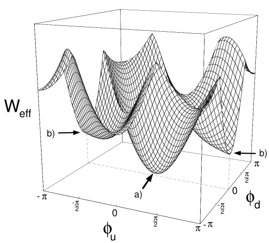
Figure 3: Effective potential for q=2 and $N_{f}=2$. The point indicated as a) is the global minimum. The two points indicated as b) are identified.

The existence of additional local minima of an effective potential for the case $q\neq 1$ leads to the well known phenomenon of the false vacuum decay [33]. For the effective chiral potential (4) this effect and its possible consequences in the context of axion physics were briefly discussed in [34]. Below we present a somewhat more detailed discussion of this issue.

We discuss the problem in a simplified setting by considering the isospin $SU(N_{f})$ limit with equal (and small) fermion masses and taking all chiral phases $\phi_{i}$ equal, $\phi_{i}=\phi$, i.e. restricting our analysis to the “radial” motion in the $\phi$-space. In this setting, the problem becomes tractable in the spirit of Ref.[33]. In what follows, we only consider transitions between a metastable state of lowest energy and the vacuum. To calculate the wall surface tension $\sigma$, it is convenient to shift the vacuum energy by an overall constant such that the metastable state has zero energy, and to rescale and shift the chiral field $\phi\rightarrow(2/f_{\pi}\sqrt{N_{f}})\phi-\pi/(qN_{f})$ in order to have the standard normalization of the kinetic term and symmetrized form of the potential. With these conventions, the effective potential for $\theta=0$ becomes

$$W(\phi)=\left\{\begin{array}[]{ll}E\left[1-\cos\left(\frac{2q\sqrt{N_{f}}}{pf_{\pi}}\phi-\frac{\pi}{p}\right)\right]-Mf(\phi)&\mbox{if $\phi\geq 0$ }\\ E\left[1-\cos\left(\frac{2q\sqrt{N_{f}}}{pf_{\pi}}\phi+\frac{\pi}{p}\right)\right]-Mf(\phi)&\mbox{if $\phi\leq 0$ }\end{array}\right.$$

$$f(\phi)=N_{f}\left[\cos\left(\frac{2}{f_{\pi}\sqrt{N_{f}}}\phi-\frac{\pi}{qN_{f}}\right)-\cos\left(\frac{2\pi}{qN_{f}}\right)\right]$$ (49)

The effective potential (5) has a global minimum at $\phi=\pi f_{\pi}/(2q\sqrt{N_{f}})$ and a local minimum at $\phi=-\pi f_{\pi}/(2q\sqrt{N_{f}})$, with a cusp singularity between them (see Fig. 4). We note that analogous “glued” potentials were discussed for SUSY models in a similar context [5, 8, 9].

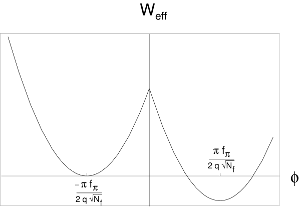
Figure 4: Effective potential at $\theta=0$ for equal chiral phases $\phi=\phi_{u}=\phi_{d}=\phi_{s}$.

A few comments on the above effective potential are in order. First, we note that the potential barrier is high ($\sim\langle G^{2}\rangle$ ) and wide, while the energy splitting for $\theta=0$

$$\Delta E=m_{q}N_{f}\left|\langle\bar{\Psi}\Psi\rangle\right|\left(1-\cos\frac{2\pi}{qN_{f}}\right)+0(m_{q}^{2}),$$ (50)

is numerically small in comparison to the leading term proportional to the gluon condensate. Therefore, the thin wall approximation of Ref.[33] is justified for the physical values of the parameters that enter the effective potential. Indeed, it is easy to check that the necessary condition [33] $3\sigma\mu\gg\Delta E$ (where $\sigma$ is the wall surface tension given by Eq.(53) below, and $\mu$ is the width of the wall) is satisfied to a good accuracy for both alternative choices $p=11N_{c}-2N_{f}=27\,,\,q=8$ or $p=N_{c}=3\,,\,q=1$. (In the latter case, a metastable state does not exist for $N_{f}=3$ and $\theta=0$, but is possible for, say, $N_{f}=5$.) Second, we would like to comment on the meaning of the cusp singularity of the effective potential (5). As was mentioned earlier, the cusp arises as a result of integrating out the “glueball” degrees of freedom, which were carrying information on the topological charge quantization. For an analogous situation in the supersymmetric case, it was argued [9] that the cusp, where the adiabatic approximation breaks down, provides a leading contribution to the wall surface tension. In our case, we expect the difference of the surface tensions for the potential (5) and a potential where the cusp is smoothed to be down by powers of $N_{c}$. The reason is that the domain wall to be discussed below is in fact the $\eta^{\prime}$ wall, while on the other hand, a coupling of the $\eta^{\prime}$ to the glueball fields near the cusp would yield the above suppression.

Explicitly, the domain wall solution corresponding to the effective potential (5) is

$$\phi(x) = \frac{pf_{\pi}}{2q\sqrt{N_{f}}}\left[-\frac{\pi}{p}+4\arctan\left\{\tan\left(\frac{\pi}{4p}\right)\exp[\mu(x-x_{0})]\right\}\right]\;\;,\;\;x<x_{0}$$

$$\phi(x) = \frac{pf_{\pi}}{2q\sqrt{N_{f}}}\left[\frac{\pi}{p}-4\arctan\left\{\tan\left(\frac{\pi}{4p}\right)\exp\left[-\mu(x-x_{0})\right]\right\}\right]\;\;,\;\;x>x_{0}\;,$$ (51)

where $x_{0}$ is the position of the center of the domain wall and

$$\mu\equiv\frac{2q\sqrt{N_{f}}\sqrt{E}}{pf_{\pi}}$$ (52)

is the width of the wall, which turns out to be exactly equal to the $\eta^{\prime}$ mass in the chiral limit, see Eq. (59) below. This suggests the interpretation of the domain wall (5) as the $\eta^{\prime}$ domain wall. The solution (5) as a function of $x-x_{0}$ is shown in Fig. (5). Its first derivative is continuous at $x=x_{0}$, but the second derivative exhibits a jump.

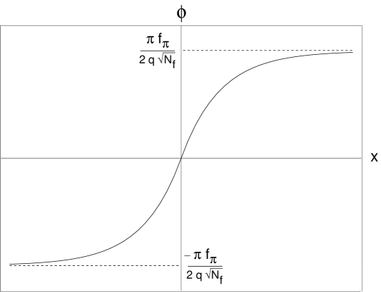
Figure 5: Domain wall profile.

The wall surface tension can be easily calculated from Eq.(5). For $\theta=0$ it is

$$\sigma=\frac{4p}{q\sqrt{N_{f}}}f_{\pi}\sqrt{\langle\frac{b\alpha_{s}}{32\pi}G^{2}\rangle}\,\left(1-\cos\frac{\pi}{2p}\right)+0(m_{q}f_{\pi}^{2}).$$ (53)

Eq.(53) should be compared with the formula

$$\sigma=3\sqrt{2}\left(1-\frac{\pi}{3\sqrt{3}}\right)m_{\pi}f_{\pi}^{2}.$$ (54)

found by Smilga [19] for the the wall surface tension at $\theta\simeq\pi$ for the VVW potential [6] with $N_{f}=3$ with equal fermion masses. A distinct difference between these two cases is the absence of the chiral suppression $\sim m_{q}$ in Eq.(53), which apparently would make penetration through the barrier even more difficult in comparison to the VVW potential. Another difference is the large $N_{c}$ behavior of Eqs. (53) and (54). For fixed $m_{q}\neq 0$, the surface tension scales as $O(N_{c})$ for both cases, while in the limit $m_{q}\rightarrow 0$ first and then $N_{c}\rightarrow\infty$ the surface tension vanishes for Eq. (54) and scales as $N_{c}^{1/2}$ for Eq. (53).

The quasiclassical formula for the decay rate per unit time per unit volume is [33]

$$\Gamma\propto\exp\left(-\frac{27\pi^{2}\sigma^{4}}{2(\Delta E)^{3}}\right)\equiv\exp(-S_{4}).$$ (55)

Using (54), one finds that in the VVW scenario the lifetime of the metastable state at zero temperature is much larger than the age of the Universe [19]. In our case, we find a very different result

$$S_{4}=\frac{3^{3}\cdot 2^{7}\cdot\pi^{2}p^{4}}{q^{4}N_{f}^{5}}\,\frac{f_{\pi}^{4}E^{2}}{M^{3}}\,\frac{\left(1-\cos\frac{\pi}{2p}\right)^{4}}{\left(1-\cos\frac{2\pi}{qN_{f}}\right)^{3}}\simeq\frac{27}{256}\,\frac{\pi^{4}q^{2}N_{f}}{p^{4}}\,\frac{f_{\pi}^{4}\langle\frac{b\alpha_{s}}{32\pi}G^{2}\rangle^{2}}{m_{q}^{3}\left|\langle\bar{\Psi}\Psi\rangle\right|^{3}}\;.$$ (56)

Eq.(56) shows that the false vacuum decay is suppressed parametrically by a factor $\sim(\Lambda_{QCD}/m_{q})^{3}$, which should be compared to a factor $\sim(\Lambda_{SYM}/m_{g})^{3}$ in the soft SUSY breaking scheme [8, 16]. While the latter ceases to yield a suppression with approaching the decoupling limit $m_{g}\gg\Lambda_{SYM}$, the former is a real suppression factor for QCD. As should be expected, it tends to infinity (i.e. vacua become stable) when $m_{q}$ goes to zero. On the other hand, Eq.(56) shows that the parametric suppression of the decay is largely overcome due to a numerical enhancement. The latter depends crucially on the particular values of the integers $p,q$. In particular, for our favorite choice $p=11N_{c}-2N_{f},q=8$, Eq.(56) yields a factor $\simeq 10$, while for $p=N_{c},q=1$ (as motivated by SUSY, see Sect.3) it is approximately two orders of magnitude larger, but still much smaller than the estimate of [19] for the VVW potential. For a discussion of these results, see [34].

To conclude this section, we would like to note that there also exist other domain walls interpolating between different local minima of the effective potential (4). The surface tension $\sigma$ and decay rate $\Gamma$ for these walls strongly depend on the vacuum states connected by the wall.

6 Pseudo-goldstone bosons at different $\theta$ angles

In this section we address a few related questions. First, we discuss the calculation of the $\eta^{\prime}$ mass from the effective chiral Lagrangian (4) and show that the main contribution to $m_{\eta^{\prime}}$ is given by the conformal anomaly. We also calculate the $\theta$ dependence of the $\eta^{\prime}$ mass. Furthermore, it will be shown that for non-zero values of $\theta$, the pseudo-goldstone bosons cease to be the pure pseudoscalars, but in addition acquire scalar components.

To study the properties of the pseudo-goldstone bosons, we parametrize the chiral matrix (10) in the form

$$U=U_{0}\,\exp\left[i\sqrt{2}\,\frac{\pi^{a}\lambda^{a}}{f_{\pi}}+i\frac{2}{\sqrt{N_{f}}}\frac{\eta^{\prime}}{f_{\eta^{\prime}}}\right]\;,$$ (57)

where $U_{0}$ solves the minimization equations for the effective potential (4), and the fields $\pi^{a}\,,\,\eta^{\prime}$ all have vanishing vacuum expectation values. A simple calculation of the matrix of second derivatives yields the following result for the mass matrix for an arbitrary value of $\theta$:

$$m_{33}^{2} = \frac{2}{f_{\pi}^{2}}(M_{u}\cos\phi_{u}+M_{d}\cos\phi_{d})$$

$$m_{88}^{2} = \frac{2}{3f_{\pi}^{2}}(M_{u}\cos\phi_{u}+M_{d}\cos\phi_{d}+4M_{s}\cos\phi_{s})$$

$$m_{11}^{2} = 4\left(\frac{q}{p}\right)^{2}\,\frac{E}{f_{\eta^{\prime}}^{2}}\,N_{f}\,\cos\left(-\frac{q}{p}\theta+\frac{q}{p}\sum\phi_{i}+\frac{2\pi l}{p}\right)+\frac{4}{N_{f}}\frac{1}{f_{\eta^{\prime}}^{2}}\sum_{i=u,d,s}M_{i}\cos\phi_{i}$$

$$m_{38}^{2} = m_{83}^{2}=\frac{2}{\sqrt{3}f_{\pi}^{2}}\left(M_{u}\cos\phi_{u}-M_{d}\cos\phi_{d}\right)$$ (58)

$$m_{31}^{2} = m_{13}^{2}=2\sqrt{\frac{2}{N_{f}}}\frac{1}{f_{\pi}f_{\eta^{\prime}}}\left(M_{u}\cos\phi_{u}-M_{d}\cos\phi_{d}\right)$$

$$m_{81}^{2} = m_{18}^{2}=2\sqrt{\frac{2}{3N_{f}}}\frac{1}{f_{\pi}f_{\eta^{\prime}}}\left(M_{u}\cos\phi_{u}+M_{d}\cos\phi_{d}-2M_{s}\cos\phi_{s}\right)\;,$$

where $\phi_{i}$ are solutions of the minimization equation stemming from Eq.(37). They depend on $\theta$ as well as other parameters of the effective Lagrangian. If the $\pi^{0}-\eta-\eta^{\prime}$ mixing is neglected, $m_{11}$ coincides with the physical mass of the $\eta^{\prime}$. For $\theta=0$ and the particular choice $p=3b,q=8$, we reproduce in this limit the relation given in [3]:

$$f_{\eta^{\prime}}^{2}\,m_{\eta^{\prime}}^{2}=\frac{8}{9b}N_{f}\langle\frac{\alpha_{s}}{\pi}\,G^{2}\rangle-\frac{4}{N_{f}}\sum_{u,d,s}m_{i}\langle\bar{\Psi}_{i}\Psi_{i}\rangle+O(m_{q}^{2})\;.$$ (59)

(The choice $p=N_{c},q=1$ would produce a numerically close result.) This mass relation for the $\eta^{\prime}$ appears reasonable phenomenologically. Note that, according to Eq.(59), the strange quark contributes 30-40 % of the $\eta^{\prime}$ mass. This may lead us to expect that chiral corrections $O(m_{s}^{2})$ could be quite sizeable. We also note that in the formal limit $N_{c}\rightarrow\infty,m_{q}\rightarrow 0$ Eq.(59) coincides with the relation obtained in [12]. In this limit $m_{\eta^{\prime}}^{2}$ scales as $N_{f}/N_{c}$, in agreement with Ref. [20]. In the different limit when $N_{c}$ goes to infinity at fixed non-zero $m_{q}$, the result is $m_{\eta^{\prime}}^{2}=O(m_{q}N_{c}^{0})$, as for ordinary pseudo-goldstone bosons. As for the $\theta$ dependence of the $\eta^{\prime}$ mass in the same limit, it is given by the third of Eq.(6) where the phases $\phi_{i}$ implicitly depend on $\theta$ through the minimization equation for the effective potential (4).

The mass matrix (6) can be used to study the mixing between pseudo-goldstone bosons (including also its $\theta$ dependence). Let us consider the simplest case of the $\eta-\eta^{\prime}$ mixing which decouples from the $\pi^{0}$ in the isospin limit $m_{u}=m_{d}=m$, $\langle\bar{d}d\rangle=\langle\bar{u}u\rangle=\langle\bar{q}q\rangle$. For the case $\theta=0$, it is easy to verify that the mixing matrix

$$m_{\eta-\eta^{\prime}}^{2}=\left(\begin{array}[]{cl}-\frac{4}{3f_{\pi}^{2}}(2m_{s}\langle\bar{s}s\rangle+m\langle\bar{q}q\rangle)&\frac{4\sqrt{2}}{\sqrt{3}f_{\pi}f_{\eta^{\prime}}}(m_{s}\langle\bar{s}s\rangle-m\langle\bar{q}q\rangle)\\ \frac{4\sqrt{2}}{\sqrt{3}f_{\pi}f_{\eta^{\prime}}}(m_{s}\langle\bar{s}s\rangle-m\langle\bar{q}q\rangle)&-\frac{4}{3f_{\eta^{\prime}}^{2}}\sum m_{i}\langle\bar{\Psi}_{i}\Psi_{i}\rangle+\frac{N_{f}b}{8}\left(\frac{q}{p}\right)^{2}\,\frac{\langle(\alpha_{s}/\pi)G^{2}\rangle}{f_{\eta^{\prime}}^{2}}\end{array}\right)$$ (62)

coincide with an accuracy $O(m_{q}^{2})$ with the matrix given by Veneziano [20]

$$m_{\eta-\eta^{\prime}}^{2}=\left(\begin{array}[]{cl}\frac{1}{3}(4m_{K}^{2}-m_{\pi}^{2})&-\frac{2\sqrt{2}}{3}(m_{K}^{2}-m_{\pi}^{2})\\ -\frac{2\sqrt{2}}{3}(m_{K}^{2}-m_{\pi}^{2})&\frac{2}{3}m_{K}^{2}+\frac{1}{3}m_{\pi}^{2}+\frac{\chi}{N_{c}}\end{array}\right)$$ (65)

with the only (but important) difference that the topological susceptibility $\sim\chi$ in pure YM theory in the latter is substituted by the term proportional to the gluon condensate in real QCD in the former. For the particular values $p=3b=11N_{c}-2N_{f},q=8$, we may write down a QCD analog of the Witten-Veneziano formula:

$$\langle\frac{\alpha_{s}}{\pi}G^{2}\rangle=\frac{3b}{8}f_{\eta^{\prime}}^{2}\,(m_{\eta^{\prime}}^{2}+m_{\eta}^{2}-2m_{K}^{2})+O(m_{q}^{2})\;.$$ (66)

This relation generalizes Eq.(59) as it now includes the $\eta-\eta^{\prime}$ mixing.

Eqs. (6) can also be used to study other problems related to the physics of the pseudo-goldstone bosons. In particular, we may find the mixing angles in the system $\pi^{0}-\eta-\eta^{\prime}$ at zero and non-zero angles $\theta$. Instead of discussing these more phenomenological issues, we here would like to address another interesting aspect of the corresponding physics. Namely, we would like to show that the neutral pseudo-goldstone bosons in the $\theta$-vacuum cease to be the pure pseudoscalars, but instead become mixtures of the scalar and pseudoscalar states. To show this, we note that the result found for the quark condensates in the $\theta$-vacuum

$$\langle\bar{\Psi}_{Li}^{\prime}\Psi_{Rj}^{\prime}\rangle_{\theta}\equiv\langle\bar{\Psi}_{Li}\Psi_{Rj}\rangle_{\theta=0}\,e^{i\phi_{i}}$$ (67)

can be represented as a chiral rotation of the usual $\theta=0$ vacuum:

$$\Phi^{\prime}=U_{R}\Phi U_{L}^{+}\;\;,\;\;\Phi_{ij}=\langle\bar{\Psi}_{Li}\Psi_{Rj}\rangle_{\theta=0}\;.$$ (68)

Under such a rotation, the quark fields transform as

$$\Psi_{Ri}^{\prime}=\left(U_{R}\right)_{ik}\Psi_{Rk}\;\;,\;\;\Psi_{Lj}^{+^{\prime}}=\Psi_{Lk}^{+}\left(U^{+}\right)_{kj}\;.$$ (69)

In the “rotated” basis, the spin content of the pseudo-goldstone bosons is the standard one. However, the relations (69) imply that it will generally have a different form in terms of the original unrotated fields. From Eqs.(67,68) we obtain

$$\left(U_{R}U_{L}^{+}\right)_{ii}=e^{i\phi_{i}}\;\;(no\;\;sum\;\;over\;\;i)\;\;\Rightarrow\left(U_{R}\right)_{ik}=\delta_{ik}e^{\frac{i}{2}\phi_{i}}\;\;,\;\;\left(U_{L}^{+}\right)_{kj}=\delta_{kj}e^{\frac{i}{2}\phi_{i}}\;.$$ (70)

Let us consider e.g. the $\pi^{0}$ field in the $\theta$-vacuum. In the ”rotated” basis, it has the usual spin content. Using the correspondence (69,70), we obtain

$$|\pi^{0}\rangle\sim|\bar{u}^{\prime}i\gamma_{5}u^{\prime}-\bar{d}^{\prime}i\gamma_{5}d^{\prime}\rangle=\cos\phi_{u}\,|\bar{u}i\gamma_{5}u\rangle-\sin\phi_{u}\,|\bar{u}u\rangle-(u\leftrightarrow d)$$ (71)

Eq.(71) illustrates the phenomenon announced in the beginning of this section: In the presence of a non-zero angle $\theta$, the pseudo-goldstone bosons cease to be the pure pseudoscalars, but in addition acquire scalar components. Although in reality $\theta$ is extremely close to zero, this observation is not only of academic interest. The point is that in heavy ion collisions one can effectively create, in principle, an arbitrary value of $\theta$ [34]. In these circumstances, the scalar admixture in the pseudo-goldstones would be quite large, and probably could play an important role in dynamics.

7 Further applications and speculations

7.1 Axion potential from effective Lagrangian

One of the interesting implications of the present effective Lagrangian approach concerns the possibility to construct a realistic axion potential [34] consistent with the known Ward identities of QCD. This may be achieved due to the one-to-one correspondence between the form of the axion potential $V(a)$ and the vacuum energy $E_{vac}(\theta)$ as a function of the fundamental QCD parameter $\theta$. Indeed, the axion solution of the strong CP problem suggests (see e.g. [36]) that $\theta$ parameter in QCD is promoted to the dynamical axion field $\theta\rightarrow a(x)/f_{a}$, and the QCD vacuum energy $E_{vac}(\theta)$ becomes the axion potential $V(a)$. Therefore, the problem of analysing $V(a)$ amounts to the study of $E_{vac}(\theta)$ in QCD without the axion, which is exactly the problem addressed above in the present paper.

Both the local and global properties of the axion potential can be analysed with this approach. As for the former, we note that, as all dimensionful parameters in our effective Lagrangian are fixed in terms of the QCD quark and gluon condensate, the temperature dependence of the axion mass (and of the entire axion potential) can be related with that of the QCD condensates whose temperature dependence is understood (from lattice or model calculations).

In particular, the axion mass, which is defined as the quadratic coefficient in the expansion of the function $E_{vac}(\theta)$ at small $\theta$, is proportional to the chiral condensate: $m_{a}^{2}(T)\sim m_{q}\langle 0|\bar{\Psi}\Psi|0\rangle_{T}/f_{a}^{2}$. Therefore, $m_{a}^{2}(T)$ is known as long as $\langle 0|\bar{\Psi}\Psi|0\rangle_{T}$ is known. This statement is exact up to the higher order corrections in $m_{q}$. We neglect these higher order corrections everywhere for $T\leq T_{c}$ ($T_{c}\simeq 200\,MeV$ is the critical temperature), where the chiral condensate is nonzero and gives the most important contribution to $m_{a}$. For the particular case $N_{f}=2$ one expects a second order phase transition and, therefore, $m_{a}^{2}\sim\frac{m_{q}}{f_{a}^{2}}\langle 0|\bar{\Psi}\Psi|0\rangle\sim|T_{c}-T|^{\beta}$ for $T$ near $T_{c}\simeq 200\,MeV$. This is exactly where the axion mass does “turn on”. The critical exponent in this case $\beta\simeq 0.38$, see e.g. recent reviews [37] for a general discussions of the QCD phase transitions.

The global (topological) structure of the axion potential appear to be rather complicated, in contrast to what could be expected according to simple model potentials such as $V(a)=m_{a}^{2}a^{2}/2$ or $V(a)\sim\cos(a/f_{a})$. In particular, it admits the appearance of additional local minima of an effective potential. Thus, the axion potential may become a multi-valued function, i.e. there would be two different values of the axion potential $V_{1,2}(\theta=a/f_{a})$ for a fixed $\theta$, which differ by the phase of the chiral field. For the VWW potential, this happens only at $\theta\sim\pi$ for a small isospin breaking, while for the effective potential (4) with $q\neq 1$ metastable vacua exist for any $\theta$, similarly to the case of a softly broken SUSY. Interpolating between two minima is the domain wall that was described in Sect. 5. We stress that it is not an axion domain wall, as the value of $\theta$ does not change in this transition. Similar domain walls which separate vacua with different phases of the gluino condensate have been recently discussed [8, 9] for the SUSY models. The appearance of such a domain wall implies an interesting dynamics which develops at temperatures below the chiral phase transition, which still has to be explored.

7.2 Axially disoriented chiral condensate and axion search at RHIC

Another interesting phenomenon amenable to an analysis within the effective Lagrangian framework is the possibility of production of finite regions of $\theta\neq 0$ vacua in heavy ion collisions [34], where the chiral fields are misaligned from the true vacuum in the axial $U_{A}(1)$ direction. This is somewhat analogous to the production of the disoriented chiral condensate (DCC) with a “wrong” isospin direction (see e.g. [38] for a review).

Let us briefly recall the reason as to why the DCC could be produced and observed in heavy ion collisions. The energy density of the DCC is determined by the mass term:

$$E_{\phi}=-\frac{1}{2}Tr(MU+M^{+}U^{+})=-2m|\langle\bar{\Psi}\Psi\rangle|\cos(\phi)$$ (72)

where we put $m_{u}=m_{d}=m$ for simplicity, and $\phi$ stands for the misalignment angle. Thus, the energy difference between the misaligned state and true vacuum with $\phi=0$ is small and proportional to $m_{q}$. Therefore, the probability to create a state with an arbitrary $\phi$ at high temperature $T\sim T_{c}$ is proportional to $\exp[-V(E_{\phi}-E_{0})/T]$ and depends on $\phi$ only very weakly, i.e. $\phi$ is a quasi-flat direction. Just after the phase transition when $\langle\bar{\Psi}\Psi\rangle$ becomes nonzero, the pion field begins to roll toward $\phi=0$, and of course overshoots $\phi=0$. Thereafter, $\phi$ oscillates. One should expect coherent oscillations of the $\pi$ meson field which would correspond to a zero-momentum condensate of pions. Eventually, these classical oscillations produce the real $\pi$ mesons which hopefully can be observed at RHIC.

We now wish to generalize this line of reasoning to the case when the chiral phases are misaligned in the $U_{A}(1)$ direction as well. For arbitrary phases $\phi_{i}$ the energy of a misaligned state differs by a huge amount $\sim E$ from the vacuum energy. Therefore, apparently there are no quasi-flat misaligned $U_{A}(1)$ directions among $\phi_{i}$ coordinates, which would lead to long wavelength oscillations with production of a large size domain. However, when the relevant combination $(\sum_{i}\phi_{i}-\theta)$ from Eq.(4) is close by an amount $\sim O(m_{q})$ to its vacuum value, a Boltzmann suppression due to the term $\sim E$ is absent, and an arbitrary misaligned $|\theta\rangle$-state can be formed. In this case for any $\theta$ the difference in energy between the true $|\theta\rangle$ vacuum and a misaligned $|\theta\rangle$- state (when the $\phi_{i}$ fields are not yet in their final positions $\overline{\phi_{i}(\theta)}$) is proportional to $m_{q}$ and very small in close analogy to the DCC case.

Once formed, such a domain with $\theta\neq 0$ could serve as a source of axions, thus suggesting a new possible strategy for the axion search. Below we would like to sketch this idea, referring the interested reader to Ref. [34] for more details.

It is well known that $\theta$ is a world constant in the usual infinite volume equilibrium formulation of a field theory. The superselection rule ensures that the only way to change $\theta$ under these conditions is to have an axion in the theory. However, due to the fact that we do not expect to create an equilibrium state with an infinite correlation length in heavy ion collisions, the decay of a $|\theta\rangle$-state will also occur due to the Goldstone $U$ fields with specific $CP$-odd correlations. Therefore, two mechanisms of the relaxation of a $|\theta\rangle$-state to the vacuum would compete: the axion one and the standard decay to the Goldstone bosons. In the large volume limit if a reasonably good equilibrium state with a large correlation length is created, the axion mechanism would win; otherwise, the Goldstone mechanism would win. In any case, the result of the decay of a $|\theta\rangle$-state would be very different depending on the presence or absence of the axion field in Nature. Provided the axion production is strong enough, the axion could be detected by using their property of conversion into the photons in an external magnetic field [41]. Thus, heavy ion collisions may provide us with a way to finally catch the so far elusive axion.

7.3 Early Universe during the QCD epoch

As was discussed in Sect. 5, the effective Lagrangian approach developed in this paper predicts the existence of the domain wall excitations in QCD at zero temperature. One may expect that these domain walls appear also for non-zero temperatures $T<T_{c}$ where $T_{c}$ is the temperature of the chiral phase transition. If so, it would be very interesting to study this dynamics in the cosmological context. Here we only mention that the walls discussed above are harmless cosmologically as they decay in a proper time [34]. On the other hand, as was noted in [34], the dynamics of the decaying domain walls is an out-of-equilibrium process with $100\%$ violation of $CP$ invariance. This is because the phase of the chiral condensate in the metastable vacuum is nonzero and of order 1, that leads to violation of $CP$ even if $\theta=0$. (This is not at variance with the Vafa-Witten theorem [42] which refers to the lowest energy state only.) It was speculated in [34] that such effects could lead to a new mechanism for baryogenesis at the QCD scale. Indeed, it appears that all three famous Sakharov criteria [43] could be satisfied in the decay of a metastable state discussed above:
1. Such a metastable state is clearly out of thermal equilibrium;
2. CP violation is unsuppressed and proportional to $m_{u}m_{d}m_{s}\bar{\theta}_{eff},~{}\bar{\theta}_{eff}\sim 1$. As is known, this is the most difficult part to satisfy in the scenario of baryogenesis at the electroweak scale within the standard model for CP violation;
3. The third Sakharov criterion is violation of the baryon $(B)$ number. Of course, the corresponding U(1) is an exact global symmetry of QCD. However, a “spontaneous” baryon number non-conservation could arise in this dynamics as a result of interactions of fermions with the domain wall. In this case, baryogenesis at the QCD scale is feasible. One possible scenario [44] of such a “spontaneous” baryogenesis with zero net baryon asymmetry is a mechanism based on a charge separation, when the anti-baryon charge is concentrated on the surface of balls of the metastable vacuum produced in evolution of domain walls (B-shells). Rough estimates [44] show that the observed ratio $(n_{B}-n_{\bar{B}})/s\sim 10^{-9}$ can be easily reproduced in this scenario. Surprisingly, the energy density $\Omega_{\bar{B}}$ associated with these B-shells can be close to unity. Therefore, they can be considered as candidates for dark matter. We would like to emphasize that each step in such a scenario for baryogenesis at the QCD scale could be, in principle, experimentally tested at RHIC.

Appendix: Fixing $p/q$ by the “integrating in”

The purpose of this appendix is to suggest a method which allows one to fix the number $p/q$ that appears in the effective potential (2), provided two plausible assumptions are made. One of them is insisting on the standard form of the fermion mass term in the effective potential, while the other one is the hypothesis of preserving the holomorphic properties when a heavy fermion is integrated in/out, see below. The approach developed below closely follows the method of [10] where a similar problem was addressed for the effective Lagrangian [4] for pure YM theory. The essence of this method is to consider QCD with light fermions as a low energy limit of a theory including in addition a heavy fermion, and to construct an effective Lagrangian for the latter theory starting from the effective Lagrangian (2). As will be shown below, a relation between the holomorphic and “topological” properties of two Lagrangians is non-trivial, and allows one to fix the crucial parameter $\xi=q/(2p)$ entering Eq.(2).

The task of constructing such an effective Lagrangian for the theory with a heavy fermion is achieved by using the “integrating in” technique, developed in the context of SUSY theories in Ref.[22] and reviewed by Intriligator and Seiberg [23]. The integrating in procedure can be viewed as a method of introducing an auxiliary field into the effective Lagrangian for QCD with light flavors. Using the renormalization group properties of the QCD effective Lagrangian in the chiral limit $m_{q}\rightarrow 0$, the latter is extended to include the auxiliary field $T$, which will be later on identified with the chiral combination $\bar{Q}_{L}Q_{R}$ of a heavy fermion.

To conform with the notation and terminology of Ref.[22], we will call QCD with light quarks and the theory with a heavy fermion the d-theory (from “downstairs”) and the u-theory (from “upstairs”), respectively. The effective potential of the d-theory is then $W_{d}+W_{d}^{+}$ with (see Eq.(13))

$$W_{d}(h,U)=\frac{1}{4}\frac{q}{p}h\,Log\left[\left(\frac{h}{c\Lambda_{QCD}^{4}}\right)^{p/q}\frac{Det\,U}{e^{-i\theta}}\right]-\frac{1}{2}Tr\,MU\;,$$ (A.1)

(here $c$ is a dimensionless numerical coefficient), and the summation over all branches of the logarithm in the partition function is implied. In this section Eq.(A.1) will be understood as representing a branch (section) of the multi-valued effective potential, which corresponds to a lowest energy state for small $\theta\ll\pi$. As was shown in [4, 10], this section corresponds to the principal branch of the rational function in the logarithm in Eq.(A.1).

We now want to relate [17, 22] the dimensional transmutation parameter $\Lambda_{QCD}$ of the d-theory to the scale parameter $\Lambda_{QCD+1}$ of the u-theory including a heavy quark of mass $m\gg\Lambda_{QCD},\Lambda_{QCD+1}$. We assume both parameters to be defined in the $\overline{MS}$ scheme, in which no threshold factors arise in corresponding matching conditions. The matching condition then follows from the standard one-loop relations

$$\Lambda_{QCD} = M_{0}\exp\left(-\frac{8\pi^{2}}{b_{QCD}g^{2}(M_{0})}\right)\;\;,\;\;b_{QCD}\equiv b=\frac{11}{3}\,N_{c}-\frac{2}{3}N_{f}\;,$$

$$\Lambda_{QCD+1} = M_{0}\exp\left(-\frac{8\pi^{2}}{b_{QCD+1}g^{2}(M_{0})}\right)\;\;,\;\;b_{QCD+1}=\frac{11}{3}\,N_{c}-\frac{2}{3}(N_{f}+1)\;,$$ (A.2)

and the requirement that the coupling constants of the d- and u- theories coincide at the decoupling scale $M_{0}=m$. We obtain

$$\Lambda_{QCD}^{4}=\Lambda_{QCD+1}^{4}\left(\frac{m^{2}}{\Lambda_{QCD+1}^{2}}\right)^{4/(3b)}\;,$$ (A.3)

As was explained in Ref.[17, 22, 23], Eq.(A.3) reflects the fact that, for fixed $\Lambda_{QCD+1}$, the scale parameter $\Lambda_{QCD}$ characterizes the low energy theory surviving below the scale $m$, and thus depends on $m$. In this sense, the constant in the logarithm in Eq.(A.1) also depends on $m$

$$(c\Lambda_{QCD}^{4})^{p/q}=(c\Lambda_{QCD+1}^{4})^{p/q}\,\left(\frac{m}{\Lambda_{QCD+1}}\right)^{8p/(3bq)}\;.$$ (A.4)

Following Ref.[22], we now wish to consider (a particular branch of) the effective potential (A.1) as the result of integrating out the auxiliary field $T$ in the new effective potential $W\equiv W_{u}-mT$ which corresponds to the u-theory: $W_{d}(h,m)=W(h,m,\langle T\rangle)$, or

$$W_{d}=[W_{u}-mT]_{\langle T\rangle}\;,$$ (A.5)

where $\langle T\rangle$ is a solution of the classical equation of motion for the auxiliary field $T$ :

$$\frac{\partial W_{u}}{\partial T}-m=0\;.$$ (A.6)

Let us note that, according to Eq.(A.5), $W_{d}$ should depend holomorphically on $\langle T\rangle$. Our assumption is that this is only possible if an effective potential $W$ of the u-theory is itself holomorphic in the field $T$. Furthermore, one can see that Eqs. (A.5),(A.6) actually define the potential $W_{d}$ as the Legendre transform of $W_{u}$. Therefore we can find the unknown function $W_{u}$ from the known potential $W_{d}$ by the inverse Legendre transform:

$$W_{u}=[W_{d}+mT]_{\langle m\rangle}\;,$$ (A.7)

where $\langle m\rangle$ solves the equation

$$\frac{\partial}{\partial m}\,(W_{d}+mT)=0\;.$$ (A.8)

Eq.(A.8) can be considered as an equation of motion for the auxiliary “field” $m$. It is important to note that Eqs. (A.5 - A.8) imply that $m$ should be treated as a complex parameter to preserve the holomorphic structure of Eq.(A.1). When substituted in Eq.(A.7), a solution $\langle m\rangle$ of Eq.(A.8) defines the potential $W_{u}(h,T,\langle m\rangle)$. When this function is found, the effective potential $W$ of the u-theory is defined by the relation

$$W(h,T,m)=W_{u}(h,T,\langle m\rangle)-mT\;,$$ (A.9)

in accord with Eq.(A.5).

The solution of Eq.(A.8) is easy to find using Eqs. (A.1), (A.4) :

$$\langle m\rangle=\frac{2}{3b}\,\frac{h}{T}\;.$$ (A.10)

Thus, Eq.(A.7) yields

$$W_{u}=-\frac{1}{4}\,\frac{q}{p}\,h\log\left[\left(\frac{c\Lambda_{QCD+1}^{4}}{h}\right)^{p/q}\left(\frac{2}{3b}\,\frac{h}{\Lambda_{QCD+1}T}\right)^{8p/(3bq)}\frac{e^{-i\theta}}{Det\,U}\right]+\frac{2}{3b}\,h\;.$$ (A.11)

Finally, Eq.(A.9) results in the effective potential of the u-theory

$$W=\frac{1}{4}\,\frac{q}{p}\,h\log\left[\left(\frac{h}{c\Lambda_{QCD+1}^{4}}\right)^{(1-8/3b)p/q}\left(\frac{3b}{2}\,\frac{T}{c\Lambda_{QCD+1}^{3}}\right)^{8p/(3bq)}\frac{Det\,U}{e^{-i\theta}}\right]+\frac{2}{3b}\,h-mT\;.$$ (A.12)

We expect this effective Lagrangian to describe QCD with light quarks and the additional heavy quark, corresponding to the field $T$, such that integrating out $T$ brings us back to the effective Lagrangian (A.1) for QCD. Indeed the equation of motion for the field $T$ stemming from the effective potential (A.12) reads

$$m\langle T\rangle=\frac{2}{3b}\,h\;.$$ (A.13)

Inserting this classical vacuum expectation value (VEV) back to Eq.(A.12) (i.e. integrating out the field $T$), we reproduce the effective potential of the d-theory, Eq.(A.1). Note that as Eq.(A.13) should preserve the $N_{c}$ counting rule, we obtain $\langle h\rangle\sim N_{c}^{2}$ , $b\sim N_{c}$, $\langle T\rangle\sim N_{c}$. The $N_{c}$ dependence of the VEV $\langle T\rangle$ is consistent with the identification $\langle T\rangle\sim\langle\bar{Q}_{L}Q_{R}\rangle$ which will be suggested below.

To identify the field $T$ of the effective theory with a corresponding operator of the fundamental theory, we note the following. As is seen from (A.13), $T$ has dimension 3, and thus should describe the VEV of an operator bilinear in the heavy quark fields. Furthermore, as long as $m$ is effectively considered as a complex parameter, this operator can only be $\bar{Q}_{L}Q_{R}$ or $\bar{Q}_{R}Q_{L}$, in accord with the structure of the mass term in the underlying fundamental theory. Comparing Eq.(A.13) with the relation between the VEV’s in the underlying theory:

$$\langle m\bar{Q}_{L}Q_{R}\rangle=\frac{\alpha_{s}}{24\pi}\left(-G^{2}+i\,\frac{3}{2}G\tilde{G}\right)\;,$$ (A.14)

and recalling the definition of the fields $h\,,\,H$, we conclude that

$$\xi=\frac{4}{3b}\;\;,\;\;\frac{q}{p}=\frac{8}{3b}\;\;;\;\;\langle T\rangle=\langle\bar{Q}_{L}Q_{R}\rangle\;.$$ (A.15)

We thus see that the introduction of the heavy quark into the effective theory fixes the parameter $\xi$ which enters the effective Lagrangian (A.1) for QCD. This has been obtained by the matching the local holomorphic properties of the d- and u-theories within the integrating in procedure. As was shown in [10], the matching of the two theories can also be considered at the level of global quantization rules for the $h\,,\,\bar{h}$ fields which, for general values of $p/q$, are different for the theories described by Eqs. (A.1) and (A.12). This matching agrees with the result (A.15), and provides a self-consistency check of the whole procedure of using the integrating in procedure to fix the parameter $q/p=2\xi$ which enters the effective potential (2). Finally, we note that the correspondence

$$mT\Leftrightarrow m\bar{Q}_{L}Q_{R}\;\;,\;\;\bar{m}\bar{T}\Leftrightarrow m\bar{Q}_{R}Q_{L}\;.$$ (A.16)

between the operators of the effective and underlying theories has the same meaning as Eqs.(1), i.e. the classical field $T$ describes the VEV of the chiral combination $\bar{Q}_{L}Q_{R}$ of the full (QCD +1) theory.

References

- [1] G. Veneziano and S. Yankielowicz, Phys. Lett. 113B (1982) 231.
- [2] T. Taylor, G. Veneziano and S. Yankielowicz, Nucl. Phys. B218 (1983) 439.
- [3] I. Halperin and A. Zhitnitsky, hep-ph/9803301.
- [4] I. Halperin and A. Zhitnitsky, hep-ph/9711398, Phys. Rev. D58 (1998), to appear.
- [5] A. Kovner and M. Shifman, Phys. Rev. D56 (1997) 2396, hep-th/9702174.
-
[6]
E. Witten, Ann. Phys. 128 (1980) 363.
P. Di Vecchia and G. Veneziano, Nucl. Phys. B171 (1980) 253. -
[7]
C. Rosenzweig, J. Schechter and G. Trahern, Phys.
Rev. D21 (1980) 3388.
P. Nath and A. Arnowitt, Phys. Rev. D23 (1981) 473. - [8] A. Kovner, M. Shifman and A. Smilga, Phys. Rev. D56 (1997) 7978, hep-th/9706089.
- [9] I. Kogan, A. Kovner and M. Shifman, Phys. Rev. D57 (1998) 5195, hep-th/9712046.
- [10] I. Halperin and A. Zhitnitsky, hep-th/9802095.
- [11] V.A. Novikov, M.A. Shifman, A.I. Vainshtein and V.I. Zakharov, Nucl. Phys. B191 (1981) 301.
- [12] I. Halperin and A. Zhitnitsky, Mod. Phys. Lett. A13 (1998) 1955, hep-ph/9707286.
- [13] H. Gomm, P. Jain, R. Johnson and J. Schechter, Phys. Rev. D33 (1986) 801.
-
[14]
R.J. Crewther, Phys. Lett. 70B (1977) 349.
M.A. Shifman, A.I. Vainshtein, and V.I. Zakharov, Nucl. Phys. B166 (1980) 493. - [15] A. Masiero and G. Veneziano, Nucl. Phys. B249 (1985) 593.
- [16] M. Shifman, hep-ph/9704114.
- [17] M.A. Shifman and A.I. Vainshtein, Nucl. Phys. B296 (1988) 445.
- [18] F. Sannino and J. Schechter, Phys. Rev. D57 (1998) 170, hep-th/9708113.
- [19] A.V. Smilga, hep-ph/9805214.
-
[20]
E. Witten, Nucl. Phys. B156 (1979) 269.
G. Veneziano, Nucl. Phys. B159 (1979) 213. - [21] J.H. Kühn and V.I. Zakharov, Phys. Lett. B252 (1990) 615.
-
[22]
K. Intriligator, R.G. Leigh, and N. Seiberg,
Phys. Rev. D50 (1994) 1092.
K. Intriligator, Phys. Lett. B336 (1994) 409. - [23] K. Intriligator and N. Seiberg, hep-th/9509096.
- [24] E. Witten, hep-th/9807109.
-
[25]
J. Maldacena, hep-th/9711200.
S. Gubser, I.R. Klebanov and A.M. Polyakov, hep-th/9802109.
E. Witten, hep-th/9802150, hep-th/9803131. - [26] D. Gross and H. Ooguri, hep-th/9805129.
- [27] J. Greensite and P. Olesen, hep-th/9806235.
- [28] H. Ooguri, H. Robins and J. Tannenhauser, hep-th/9806171.
-
[29]
G. Schierholz, Nucl. Phys. Proc. Suppl. 42
(1995) 270; hep-lat/9412083.
A.S. Hassan, M. Imachi, N. Tsuzuki and H. Yoneyama, Prog. Theor. Phys. 95 (1996) 175.
H. Yoneyama, talk at Lattice-98. - [30] I. Affleck, M.Dine, and N. Seiberg, Nucl. Phys. B241 (1984) 493; Nucl. Phys. B256 (1985) 557.
- [31] K. Konishi and H. Terao, Nucl. Phys. B511 (1998) 264.
- [32] R.F. Dashen, Phys. Rev. D3 (1971) 1879.
-
[33]
M.B. Voloshin, I.Yu. Kobzarev and L.B. Okun,
Sov. J. Nucl. Phys. 20 (1975) 644.
S. Coleman, Phys. Rev. D15 (1977) 2929. - [34] I. Halperin and A. Zhitnitsky, hep-ph/9807335, Phys. Lett. B, to appear.
- [35] Z. Huang, K.S. Viswanathan, D.-d. Wu, Mod. Phys. Lett. A7 (1992) 3147.
-
[36]
J.E. Kim, Phys. Rep. 150 (1987) 1.
H.Y. Cheng, Phys. Rep. 158 (1988) 1.
R.D. Peccei, in “CP violation”, ed. C. Jarlskog, World Scientific, Singapore, 1989. -
[37]
T. Schäfer and E. V. Shuryak, Rev. Mod. Phys.
70 (1998) 323.
A. Smilga, Phys. Rep. 291 (1997) 1. - [38] K. Rajagopal, hep-ph/9504310.
- [39] D. Kharzeev, R. Pisarski, M. Tytgat, Phys. Rev. Lett. 81 (1998) 512, hep-ph/9804221; hep-ph/9808366.
- [40] A.C. Melissinos, hep-ph/9805507.
-
[41]
P. Sikivie, Phys. Rev. Lett. 51 (1983) 1415,
52 (1984) 695.
G. Rafelt and L. Stodolsky, Phys. Rev. D37 (1988) 1237. - [42] C. Vafa and E. Witten, Phys. Rev. Lett. 53 (1984) 535.
- [43] A.D. Sakharov, JETP Lett. 5 (1967) 24.
- [44] R. Brandenberger, I. Halperin and A. Zhitnitsky, hep-ph/9808471.