Abstract

We calculate the cross section of the process $e^{+}e^{-}\to t\bar{t}$ near threshold by resumming Coulomb-like terms with next-to-next-to-leading (NNLO) accuracy. The nonrelativistic Green function formalism and the method of “direct matching” are used. The NNLO correction turns out to be large, of the same size as the NLO correction. It changes the position and the normalization of the $1S-$peak. The obtained results are compared with results existing in the literature.

PACS numbers: 12.38.Bx, 12.38.Cy, 13.85.Lg, 14.65.Ha

Keywords: top quark, inclusive cross section, perturbative calculations.

^ae-mail: iakovlev@physik.uni-wuerzburg.de

1. Introduction.

A detailed study of the process $e^{+}e^{-}\to t\bar{t}$ will be performed at the Next Linear Collider [1]. As a result of this study, precision measurements of the top quark mass $m$ and width $\Gamma$ and of the QCD coupling constant $\alpha_{s}(m)$ can be done at NLC.

The cross section of the top quark production at LO and NLO was studied in detail in [2, 3, 5, 6, 7]. The general approach for the calculation of the cross section $e^{+}e^{-}\to t\bar{t}$ was developed in [2], which pointed out that the large width of the top quark serves as a cutoff for long-distance effects in this problem. This allows for reliable predictions for the cross section to be obtained by using perturbative QCD. However, it is well known that the standard QCD perturbation theory does not work in the threshold region. Even at LO approximation one has to resum all $(\alpha_{s}/v)^{N}$ terms. The result of such resummation is proportional to the nonrelativistic Coulomb Green function at the origin. At NLO and NNLO one has to resum all $(\alpha_{s}/v)^{N}(1,\alpha_{s},v,\alpha_{s}^{2},\alpha_{s}v,v^{2}$) terms in order to calculate the cross section in the threshold region.

The approach to the NNLO calculations was suggested in [8] and consists of two steps. First, one calculates the cross section in NNLO order far from the threshold, in the region $\alpha_{s}\ll v\ll 1$, ( $v=\sqrt{1-4m^{2}/s}$ is the relative velocity of top quark and antiquark), where the resummation of the Coulomb singularities is not needed. Then one considers the nonrelativistic cross section using an infrared cutoff and matches it with the cross section in the region $\alpha_{s}\ll v\ll 1$.

The Abelian part of the corrections to the cross section near threshold proportional to the structures $C_{F}^{2}$ and $C_{F}TN_{L}$ were calculated in [8] and [9], respectively. The complete NNLO correction to the cross section for the threshold in the region $\alpha_{s}\ll v\ll 1$ was calculated in [10, 11]. The NNLO correction to the cross section of top production near threshold was considered recently in two papers [12] and [13] by using two alternative approaches. The difference of the numerical results between [12] and [13] is expected to be small, but actually the difference is large and amounts to $5-15\%$.

The main purpose of this letter is to calculate the cross section of the process $e^{+}e^{-}\to t\bar{t}$ in the energy region close to the threshold by resumming Coulomb-like terms with next-to-next-to-leading accuracy.

We use two alternative approaches and clarify the origin of the difference between [12] and [13]. Our final numerical result differs from both calculations ([12] and [13]).

In section 2, we discuss basic elements needed to calculate the NNLO cross section. We consider the matching procedure and fix the short distance coefficient in section 3. In section 4, we present the final formula for the cross section and results of the numerical analysis.

2. Basic elements of $R_{NNLO}$.

The cross section of the process $e^{+}e^{-}\to t\bar{t}$ in the near threshold region can be obtained by using the optical theorem and an expansion of the vector current $\bar{t}\gamma_{\mu}t$. The cross section reads

$$R=\sigma(e^{+}e^{-}\to t\bar{t})/\sigma_{pt}=e^{2}_{Q}N_{c}\frac{24\pi}{s}C(r_{0}){\rm Im}\Big{[}(1-\frac{\vec{p}^{2}}{3m^{2}})G(r_{0},r_{0}|E+i\Gamma)\Big{]}|_{r_{0}\to 0},$$ (1)

where $\sigma_{pt}=4\pi\alpha^{2}/3s$, $e_{Q}$ is the electric charge of the top quark, $N_{c}$ is the number of colors, $\sqrt{s}=2m+E$ is the total energy of the quark-antiquark system, $m$ is the top quark pole mass and $\Gamma$ is the top quark width. $G(\vec{r},\vec{r}^{\prime}|E+i\Gamma)$ is the nonrelativistic Green function, which satisfies to the Schrödinger equation

$$(H-E-i\Gamma)G(\vec{r},\vec{r}^{\prime}|E+i\Gamma)=\delta(\vec{r}-\vec{r}^{\prime}).$$ (2)

The Green function is divergent at the origin $r\to 0$ because the potential contains $1/r^{2}$ terms. These singularities are regularized and factorized into the short distance coefficient $C(r_{0})$.

In eq.(1) we have already used a complex energy, $E+i\Gamma$, in the Green function, according to [2]. This structure appears in the top quark propagator through the top quark self energy at LO, NLO and NNLO. The non-factorizable corrections were studied at NLO in [7, 14, 6] and it was shown that they cancel in the total cross section. It was argued in [15] that the cancellation appears in all $\alpha_{s}$ orders; therefore we do not consider nonfactorizable corrections here.

2a. Hamiltonian and QCD potential.

The nonrelativistic Hamiltonian of the heavy quark-antiquark system reads

$$H=H_{0}+W(r),\qquad H_{0}=\frac{\vec{p}^{2}}{m}+V(r),$$ (3)

here $V(r)$ is a static QCD potential of the heavy quark-antiquark system at NNLO order:

$$V(r) = -\frac{C_{F}\alpha_{s}}{r}\Big{(}1+\frac{C_{F}\alpha_{s}}{4\pi}\Big{(}2\beta_{0}\ln(\mu_{1}r)+a_{1}\Big{)}$$

$$+ \Big{(}\frac{\alpha_{s}}{4\pi}\Big{)}^{2}\Big{(}\beta_{0}^{2}\big{(}4\ln^{2}(\mu_{1}r)+\frac{\pi^{2}}{3}\big{)}+2(\beta_{1}+2\beta_{0}a_{1})\ln(\mu_{1}r)+a_{2}\Big{)}\Big{)},$$

here $\mu_{1}=\mu_{s}e^{\gamma}$, $\mu_{s}$ is the normalization scale, $\gamma$ is the Euler constant and $\alpha_{s}=\alpha_{s}(\mu_{s})$.

The coefficients $a_{1}$ and $a_{2}$ were calculated in [16, 17], respectively

$$a_{1} = \frac{31}{9}C_{A}-\frac{20}{9}T_{R}N_{L},$$

$$a_{2} = \left(\frac{4343}{162}+6\pi^{2}-\frac{\pi^{4}}{4}+\frac{22}{3}\zeta_{3}\right)C_{A}^{2}-\left(\frac{1798}{81}+\frac{56}{3}\zeta_{3}\right)C_{A}T_{R}N_{L}$$

$$+ \left(\frac{20}{9}T_{R}N_{L}\right)^{2}-\left(\frac{55}{3}-16\zeta_{3}\right)C_{F}T_{R}N_{L}.$$

The first two coefficients in the expansion of the QCD $\beta$-function are

$$\beta_{0}=\frac{11}{3}C_{A}-\frac{4}{3}N_{L}T_{R},\quad\beta_{1}=\frac{34}{3}C_{A}^{2}-\frac{20}{3}C_{A}T_{R}N_{L}-4C_{F}T_{R}N_{L}.$$ (6)

The color factors are $C_{F}=4/3,C_{A}=3$ and $T_{R}=1/2$. $N_{L}=5$ is the number of light quarks.

2b. Breit-Fermi Hamiltonian.

The function $W(r)$ in eq.(3) is the QCD generalization of the QED Breit-Fermi Hamiltonian [18, 19]. We consider here quark-antiquark production in the $S-$wave mode. The Breit-Fermi Hamiltonian for the final state with $\vec{L}=0,\vec{S}^{2}=2$ reads [18, 19]

$$W(r)=-\frac{\vec{p}^{4}}{4m^{3}}+\frac{11\pi C_{F}\alpha_{s}}{3m^{2}}\delta(\vec{r})-\frac{C_{F}\alpha_{s}}{2m^{2}}\{\frac{1}{r},\vec{p}^{2}\}-\frac{C_{A}C_{F}\alpha_{s}^{2}}{2mr^{2}}.$$ (7)

Let us demonstrate how the Breit-Fermi Hamiltonian can be reduced to a convenient form for the numerical and analytical evaluation. First we note that eq. (7) can be rewritten in the following way

$$W(r)=-\frac{H_{0}^{2}}{4m}+\frac{3}{4m}\{V_{0}(r),H_{0}\}+\frac{11\pi C_{F}\alpha_{s}}{3m^{2}}\delta(\vec{r})-(\frac{5}{2}+\frac{C_{A}}{C_{F}})\frac{V_{0}^{2}(r)}{2m}.$$ (8)

Here we used $V_{0}(r)=-\frac{C_{F}\alpha_{s}}{r}$. The first and second terms in eq.(8) can be simplified by using equation of motion, $(H-\bar{E})G(r^{\prime},r^{\prime\prime}|\bar{E})=\delta(r^{\prime}-r^{\prime\prime}),\quad\bar{E}=E+i\Gamma$, but the third and fourth terms are related by the commutation relation

$$[H_{0},ip_{r}]=\frac{4\pi\delta(\vec{r})}{m}-\frac{C_{F}\alpha_{s}}{r^{2}},$$ (9)

with $ip_{r}=\frac{1}{r}\frac{\partial}{\partial r}r$. Expressing the term with $1/r^{2}$ through $\delta(\vec{r})$ function and using the commutation relations, we have (assuming $r\to 0$)

$$G^{NNLO}(r,r|\bar{E}) = (1+\frac{\bar{E}}{2m})G^{NNLO}_{C}(r,r|\bar{E}+\frac{\bar{E}^{2}}{4m})|_{\alpha_{S}\to\alpha_{s}(1+\frac{3\bar{E}}{2m})}$$

$$+ \frac{4\pi C_{F}\alpha_{s}}{3m^{2}}(1+\frac{3C_{A}}{2C_{F}})\Big{[}G_{C}^{LO}(r,r|\bar{E})\Big{]}^{2}.$$

We have omitted some unimportant surface terms above. Here $G_{C}(r,r|E)$ is the Green function calculated only with the Coulomb potential and without the Breit-Fermi Hamiltonian. The $LO$ Green function can be written in the form [8] ($v=\sqrt{\frac{\bar{E}}{m}}$)

$$G_{C}^{LO}(0,0|\bar{E})=\frac{m^{2}}{4\pi}\Big{(}iv-C_{F}\alpha_{s}(\log(\frac{-imv}{\mu_{f}})+\gamma_{E}+\Psi(1-i\frac{C_{F}\alpha_{s}}{2v}))\Big{)},$$ (11)

where $\mu_{f}$ is a factorization scale, which disappears in $R$ after performing a matching procedure. Employing this form of the LO Green function, we get the NNLO Green function in the form

$$G^{NNLO}(0,0|\bar{E}) = G^{NNLO}_{C}(0,0|\bar{E})-G^{LO}_{C}(0,0|\bar{E})$$

$$+ \frac{4\pi C_{F}\alpha_{s}}{3m^{2}}(1+\frac{3C_{A}}{2C_{F}})\Big{[}G_{C}^{LO}(0,0|\bar{E})\Big{]}^{2}+\frac{m^{2}}{4\pi}\Big{(}iv(1+\frac{5}{8}v^{2})$$

$$- \alpha_{s}C_{F}(1+2v^{2})\Big{(}\log(\frac{-imv}{\mu_{f}})+\gamma_{E}+\Psi(1-i\frac{C_{F}\alpha_{s}}{2v}(1+\frac{11}{8}v^{2}))\Big{)}\Big{)}.$$

Equations (S0.Ex4) and (S0.Ex6) are in agreement with [12] but they are obtained in a different way. Expanding eq.(S0.Ex4) in $\alpha_{s}^{2},v\alpha_{s},v^{2}$ we have

$$G^{NNLO}(0,0|\bar{E}) = G^{NNLO}_{C}(0,0|\bar{E})+\delta(G)_{1}+\delta(G)_{2}$$ (13)

$$\delta(G)_{1} = \frac{im^{2}v}{4\pi}\Big{(}\frac{5}{8}v^{2}+\frac{11}{16}(\alpha_{s}C_{F})^{2}\Psi^{\prime}(1-i\frac{C_{F}\alpha_{s}}{2v})$$

$$+ iv2C_{F}\alpha_{s}(\log(\frac{-imv}{\mu_{f}})+\gamma_{E}+\Psi(1-i\frac{C_{F}\alpha_{s}}{2v}))\Big{)},$$

$$\delta(G)_{2} = \frac{4\pi C_{F}\alpha_{s}}{3m^{2}}(1+\frac{3C_{A}}{2C_{F}})\Big{[}G_{C}^{LO}(0,0|\bar{E})\Big{]}^{2}.$$

These expressions are our analytical results for the correction to the Green function at the origin.

An alternative strategy, more consistent one (adopted also in [13]) is to keep the Breit-Fermi correction together with the QCD potential in Schrödinger equation and to solve the Schrödinger equation numerically. The main reason for doing this is because the expansion procedure is not safe for energy denominators of the Green function

$$G(r,r|E)=\sum_{n}\frac{|\psi_{n}(r)|^{2}}{E_{n}-E-i\Gamma}+\int\frac{dk}{2\pi}\frac{|\psi_{k}(r)|^{2}}{E_{k}-E-i\Gamma}$$ (14)

especially if the energy is close to the energy of resonant state.

Therefore, we re-express the $\delta(\vec{r})$ function in eq.(8) by the term with $1/r^{2}$ by using the commutation relation (9)

$$W(r)=-\frac{H_{0}^{2}}{4m}+\frac{3}{4m}\{V_{0}(r),H_{0}\}+\frac{11\alpha_{s}C_{F}}{12m}[H_{0},ip_{r}]-(\frac{2}{3}+\frac{C_{A}}{C_{F}})\frac{V_{0}^{2}(r)}{2m}.$$ (15)

We consider the first correction to the Green function $G(r^{\prime},r^{\prime\prime}|\bar{E})$ originated from $W(r)$. Using the equation of motion we obtain

$$-\int d\vec{r}G(r^{\prime},r|\bar{E})W(r)G(r,r^{\prime\prime}|\bar{E})=(\frac{\vec{p}^{2}}{2m^{2}}+\frac{\alpha_{s}C_{F}}{mr^{\prime}}+ip_{r}\frac{11\alpha_{s}C_{F}}{12m})G(r^{\prime},r^{\prime\prime}|\bar{E})+$$ (16)

$$\int d\vec{r}G(r^{\prime},r|\bar{E})[\frac{\bar{E}^{2}}{4m}-\frac{3V_{0}\bar{E}}{2m}+(\frac{2}{3}+\frac{C_{A}}{C_{F}})\frac{V_{0}^{2}(r)}{2m}]G(r,r^{\prime\prime}|\bar{E}).$$

The surface term with $ip_{r}$ does not coincide with the one from [13]. We see from the second line of the eq.(16) that the problem of evaluating the Breit-Fermi correction is reduced to solving the following equation

$$(H_{1}-E_{1})G_{1}(r,r^{\prime}|E_{1})=\delta^{3}(r-r^{\prime}),$$ (17)

with new energy $E_{1}=\bar{E}+\frac{\bar{E}^{2}}{4m}$ and with new Hamiltonian

$$H_{1}=\frac{\vec{p}^{2}}{m}+V(r)+\frac{3V_{0}\bar{E}}{2m}-(\frac{2}{3}+\frac{C_{A}}{C_{F}})\frac{V_{0}^{2}(r)}{2m}.$$ (18)

The numerical solution of (17) gives us the Green function at NNLO order.

3. Matching procedure.

Now we consider the matching procedure in order to fix the short distance coefficient $C(r)$ in eq.(1). First we calculate the first-order correction to the Green function originated from $W(r)$. This is given by the following integral

$$-\int d^{3}rG_{0}(r_{0},r|\bar{E})W(r)G_{0}(r,r_{0}|\bar{E})$$ (19)

with the free Green function (with $k=mv$)

$$G_{0}(r,r^{\prime}|\bar{E})=\frac{m}{4\pi rr^{\prime}}\Big{(}\frac{sin(kr)}{k}e^{ikr^{\prime}}\theta(r^{\prime}-r)+\frac{sin(kr^{\prime})}{k}e^{ikr}\theta(r-r^{\prime})\Big{)}.$$ (20)

Then we compare the result of this integration with the NNLO QCD radiative correction to the cross section $e^{+}e^{-}\to t\bar{t}$ in the region $\alpha_{s}\ll v\ll 1$ [10]. Iterations of the Coulomb potential give only terms proportional to $1/v$ or $1/v^{2}$ at NNLO in this kinematical region. These terms are trivially identified in $R$. We obtain the following short distance correction

$$C(r)=1-\frac{4C_{F}\alpha_{s}(\mu_{h})}{\pi}+C_{2}(r)\Big{(}\frac{C_{F}\alpha_{s}(\mu_{h})}{\pi}\Big{)}^{2},$$ (21)

$$C_{2}(r)=A_{1}\log(r/a)+A_{2}\log(m/\mu_{h})+A_{3}$$ (22)

with

$$A_{1}=\pi^{2}(C_{A}+\frac{2C_{F}}{3}),\quad a=\frac{e^{2-\gamma_{E}}}{2m},\quad A_{2}=2\beta_{0},$$ (23)

$$A_{3}=C_{F}C_{2}^{A}+C_{A}C_{2}^{NA}+T_{R}N_{L}C_{2}^{L}+T_{R}N_{H}C_{2}^{H}$$ (24)

and with

$$C_{2}^{A} = \frac{39}{4}-\zeta_{3}+\pi^{2}\left(\frac{4}{3}\ln 2-\frac{35}{18}\right),$$

$$C_{2}^{NA} = -\frac{151}{36}-\frac{13}{2}\zeta_{3}+\pi^{2}\left(\frac{179}{72}-\frac{8}{3}\ln 2\right),$$

$$C_{2}^{H} = \frac{44}{9}-\frac{4}{9}\pi^{2},$$

$$C_{2}^{L} = \frac{11}{9}.$$ (25)

Here $\mu_{h}$ is the hard normalization scale. We should note that matching of the analytical expressions of the eqs.(S0.Ex4)-(13) gives similar results but with substitution $r/a\to m/\mu_{f}$. These coefficients are in agreement with results obtained in [8, 12, 13].

4. Numerical results.

The final expression for the NNLO cross section is given by the following equation

$$R_{NNLO}(E)=\Big{(}1-\frac{4C_{F}\alpha_{s}}{\pi}+C_{2}(r_{0})\Big{(}\frac{C_{F}\alpha_{s}}{\pi}\Big{)}^{2}\Big{)}\frac{8\pi}{m^{2}}{\rm Im}\Big{(}(1-\frac{5\bar{E}}{6m})G_{1}(r_{0},r_{0}|E_{1})\Big{)},$$ (26)

with $G_{1}(r_{0},r_{0}|E_{1})$ being solution of the eqs.(17)-(18) and with $C_{2}(r_{0})$ from (21)-(S0.Ex11). The analytical result for $R_{NNLO}$ is given by the same formula (26) with $G(0,0|\bar{E})$ from eqs.(S0.Ex4)-(13) and with substitutions: $r\to ma/\mu_{f}$ in $C(r)$ and $(1-\frac{5\bar{E}}{6m})\to(1-\frac{4\bar{E}}{3m})$ in eq.(26).

In order to solve the Shrödinger equation numerically we have written two programs in FORTRAN and MATHEMATICA by using numerical schemes described in [3] and [13]. We have checked that the programs reproduce the results of the analytical expression for the Green function in the pure Coulomb problem and numerical values for NLO cross section from [3, 5, 12, 13]. The results of both programs for the NNLO correction give the same result; therefore we are confident in our numerical results.

The Fig.1 shows our final results for $R_{NNLO}(E)$ as a function of the nonrelativistic energy $E=\sqrt{s}-2m$. We compare the NNLO results with LO and NLO curves, for the soft scale $\mu_{s}=50,75,100$ GeV. We have chosen $m=175GeV$, $\Gamma=1.43GeV$, $r_{0}=a$ and $\alpha_{s}(M_{Z})=0.118$. We see that NNLO correction is of the order $20\%$ and as large as NLO one. The $1S$ peak is shifted towards smaller energies. The dependence of the NNLO cross section on the parameter $\mu_{s}$ is weaker than in LO, but more robust than in NLO.

The dependences on the factorization scale $r_{0}$ and hard normalization scale $\mu_{h}$ are much smaller than the dependence on $\mu_{s}$. We demonstrate that fact in Fig 2., where we plot $R_{NNLO}(E)$ as a function of energy at $r_{0}=2a,a,a/2$. In Fig.3 we show $R_{NNLO}(E)$ at $\mu_{h}=2m,m,m/2$. In Fig.4 we demonstrate $R_{NNLO}(E)$ at different $\alpha_{s}(M_{Z})=0.116,0.118,0.12$. We see that $R_{NNLO}(E)$ is very sensitive to the value of the QCD coupling $\alpha_{s}(M_{Z})$. Comparing our results (Fig.1) with the numerical results of [13] we have found that they differ by about $4-6\%$ at the $1S$ peak and above it and by $10-20\%$ bellow the $1S$ peak, where the cross section is quit small and NNLO correction is large. The difference of our results and the results of [13] appears because of error in numerical solution of the Schrödinger equation.

If we expand the Green function in the Breit-Fermi Hamiltonian we obtain the result that is in agreement with result presented in [12], see eqs. (S0.Ex4)-(13). However, the expansion of the energy denominator of the Green function is not correct in the resonance energy region, where an expansion parameter, $\frac{\delta E_{n}}{E-E_{n}}$, is large. We do not use it in our calculation, and prefer to solve Schrödinger equation numerically with effective potential contained the Coulomb potential and the Breit-Fermi potential. Therefore, our final result differs numerically from both results presented in [12] and [13]. The qualitative conclusion about the large size and the positive sign of the NNLO correction is in agreement with [12] and [13].

5. Conclusion and outlook.
In conclusion, we have calculated the total cross section, resumming Coulomb-like terms with next-to-next-to-leading accuracy. We used the nonrelativistic Green function formalism and the method of “direct matching”. The NNLO correction turns out to be large, of the same order as the NLO correction. It shifts the position of the $1S-$peak and changes the its normalization.

The comparison of obtained results with the results published in [12, 13] shows that our final results are in qualitative agreement, but differ numerically from that of [12] and [13].

Finally, let us mention some open questions in this field. It is quite important to consider NNLO correction to the total cross section in the scheme with the running QCD coupling $\alpha_{s}$ and in the scheme with the low-scale running top quark mass, for example $m_{PS}(\mu)$ [20]. It would be interesting in future to examine the size of the NNLO corrections to the differential distributions, for example to the distribution over spatial momentum, $\frac{d\sigma}{d|\vec{p}_{t\bar{t}}|}$. It is necessary to analyze nonfactorizable corrections to the differential cross section at NNLO. In view of the fact that NNLO correction is large it would be useful to check NNLO correction to the static QCD potential, the coefficient $a_{2}$ [17].

Acknowledgements.

I am grateful to A. Khodjamirian, R. Rückl for discussions and comments. This work is supported by the German Federal Ministry for Research and Technology (BMBF) under contract number 05 7WZ91P (0).

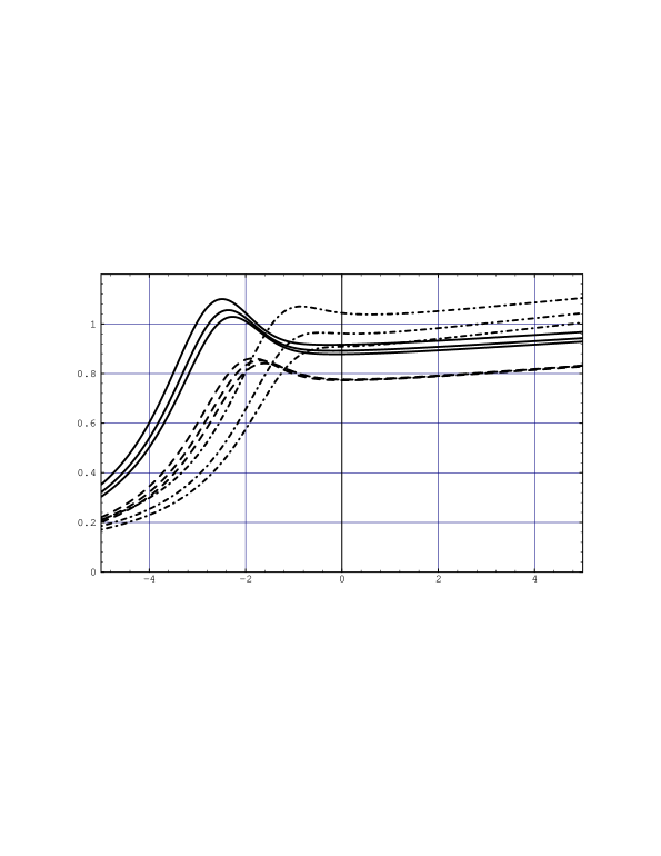
Figure 1: $R(e^{+}e^{-}\to t\bar{t})$ for the LO (dashed-dotted lines ), NLO (dashed lines), NNLO (solid lines) approximation as a function of energy $E=\sqrt{s}-2m$, GeV. In all cases we use $m_{t}=$175 GeV,$\Gamma_{t}=$1.43 GeV, $\alpha_{s}(m_{Z})=$0.118 but different values of the soft scale $\mu_{s}=50,75,100$ GeV .

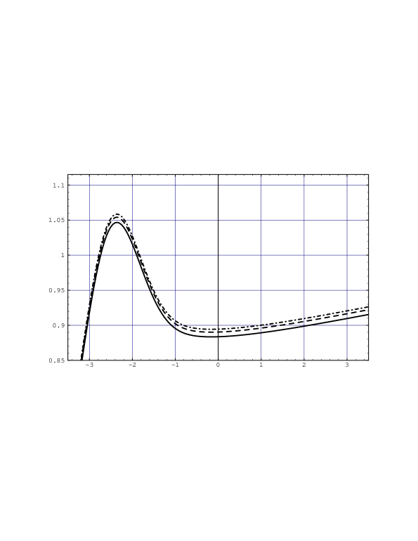
Figure 2: $R(e^{+}e^{-}\to t\bar{t})$ at NNLO at different values of factorization scale $r_{0}=2a$(dashed-dotted line), $r_{0}=a$ (dashed line) and $r_{0}=a/2$ (solid line). We use $m_{t}=$175 GeV, $\Gamma_{t}=$1.43 GeV, $\mu_{s}=75$ GeV,$\alpha_{s}(m_{Z})=$0.118.

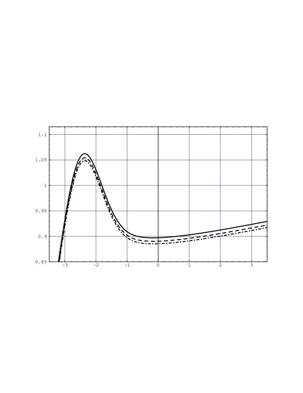
Figure 3: $R(e^{+}e^{-}\to t\bar{t})$ at NNLO at different value of the hard normalization scale $\mu_{h}=2m$(dashed-dotted line), $\mu_{h}=m$ (dashed line) and $\mu_{h}=m/2$ (solid line). We use $m_{t}=$175 GeV, $\Gamma_{t}=$1.43 GeV, $\mu_{s}=75$ GeV,$\alpha_{s}(m_{Z})=$0.118.

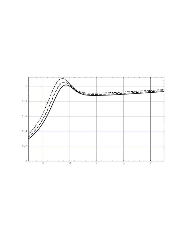
Figure 4: $R(e^{+}e^{-}\to t\bar{t})$ at NNLO at different values of the QCD coupling constant $\alpha_{s}(m_{Z})=$0.116 (solid line), $\alpha_{s}(m_{Z})=$0.118 (dashed line),$\alpha_{s}(m_{Z})=$0.120 (dashed-dotted line). We use $m_{t}=$175 GeV, $\Gamma_{t}=$1.43 GeV and $\mu_{s}=75$ GeV.

References

[1] E. Accomando et al., the ECFA/DESY LC Physics
Working Group,
Physics with linear colliders, DESY
97-100, hep-ph/9705442.
[2] V.S. Fadin and V.A. Khoze, JETP Lett. 46
(1987), 525;
Sov. J. Nucl. Phys. 48 (1988), 309.
[3] M. Peskin and M. Strassler,
Phys. Rev. D43 (1991), 1500.
[4] W. Kwong, Phys. Rev.D43 (1991), 1488.
[5] M.Jeźabek, J.H.Kühn and
T. Teubner, Z. Physik C56 (1992), 653;
Y. Sumino, K. Fujii, K. Hagiwara, H. Murayama and C.-K. Ng,
Phys. Rev. D47 (1993), 56.
[6] Y. Sumino, Ph.D thesis, Tokyo, 1993;
[7] K. Melnikov and O. Yakovlev,
Phys. Lett. B324 (1994), 217.
[8] A.H. Hoang, Phys. Rev. D56 (1997), 5851.
[9] A.H. Hoang, J. H. Kühn and T. Teubner,
Nucl. Phys. B 452 (1995) 173.
[10] A. Czarnecki and
K.Melnikov, Phys. Rev. Lett. 80 (1998) 2531.
[11] M. Beneke and V. A. Smirnov,
Nucl. Phys. B522 (1998) 321
M. Beneke, A.Signer and V.A. Smirnov, Phys. Rev. Lett. 80
(1998) 2535.
[12] A.H. Hoang and T. Teubner, preprint UCSD/PTH 98-01,
DESY 98-008, hep-ph/9801397.
[13] K. Melnikov and A. Yelkhovsky,
Nucl.Phys. B528 (1998) 59.
[20] M. Beneke, preprint CERN-TH/98-120, hep-ph/9804241.