OKHEP–98-06
ANALYTIC PERTURBATIVE APPROACH TO QCD

A technique called analytic perturbation theory, which respects the required analytic properties, consistent with causality, is applied to the definition of the running coupling in the timelike region, to the description of inclusive $\tau$-decay, to deep-inelastic scattering sum rules, and to the investigation of the renormalization scheme ambiguity. It is shown that in the region of a few GeV the results are rather different from those obtained in the ordinary perturbative description and are practically renormalization scheme independent.

1 Analytic Running Coupling Constant

The conventional renormalization-group resummation of perturbative series leads to unphysical singularities in the running coupling constant. For example, the usual QCD one-loop running coupling is 

$${\alpha^{\rm PT}(Q^{2})\over 4\pi}={1\over\beta_{0}}{1\over\ln(Q^{2}/\Lambda^{2})},$$ (1)

where $\beta_{0}=11-2n/3$, $n$ being the number of quark flavors. This evidently has a singularity (Landau pole) at $Q^{2}=\Lambda^{2}$, which is unphysical and inconsistent with the causality principle. Instead, we propose replacing perturbation theory (PT) by analytic perturbation theory (APT) $\!{}^{{\bf?},{\bf?}}$ to enforce the correct analytic properties, for example, that the running coupling be regular except for a branch cut for $-Q^{2}\geq 0$, by adopting the dispersion relation

$${\alpha^{\rm APT}(Q^{2})\over 4\pi}={1\over\pi}\int_{0}^{\infty}d\sigma{\rho(\sigma)\over\sigma+Q^{2}-i\epsilon}\,,$$ (2)

where the imaginary part is given by the perturbative result, that is

$$\rho(\sigma)={1\over 4\pi}\rm{Im}\,\alpha^{\rm PT}(-\sigma-i\epsilon)\,.$$ (3)

This leads to a consistent spacelike coupling, which in one-loop is:

$$\alpha^{\rm APT}(Q^{2})={4\pi\over\beta_{0}}\left[{1\over\ln(Q^{2}/\Lambda^{2})}+{\Lambda^{2}\over\Lambda^{2}-Q^{2}}\right]\,.$$ (4)

The second, nonperturbative term, cancels the ghost pole.

The above defines the running coupling in the spacelike region. We can also define a timelike (or $s$-channel) coupling $\alpha_{s}(s)$,$\!{}^{{\bf?}}$ which is related to the spacelike coupling through the following reciprocal relations:

$$\alpha_{s}(s) = -{1\over 2\pi i}\int_{s-i\epsilon}^{s+i\epsilon}{dz\over z}\alpha(-z)\,,$$ (5)

$$\alpha(Q^{2}) = Q^{2}\int_{0}^{\infty}{ds\over(s+Q^{2})^{2}}\alpha_{s}(s)\,,$$ (6)

where the contour in the first integral does not cross the cut on the positive real axis. In terms of the spectral function, then,

$${\alpha_{s}(s)\over 4\pi}={1\over\pi}\int_{s}^{\infty}{d\sigma\over\sigma}\rho(\sigma)\,.$$ (7)

The spectral functions in 1-, 2-, and 3-loops are shown in Fig. 1, for $n=3$.

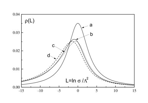
Figure 1: The spectral functions: (a) and (b) are the one- and two-loop results; (c) is the two-loop approximation obtained as the first iteration of the exact renormalization-group equation; $\!{}^{{\bf?}}$ (d) is the three-loop result in the $\overline{\rm MS}$ scheme.

The areas under all these curves turn out to be the same, which implies a universal infrared fixed point $\alpha^{*}$,

$${\alpha^{*}\over 4\pi}={\alpha(0)\over 4\pi}={\alpha_{s}(0)\over 4\pi}={1\over\pi}\int_{0}^{\infty}{d\sigma\over\sigma}\rho(\sigma)={1\over\beta_{0}}\,,$$ (8)

which is exact to all orders. $\!{}^{{\bf?},{\bf?}}$ It is also possible to prove that symmetrical behavior of the timelike and spacelike couplings is inconsistent with the required analytic properties, that is, in any renormalization scheme

$$\alpha_{s}(s)\neq\alpha(Q^{2}),\quad s=Q^{2}.$$ (9)

This difference, which is important when the value of the running coupling is extracted from various experimental data, $\!{}^{{\bf?}}$ is demonstrated in Fig. 2 for the $\overline{\rm MS}$ scheme.

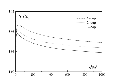
Figure 2: The ratio of spacelike and timelike values of the running coupling constant in the APT approach, at one, two, and three loops.

Because of the infrared fixed point, the running coupling implied by APT rises less rapidly for small $Q^{2}$ than does the usual perturbative running coupling. This is illustrated $\!{}^{{\bf?}}$ in Fig. 3.

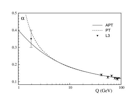
Figure 3: QCD evolution of the running coupling constants (defined in the spacelike region) compared to experimental data.$\!{}^{{\bf?}}$ Here a matching procedure across the various quark thresholds has been applied in the timelike region.$\!{}^{{\bf?}}$

Another interesting fact is that within APT Schwinger’s conjecture $\!{}^{{\bf?}}$ about the connection between the $\beta$ and spectral functions is valid.$\!{}^{{\bf?}}$ Indeed, the $\beta$ function for the timelike coupling is

$$\beta_{s}={s\over 4\pi}{d\alpha_{s}\over ds}=-{1\over\pi}\rho(s).$$ (10)

The above discussion assumes that the number of active flavors $n$ is realistically small. However, if $n$ is large enough, even the perturbative coupling can exhibit an infrared fixed point, at least in the two-loop level. This same fixed point defined by Eq. (8) occurs in the analytic approach and we have

$$\frac{\alpha^{*}}{4\pi}=\cases{1/\beta_{0}\,,&$n\leq 8\,,$\cr-\beta_{0}/\beta_{1}\,,&$9\leq n\leq 16\,.$\cr}$$ (11)

The transition between the nonperturbative and perturbative fixed point occurs for $n=8.05$, as is shown in Fig. 4. This is qualitatively consistent with the phase transition seen, for example, in nonperturbative approaches and lattice simulations.$\!{}^{{\bf?}}$

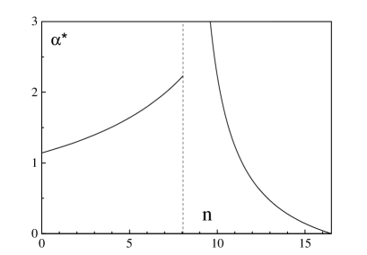
Figure 4: The analytic infrared fixed point $\alpha^{*}$ vs. $n$.

2 Inclusive $\tau$ Decay within APT

The inclusive semileptonic $\tau$ decay ratio for massless quarks is given $\!{}^{{\bf?}}$ in terms of the electroweak factor $S_{\rm EW}$, the CKM matrix elements $V_{ud}$, $V_{us}$, and the QCD correction $\Delta_{\tau}$,

$$R_{\tau}=3S_{\rm EW}(|V_{ud}|^{2}+|V_{us}|^{2})(1+\Delta_{\tau})\,.$$ (12)

The correction $\Delta_{\tau}$ may be written in terms of the functions $r(s)$ or $d(q^{2})$, which are the QCD corrections to the imaginary part of the hadronic correlator $\Pi$: ${\rm Im}\,\Pi\sim 1+r$ and to the Adler $D$-function: $D=-q^{2}d\Pi/dq^{2}\sim 1+d$. The analytic properties of the Adler function allow us to write down the relations

$$d(q^{2}) = -q^{2}\int_{0}^{\infty}{ds\over(s-q^{2})^{2}}r(s),$$ (13)

$$r(s) = -{1\over 2\pi i}\int_{s-i\epsilon}^{s+i\epsilon}{dz\over z}d(z).$$ (14)

Because of the proper analytic properties (which are violated in the usual perturbative approach) the QCD contribution to the $\tau$ ratio is given by the two equivalent forms

$$\Delta_{\tau} = 2\int_{0}^{M_{\tau}^{2}}{ds\over M_{\tau}^{2}}\left(1-{s\over M_{\tau}^{2}}\right)^{2}\left(1+2{s\over M_{\tau}^{2}}\right)r(s)$$

$$= {1\over 2\pi i}\oint_{|z|=M_{\tau}^{2}}{dz\over z}\left(1-{z\over M_{\tau}^{2}}\right)^{3}\left(1+{z\over M_{\tau}^{2}}\right)d(z).$$

If one likes, one can think of $r$ and $d$ as effective running couplings in the timelike and spacelike regions, so as with the running couplings they may be expressed in terms of an effective spectral density,

$$d^{\rm APT}(q^{2}) = {1\over\pi}\int_{0}^{\infty}{d\sigma\over\sigma-q^{2}}\rho^{\rm eff}(\sigma),$$ (16)

$$r^{\rm APT}(s) = {1\over\pi}\int_{s}^{\infty}{d\sigma\over\sigma}\rho^{\rm eff}(\sigma),$$ (17)

possessing the same universal infrared limit as the running coupling.

In the ordinary perturbative approach, the function $d(q^{2})$ may be expanded in terms of the running coupling and in the third order is

$$d^{\rm PT}(q^{2})=a^{\rm PT}(-q^{2})+d_{1}\left[a^{\rm PT}(-q^{2})\right]^{2}+d_{2}\left[a^{\rm PT}(-q^{2})\right]^{3},$$ (18)

where we have introduced $a=\alpha_{S}/\pi$, and, numerically, for three active flavors, the coefficients are $d_{1}^{\overline{\rm MS}}=1.6398$, $d_{2}^{\overline{\rm MS}}=6.3710$. Such is not the case in APT; rather, $d^{\rm APT}$ is constructed from Eq. (16) with a spectral density obtained as the imaginary part of $d^{\rm PT}$ on the physical cut:

$$\rho^{\rm eff}(\sigma)=\rho_{0}(\sigma)+d_{1}\rho_{1}(\sigma)+d_{2}\rho_{2}(\sigma),$$ (19)

where $\rho_{n}(\sigma)={\rm Im}\,a^{n+1}(-\sigma-i\epsilon)$. We use the world average $\!{}^{{\bf?}}$ value $R_{\tau}=3.633\pm 0.031$. Our results are shown in Table 1, where for the sake of illustration we also show the PT results obtained by using the contour integral representation given in the second line of Eq. (2).

Table 1: The APT and PT parameters in the $\overline{\rm MS}$ scheme extracted from $\tau$-decay. The first two rows refer to NNLO calculations, the last two rows to NLO calculations. The errors in the last digits are shown in parentheses.

Method	$\Lambda_{\overline{\rm MS}}$ (MeV)	$\alpha(M_{\tau}^{2})$	$d(M_{\tau}^{2})$
APT	871(155)	0.3962(298)	0.1446(88)
PT	385(27)	0.3371(141)	0.1339(69)
APT	918(151)	0.3983(236)	0.1431(84)
PT	458(31)	0.3544(157)	0.1400(67)

Most remarkably, APT exhibits very little renormalization scheme (RS) dependence. The $\tau$ decay coefficients $d_{1}$ and $d_{2}$ are RS dependent, as are all but the first two beta function coefficients, defined by the renormalization group equation

$$\mu^{2}{da\over d\mu^{2}}=-{b\over 2}a^{2}(1+c_{1}a+c_{2}a^{2})\,.$$ (20)

Because of the existence of RS invariants, one can investigate the sensitivity of the predicted value of the QCD correction to the choice of RS by varying $d_{1}$ and $c_{2}$ in a region where the degree of cancellation in the second RS invariant $\omega_{2}=c_{2}+d_{2}-c_{1}d_{1}-d_{1}^{2}$ does not exceed a specified limit, taking, for example,

$${|c_{2}|+|d_{2}|+c_{1}|d_{1}|+d_{1}^{2}\over|\omega_{2}|}\leq 2\,.$$ (21)

That sensitivity is shown $\!{}^{{\bf?}}$ in Fig. 5, based on $\Delta_{\tau}^{\overline{\rm MS}}=0.1881$. Observe that the relative difference between the prediction of the lower corners of the domain defined by Eq. (21) is 0.8%,

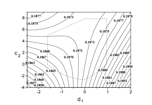
Figure 5: Contour plot of the APT correction $\Delta_{\tau}$ at the three-loop order as a function of RS parameters $d_{1}$ and $c_{2}$. The dashed line indicates the boundary of the domain defined by Eq. (21).

while in PT that difference is 5%. Note that the $\overline{\rm MS}$ scheme lies outside this domain, as does the so-called V scheme, the prediction of which differs by only 0.2% from the $\overline{\rm MS}$ value in APT, but by 66% in PT! To all intents and purposes, APT exhibits practically no RS dependence. (Because of the perturbative stability, the known three-loop level is quite adequate for these RS recalculations.)

3 Deep-Inelastic Scattering Sum Rules

At present, the polarized Bjorken and Gross–Llewellyn Smith deep inelastic scattering sum rules allow the possibility,$\!{}^{{\bf?}}$ as with $\tau$ decay, of extracting the value of $\alpha_{S}$ from experimental data at low $Q$, here down to $1\,{\mbox{\rm GeV}}$.

3.1 Bjorken Sum Rule

The Bjorken sum rule refers to the value of the integral of the difference between the polarized structure functions of the neutron and proton,

$$\Gamma_{1}^{\rm p-n} = \int_{0}^{\infty}dx\,\left[g_{1}^{p}(x,Q^{2})-g_{1}^{n}(x,Q^{2})\right]$$ (22)

$$= {1\over 6}\left|g_{A}\over g_{V}\right|\left[1-\Delta_{\rm Bj}(Q^{2})\right]\,,$$ (23)

where the prefactor in the second line is the parton-level description. In the conventional approach, with massless quarks, the QCD correction is given by a power series similar to Eq. (18), with coefficients for three active flavors being $d_{1}^{\overline{\rm MS}}=3.5833$, $d_{2}^{\overline{\rm MS}}=20.2153$. However, this description violates required analytic properties of the structure function moments, which, as has been argued,$\!{}^{{\bf?}}$ follow from the existence of the Deser-Gilbert-Sudarshan integral representation.

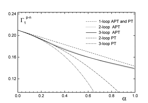
Figure 6: $\Gamma^{\rm p-n}_{1}\,$ with $1$-, $2$-, and $3$-loop QCD corrections vs. the coupling constant.

Thus we adopt the analytic approach, which says instead

$$\Delta_{\rm Bj}^{\rm APT}(Q^{2})=\delta^{(1)}(Q^{2})+d_{1}\delta^{(2)}(Q^{2})+d_{2}\delta^{(3)}(Q^{2})\,,$$ (24)

where

$$\delta^{(k)}(Q^{2})={1\over\pi^{k+1}}\int_{0}^{\infty}{d\sigma\over\sigma+Q^{2}}{\rm Im}\left[\alpha_{\rm PT}^{k}(-\sigma-i\epsilon)\right],$$ (25)

that is, $\Delta^{\rm APT}$ is not a power series in $\alpha^{\rm APT}$.

Besides possessing the correct analyticity, the APT approach has two key properties in its favor. First, successive perturbative corrections are small, so that the two- and three-loop QCD results are nearly the same. This is not the case in the conventional PT approach, as is shown $\!{}^{{\bf?}}$ in Fig. 6. Second, the renormalization scheme dependence is again very small, so that various schemes which have the same degree of cancellation as the $\overline{\rm MS}$ scheme give the same predictions all the way down to $Q^{2}\sim 1$ GeV². In contrast, it is impossible to make any reliable prediction for conventional PT, even if improved by the Padé approximant (PA) method,$\!{}^{{\bf?}}$ for $Q^{2}$ below several GeV². This is illustrated $\!{}^{{\bf?}}$ in Fig. 7. One can see that instead of RS unstable and rapidly changing PT functions, the APT predictions are slowly varying functions, which are practically RS independent.

     

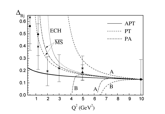
Figure 7: Renormalization scheme dependence of predictions for $\Delta_{\rm Bj}$ vs. $Q^{2}$ for the APT and PT expansions. The solid curves, which are very close to each other, correspond to the APT result in the $\overline{\rm MS}$, A, B, and ECH schemes. The PT evolution in the $\overline{\rm MS}$, A, and B schemes are shown by dashed curves, the ECH scheme is indicated by a dotted curve, and the PA results in the $\overline{\rm MS}$, A, and B schemes are denoted by dash-dotted curves. (The definition of the various schemes is given in our paper.$\!{}^{{\bf?}}$) The SMC data $\!{}^{{\bf?}}$ is indicated by a square, the triangle is the E154 data,$\!{}^{{\bf?}}$ circles are E143 data,$\!{}^{{\bf?}}$ and the stars are recent E143 data.$\!{}^{{\bf?}}$

3.2 Gross-Llewellyn Smith Sum Rule

A precisely similar analysis can be performed on the GLS sum rule, which refers to the integral

$$S_{\rm GLS} = {1\over 2}\int_{0}^{1}dx\left[F_{3}^{\overline{\nu}p}(x,Q^{2})+F_{3}^{\nu p}(x,Q^{2})\right]$$ (26)

$$= 3\left[1-\Delta_{\rm GLS}(Q^{2})\right].$$ (27)

Again, the APT approach leads to perturbative stability, and to practically no renormalization scheme dependence down to very low $Q^{2}$.$\!{}^{{\bf?}}$

4 Conclusions

Our conclusions are four-fold.

• APT maintains correct analytic properties (causality), and allows for a consistent extrapolation between timelike ($\tau$ decay) and spacelike (DIS sum rules) data.

• Three loop corrections are much smaller than in PT; thus, there is perturbative stability.

• Renormalization scheme dependence is drastically reduced. The three-loop APT level is practically RS independent.

• The values of $\Lambda$ are larger in the APT approach than in the PT approach. Yet these values are consistent between timelike and spacelike processes, and consistent with the data.

The work reported here is the beginning of a systematic attempt to improve upon the results of perturbation theory in QCD. In the future we will treat in detail the significance of power corrections which come from the operator product expansion, and examine the effect of finite mass corrections, which necessitate a more elaborate analytic structure.

References

References

- [1] D. V. Shirkov and I. L. Solovtsov, JINR Rapid Comm., No. 2 [76]-96, p. 5 (1996); Phys. Rev. Lett. 79, 1209 (1997).
- [2] K. A. Milton and I. L. Solovtsov, Phys. Rev. D 55, 5295 (1997).
- [3] K. A. Milton, I. L. Solovtsov, and O. P. Solovtsova, Phys. Lett. B 415, 104 (1997).
- [4] K. A. Milton and O. P. Solovtsova, Phys. Rev. D 57, 5402 (1998).
- [5] L3 Collaboration, M. Acciarri et al., Phys. Lett. B 404, 390 (1997); 411, 580 (1997).
- [6] J. Schwinger, Proc. Natl. Acad. Sci. USA 71, 3024, 5047 (1974).
- [7] T. Appelquist, J. Terning, and L. C. R. Wijewardhana, Phys. Rev. Lett. 77, 1214 (1996); V. A. Miransky and K. Yamawaki, Phys. Rev. D 55, 5051 (1997); J. B. Kogut and D. R. Sinclair, Nucl. Phys. B 295, 465 (1988); F. R. Brown, H. Chen, N. H. Christ, Z. Dong, R. D. Mawhinney, W. Shafer, and A. Vaccarino, Phys. Rev. D 46, 5655 (1992); Y. Iwasaki, hep-lat/9707019; Y. Iwasaki, K. Kanaya, S. Kaya, S. Sakai, and T. Toshie, hep-lat/9804005.
- [8] E. Braaten, S. Narison, and A. Pich, Nucl. Phys. B 373, 581 (1992).
- [9] Particle Data Group, R. M. Barnett et al., Phys. Rev. D 54, 1 (1996).
- [10] Particle Data Group, Eur. Phys. J. C 3, 1 1998.
- [11] K. A. Milton, I. L. Solovtsov, and V. I. Yasnov, preprint OKHEP–98–01, hep-ph/9802262.
- [12] M. Albrow et al., Proc. of Snowmass Workshop 96: New Directions for High-Energy Physics, hep-ph/9706470.
- [13] W. Wetzel, Nucl. Phys. B 139, 170 (1978).
- [14] K. A. Milton, I. L. Solovtsov, and O. P. Solovtsova, to be published in Phys. Lett. B.
- [15] S. J. Brodsky, J. Ellis, E. Gardi, M. Karliner, and M. A. Samuel, Phys. Rev. D 56, 6980 (1997), and references therein.
- [16] SMC Collaboration, A. Adams et al., Phys. Lett. B 412, 414 (1997).
- [17] E154 Collaboration, K. Abe et al., Phys. Lett. B 405, 180 (1997).
- [18] E143 Collaboration, K. Abe et al., Phys. Rev. Lett. 78, 815 (1997).
- [19] E143 Collaboration, K. Abe et al., SLAC-PUB-7753, hep-ph/9802357.
- [20] K. A. Milton, I. L. Solovtsov, and O. P. Solovtsova, in preparation.