MADPH-98-1073

FSU-HEP-980812

BNL-HET-98/27

August, 1998

QCD Corrections to Associated Higgs Boson-Heavy Quark Production

S. Dawson
Physics Department, Brookhaven National Laboratory,
Upton, NY 11973, USA

L. Reina
Physics Department, University of Wisconsin,
Madison, WI 53706, USA
and
Physics Department, Florida State University,
Tallahassee, FL 32306, USA

We compute the ${\cal O}(\alpha_{s})$ QCD corrections to the inclusive process $e^{+}e^{-}\rightarrow t\bar{t}h$. Although the total rate is small, it has a distinctive experimental signature and can potentially be used to measure the top quark-Higgs boson Yukawa coupling. The QCD corrections increase the rate by a factor of roughly $1.5$ for $e^{+}e^{-}\rightarrow t\bar{t}h$ at $\sqrt{s}\!=\!500~{}\mbox{GeV}$ and $M_{h}=100~{}\mbox{GeV}$. At $\sqrt{s}=1~{}\mbox{TeV}$, the corrections are small.

1 Introduction

The search for the Higgs boson is one of the most important objectives of present and future colliders. A Higgs boson or some object like it is needed in order to give the $W^{\pm}$ and $Z$ gauge bosons their observed masses and to cancel the divergences which arise when radiative corrections to electroweak observables are computed. We have few clues as to the expected mass of the Higgs boson, which ${\it a~{}priori}$ is a free parameter of the theory. Direct experimental searches for the Standard Model Higgs boson at LEP and LEP2 yield the limit, [1]

$$M_{h}>89.8\,\,\mbox{GeV}\,\,\,\mbox{at 95\% c.l.}$$ (1)

LEP2 will eventually extend this limit to around $M_{h}>109\,\,\mbox{GeV}\,\,\mbox{at 95\%}$ c.l. Also, from the analysis of the electroweak precision measurements an indirect upper bound can be found, [1]

$$M_{h}<280\,\,\mbox{GeV}\,\,\,\mbox{at 95\% c.l.}\,\,\,\,$$ (2)

Above the LEP2 direct search limit and below the $2Z$ boson pair production threshold is termed the intermediate mass region and is the most difficult Higgs mass region to probe experimentally. In this mass range the associated production of a Higgs boson with either a gauge boson or a fermion - antifermion pair can be an important discovery channel. In this paper, we focus on the associated production of a Higgs boson with a heavy quark pair.

The associated production of a Higgs boson with a top quark pair in $e^{+}e^{-}$ collisions has a small rate, around $1~{}fb$ for $\sqrt{s}=500~{}\mbox{GeV}$ and $M_{h}\sim 100~{}\mbox{GeV}$. However, the signature, $e^{+}e^{-}\rightarrow t{\overline{t}}h\rightarrow W^{+}W^{-}b{\overline{b}}b{\overline{b}}$, is distinctive. [2] The experimental viability of this signature has not yet been carefully evaluated.

Once the Higgs boson has been discovered, it will be important to measure its couplings to fermions and gauge bosons. These couplings are completely determined in the Standard Model with no adjustable parameters. The couplings to the gauge bosons can be measured through the associated production processes, $e^{+}e^{-}\rightarrow Zh$, $q{\overline{q}}^{\prime}\rightarrow W^{+}h$, and $q{\overline{q}}\rightarrow Zh$, and through vector boson fusion, $W^{+}W^{-}\rightarrow h$ and $ZZ\rightarrow h$. The couplings of the Higgs boson to fermions are more difficult to measure, however. [3]

The process $e^{+}e^{-}\rightarrow t{\overline{t}}h$ provides a direct mechanism for measuring the $t{\overline{t}}h$ Yukawa coupling. Since this coupling can be significantly different in a supersymmetric model from that in the Standard Model, the measurement would provide a mean of discriminating between models. The $t{\overline{t}}h$ Yukawa coupling also enters into the rates for $gg\rightarrow h$ and $h\rightarrow\gamma\gamma$, as these processes have large contributions from top quark loops. However, in these cases it is possible that there is unknown new physics which also enters into the rate and dilutes the interpretation of the signal as the measurement of the $t{\overline{t}}h$ coupling. Ref. [3] estimates that for a Higgs boson with mass less than $100~{}\mbox{GeV}$, both the $t{\overline{t}}h$ and $b{\overline{b}}h$ couplings can be measured to an accuracy of roughly $\pm 30~{}\%$ at the LHC with $600~{}fb^{-1}$ of data. It is possible that a high energy lepton collider could obtain a higher precision on the measurement of the couplings. [3]

The QCD corrections to the associated production of a Higgs boson with a heavy quark pair are the subject of this paper. They have been independently computed by Dittmaier ${\it et.al.}~{}$ [4] We compute the QCD corrections to the process $e^{+}e^{-}\rightarrow t\bar{t}h$, including only the photon exchange diagrams, which constitute the dominant contribution to the cross section. Our corrections are valid for all values of the Higgs boson mass and for any energy. Section 2 contains a review of the lowest order rate, including a discussion of the relative importance of the $Z$ boson contribution (which we neglect) and the Higgs bremsstrahlung from the $Z$ boson. The Higgs bremsstrahlung from the $Z$ is always less than a few percent effect and so the $e^{+}e^{-}\rightarrow t\bar{t}h$ process remains a candidate for measuring the coupling of the Higgs to the top quark.

The ${\cal O}(\alpha_{s})$ contributions are discussed in Sections 3 and 4. The contributions from the gluon bremsstrahlung diagrams and the separation of the calculation of the gluon emission into hard and soft pieces are presented in Section 3. The one-loop virtual contributions are discussed in Section  4. Our numerical results for $\sqrt{s}=500~{}\mbox{GeV}$ and $1~{}\mbox{TeV}$ are presented in Section 5.

The corrections to $e^{+}e^{-}\rightarrow t{\overline{t}}h$ have previously been estimated in an approximation valid at high energy and for $M_{h}<<M_{t}$. [5]. In the region where the approximation is valid, $\sqrt{s}>1~{}\mbox{TeV}$ and $M_{h}<100~{}\mbox{GeV}$, the QCD corrections were estimated to be small. We end with a comparison of our results with the approximate calculation.

2 $e^{+}e^{-}\rightarrow t{\overline{t}}h$: Lowest Order

Figure 1: Feynman diagrams contributing to the lowest order process, $e^{+}e^{-}\rightarrow t{\overline{t}}h$.

The cross section for $e^{+}e^{-}\rightarrow t\bar{t}h$ occurs through the Feynman diagrams of Fig. 1 and was first calculated in [6] (photon-exchange contribution only) and then completed in [7] (both photon and $Z$-exchange contributions). We write the cross section in the form

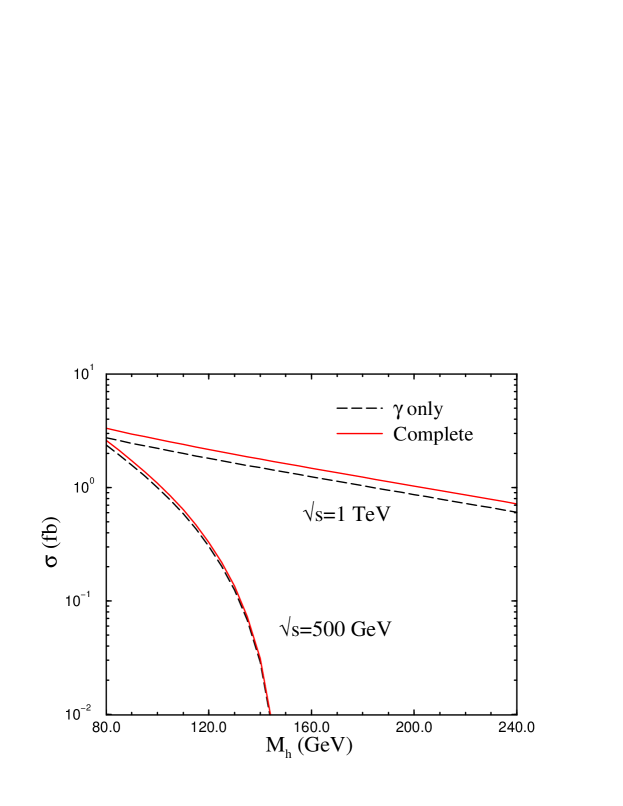
Figure 2: Lowest order cross section for $e^{+}e^{-}\rightarrow t{\overline{t}}h$ at $\sqrt{s}=500$ GeV and $\sqrt{s}=1~{}\mbox{TeV}$. The curve labelled complete includes both $\gamma$ and $Z$ exchange, along with bremsstrahlung from the $Z$ boson. We take $M_{t}=175$ GeV.

$$\frac{d\sigma(e^{+}e^{-}\rightarrow t\bar{t}h^{0})}{dx_{h}} = N_{c}\frac{\sigma_{0}}{(4\pi)^{2}}\left\{\left[Q_{e}^{2}Q_{t}^{2}+\frac{2Q_{e}Q_{t}V_{e}V_{t}}{1-M_{Z}^{2}/s}+\frac{(V_{e}^{2}+A_{e}^{2})(V_{t}^{2}+A_{t}^{2})}{(1-M_{Z}^{2}/s)^{2}}\right]G_{1}\right.$$ (3)

$$\left.+\frac{V_{e}^{2}+A_{e}^{2}}{(1-M_{Z}^{2}/s)^{2}}\left[A_{t}^{2}\sum_{i=2}^{6}G_{i}+V_{t}^{2}(G_{4}+G_{6})\right]+\frac{Q_{e}Q_{t}V_{e}V_{t}}{1-M_{Z}^{2}/s}G_{6}\right\}\,\,\,\,,$$

where $\sigma_{0}\!=\!4\pi\alpha^{2}/3s$, $\alpha$ is the QED fine structure constant, $N_{c}=3$ is the number of colors, $x_{h}=2E_{h}/\sqrt{s}$ with $E_{h}$ the Higgs boson energy, and $Q_{i}$, $V_{i}$ and $A_{i}$ ($i\!=\!e$, $t$) denote the electromagnetic and weak couplings of the electron and of the top quark respectively,

$$V_{i}=\frac{2I_{3L}^{i}-4Q_{i}s_{W}^{2}}{4s_{W}c_{W}}\,\,\,\,\,\,\,\,,\,\,\,\,\,\,\ A_{i}=\frac{2I_{3L}^{i}}{4s_{W}c_{W}}\,\,\,\,,$$ (4)

with $I_{3L}^{i}\!=\!\pm 1/2$ being the weak isospin of the left-handed fermions and $s_{W}^{2}\!=\!1-c_{W}^{2}=0.23$. (The contribution from the photon alone can be trivially found by setting $V_{i}=A_{i}=0$).

The coefficients $G_{1}$ and $G_{2}$ describe the radiation of the Higgs boson off the top quark (both photon and $Z$ boson exchange) and are given by,

$$G_{1} = \frac{2\,g_{t}^{2}}{s^{2}\left(\hat{\beta}^{2}-x_{h}^{2}\right)x_{h}}\left(\phantom{\frac{1}{2}}\!\!\!\!-4\hat{\beta}\,\left(4M_{t}^{2}-M_{h}^{2}\right)\,\left(2M_{t}^{2}+s\right)x_{h}+\right.$$

$$\!\!\!\!\!\!\!\!\!\!\!\!\!\!\!\!\!\left.\left(\hat{\beta}^{2}-x_{h}^{2}\right)\left(16M_{t}^{4}+2M_{h}^{4}-2M_{h}^{2}sx_{h}+s^{2}x_{h}^{2}-4M_{t}^{2}\left(3M_{h}^{2}-2s-2sx_{h}\right)\right)\,\log\left({\frac{x_{h}+\hat{\beta}}{x_{h}-\hat{\beta}}}\right)\right)\,\,\,,$$

$$G_{2} = \frac{-2\,g_{t}^{2}}{s^{2}\,\left(\hat{\beta}^{2}-x_{h}^{2}\right)x_{h}}\left(\phantom{\frac{1}{2}}\!\!\!\!\hat{\beta}\,x_{h}\left(-96M_{t}^{4}+24M_{t}^{2}M_{h}^{2}-\left(-M_{h}^{2}+s+sx_{h}\right)\left(-\hat{\beta}^{2}+x_{h}^{2}\right)\right)\right.+$$

$$\!\!\!\!\!\!\!\!\!\!\!\!\!\!\!\!\!\left.2\left(\hat{\beta}^{2}-x_{h}^{2}\right)\left(24M_{t}^{4}+2\left(M_{h}^{4}-M_{h}^{2}sx_{h}\right)+M_{t}^{2}\left(-14M_{h}^{2}+12sx_{h}+sx_{h}^{2}\right)\right)\log\left(\frac{x_{h}+\hat{\beta}}{x_{h}-\hat{\beta}}\right)\right)\,\,\,,$$

where $g_{t}$ is the top quark Yukawa coupling,

$$g_{t}\equiv{M_{t}\over v}\,\,\,,$$ (6)

$v=(\sqrt{2}G_{F})^{-1/2}\simeq 246~{}\mbox{GeV}$, and

$${\hat{\beta}}=\biggl{\{}{[x_{h}^{2}-(x_{h}^{min})^{2}][x_{h}^{max}-x_{h}]\over x_{h}^{max}-x_{h}+{4M_{t}^{2}\over s}}\biggr{\}}^{1/2}\,\,\,\,,$$ (7)

with $x_{h}^{min}=2M_{h}/\sqrt{s}$ and $x_{h}^{max}=1-4M_{t}^{2}/s+M_{h}^{2}/s$.

The other four coefficients, $G_{3},\ldots,G_{6}$ describe the emission of a Higgs boson from the $Z$-boson and can be written in the following form,

$$G_{3} = \frac{-2\,\hat{\beta}g_{Z}^{2}M_{t}^{2}}{M_{Z}^{2}\left(M_{h}^{2}-M_{Z}^{2}+s-sx_{h}\right)^{2}}\left(4M_{h}^{4}+12M_{Z}^{4}+2M_{Z}^{2}sx_{h}^{2}+s^{2}\left(-1+x_{h}\right)x_{h}^{2}-\right.$$

$$\left.M_{h}^{2}\left(8M_{Z}^{2}+s\left(-4+4x_{h}+x_{h}^{2}\right)\right)\right)\,\,\,,$$

$$G_{4} = \frac{\hat{\beta}g_{Z}^{2}M_{Z}^{2}}{6\left(M_{h}^{2}-M_{Z}^{2}+s-sx_{h}\right)^{2}}\left(48M_{t}^{2}+12M_{h}^{2}-s\left(-24+\hat{\beta}^{2}+24x_{h}-3x_{h}^{2}\right)\right)\,\,\,,$$ (8)

$$G_{5} = \frac{-4\,g_{t}\,g_{Z}\,M_{t}}{M_{Z}\,s\left(-M_{h}^{2}+M_{Z}^{2}+s\left(-1+x_{h}\right)\right)}\left(\phantom{\frac{1}{2}}\!\!\!\!\hat{\beta}\,s\left(6M_{Z}^{2}+x_{h}\left(-M_{h}^{2}-s+sx_{h}\right)\right)+\right.$$

$$\left.2\left(M_{h}^{2}\left(M_{h}^{2}-3M_{Z}^{2}+s-sx_{h}\right)+M_{t}^{2}\left(-4M_{h}^{2}+12M_{Z}^{2}+sx_{h}^{2}\right)\right)\,\log\left({\frac{x_{h}+\hat{\beta}}{x_{h}-\hat{\beta}}}\right)\right)\,\,\,,$$

$$G_{6} = \frac{8\,g_{t}\,g_{Z}\,M_{t}\,M_{Z}}{s\left(-M_{h}^{2}+M_{Z}^{2}+s\,\left(-1+x_{h}\right)\right)}\left(\hat{\beta}\,s+\left(4M_{t}^{2}-M_{h}^{2}+2s-sx_{h}\right)\log\left({\frac{x_{h}+\hat{\beta}}{x_{h}-\hat{\beta}}}\right)\right)\,\,\,\,,$$

where $g_{Z}$ denotes the coupling of the Higgs boson to the $Z$ boson,

$$g_{Z}\!\equiv\!{M_{Z}\over v}\,\,\,.$$ (9)

As already observed in Ref. [7], the most relevant contributions are those in which the Higgs boson is emitted from a top quark leg, i.e. those proportional to $G_{1}$ and $G_{2}$ in Eq. (3). The contribution from the Higgs boson coupling to the $Z$ boson is always less than a few per cent at $\sqrt{s}=500$ GeV and $1$ TeV and can safely be neglected. In Fig. 2, we show the complete cross section for $e^{+}e^{-}\rightarrow t{\overline{t}}h$ production and also the contribution from the photon exchange contribution only. We see that at both $\sqrt{s}=500$ GeV and $1$ TeV, the cross section is very well approximated by the photon exchange only. In the remainder of the paper, we will consider only the photon exchange contribution, neglecting the $Z$ boson exchange contribution everywhere.

3 Real Gluon Emission

Figure 3: Sample Feynman diagrams for the process $e^{+}e^{-}\rightarrow t{\overline{t}}hg$.

The ${\cal O}(\alpha_{s})$ inclusive cross section for $e^{+}e^{-}\rightarrow t{\overline{t}}h$ receives contributions from real gluon emission from the final quark legs,

$$e^{+}(p)+e^{-}(q)\rightarrow t(p_{t})+{\overline{t}}(p_{t}^{\prime})+h(p_{h})+g(k)\,\,\,\,,$$ (10)

as shown in Fig. 3. The cross section can be separated into hard and soft pieces by introducing an arbitrary separation $E_{min}$ on the gluon momenta, such that for $E_{g}<E_{min}$, we can use the eikonal approximation and calculate the cross section analytically, while for $E_{g}>E_{min}$, we integrate over the phase space numerically. The final result is of course independent of the cut-off $E_{min}$ (see Section 3.2).

3.1 Soft Gluon Radiation

For soft gluons, $E_{g}<E_{min}$, we neglect the momenta of the radiated gluons everywhere but in the singular propagators. In the soft gluon approximation, we find the contribution from the radiated gluons,

$$\biggl{(}{d\sigma\over dx_{h}}\biggr{)}_{soft}=-\biggl{(}{d\sigma\over dx_{h}}\biggr{)}_{0}\biggl{(}{g_{s}^{2}C_{F}\over(2\pi)^{3}}\biggr{)}\int_{\mid k\mid<E_{min}}{d^{3}k\over 2\omega(k)}\biggl{\{}{M_{t}^{2}\over(p_{t}\cdot k)^{2}}+{M_{t}^{2}\over(p_{t^{\prime}}\cdot k)^{2}}-{2p_{t}\cdot p_{t^{\prime}}\over(p_{t}\cdot k)(p_{t^{\prime}}\cdot k)}\biggr{\}}\,\,\,,$$ (11)

where $k$ is the gluon momentum, $\omega(k)\equiv\sqrt{\mid{\vec{k}}\mid^{2}+m_{g}^{2}}$ and we have introduced a small gluon mass $m_{g}$ to regulate the infrared divergences occurring in the soft gluon emission. The dependence on the gluon mass will be cancelled by contributions from the virtual graphs which are also evaluated with a non-zero gluon mass (see Section 4.3). The lowest order result can be found from Eq. (3).

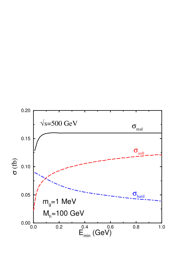
Figure 4: Contributions to the process $e^{+}e^{-}\rightarrow t{\overline{t}}hg$ as a function of the cut-off on the soft gluon energy, $E_{min}$, for fixed gluon and Higgs boson masses at $\sqrt{s}=500$ GeV. We take $M_{t}=175$ GeV and $\alpha_{s}(M_{t})=.11164$.

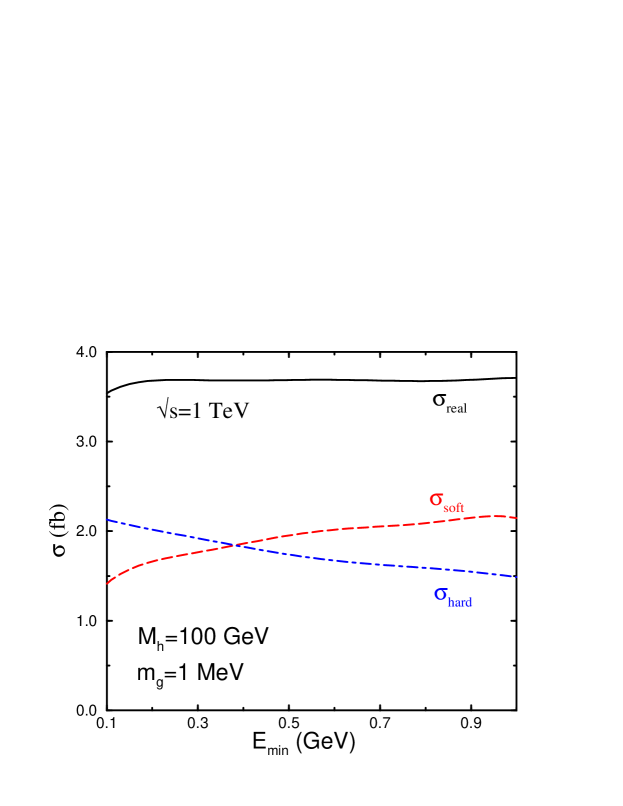
Figure 5: Contributions from the process $e^{+}e^{-}\rightarrow t{\overline{t}}hg$ as a function of the cut-off on the soft gluon energy, $E_{min}$, for fixed gluon and Higgs boson masses at $\sqrt{s}=1$ TeV. We take $M_{t}=175$ GeV and $\alpha_{s}(M_{t})=.11164$

The integral over the soft gluon phase space has been performed in Refs. [8] and [9] leading to the analytic result for the soft contribution to $e^{+}e^{-}\rightarrow t{\overline{t}}hg$,

$$\biggl{(}{d\sigma\over dx_{h}}\biggr{)}_{soft} = \biggl{(}{d\sigma\over dx_{h}}\biggr{)}_{0}{\alpha_{s}C_{F}\over 2\pi}\biggl{\{}-2\log\biggl{(}{4E_{min}^{2}\over m_{g}^{2}}\biggr{)}\biggl{[}1-{xp_{t}\cdot p_{t^{\prime}}\over M_{t}^{2}(x^{2}-1)}\log(x^{2})\biggr{]}$$ (12)

$$-{p_{t}^{0}\over\mid{\vec{p}_{t}}\mid}\log\biggl{(}{p_{t}^{0}-\mid{\vec{p}_{t}}\mid\over p_{t}^{0}+\mid{\vec{p}_{t}}\mid}\biggr{)}-{p_{t^{\prime}}^{0}\over\mid{\vec{p}_{t^{\prime}}}\mid}\log\biggl{(}{p_{t^{\prime}}^{0}-\mid{\vec{p}_{t^{\prime}}}\mid\over p_{t^{\prime}}^{0}+\mid{\vec{p}_{t^{\prime}}}\mid}\biggr{)}$$

$$+{4xp_{t}\cdot p_{t^{\prime}}\over M_{t}^{2}(x^{2}-1)}\biggl{[}{1\over 4}\log^{2}\biggl{(}{u^{0}-\mid{\vec{u}}\mid\over u^{0}+\mid{\vec{u}}\mid}\biggr{)}$$

$$+Li_{2}\biggl{(}1-{u^{0}+\mid{\vec{u}}\mid\over v}\biggr{)}+Li_{2}\biggl{(}1-{u^{0}-\mid{\vec{u}}\mid\over v}\biggr{)}\biggr{]}^{u=xp_{t}}_{u=p_{t^{\prime}}}\biggr{\}}\,\,\,,$$

where $x$ is the solution to

$$M_{t}^{2}(x^{2}+1)-2xp_{t}\cdot p_{t^{\prime}}=0\,\,\,,$$ (13)

subject to the constraint

$${xp_{t}^{0}-p_{t^{\prime}}^{0}\over p_{t^{\prime}}^{0}}>0\,\,\,,$$ (14)

and

$$v={M_{t}^{2}(x^{2}-1)\over 2(xp_{t}^{0}-p_{t^{\prime}}^{0})}\,\,\,.$$ (15)

3.2 Hard gluon radiation

The hard gluon contribution is calculated from the diagrams of Fig. 3 for gluon momenta $E_{g}>E_{min}$. The integration over the final state phase space is done using a numerical Monte Carlo. The hard gluon cross section is insensitive to the small value chosen for the gluon mass. In Figs. 4 and 5 we show the contributions of the soft and hard gluon radiation as a function of $E_{min}$. The sum of the soft and hard terms is clearly independent of the separation, $E_{min}$ for $E_{min}>>m_{g}$. The result retains a dependence on the gluon mass, $m_{g}$, however, which is cancelled when the infrared divergent pieces of the virtual contributions are included (see Section 4).

We choose $v=(\sqrt{2}G_{F})^{-1/2}\simeq 246$ GeV, $M_{t}=175$ GeV, and use the 1-loop value for $\alpha_{s}(M_{t})=.11164$ (which corresponds to $\Lambda_{QCD}=200$ MeV) in all our numerical calculations.

4 Virtual Corrections

The amplitude for $e^{+}e^{-}\rightarrow t\bar{t}h$ including virtual corrections to $O(\alpha_{s})$ can be written as

$${\cal A}={\cal A}_{0}+\frac{\alpha_{s}}{4\pi}C_{F}{\cal A}_{1}^{\rm virt}\,\,\,,$$ (16)

where $C_{F}=4/3$. We include in ${\cal A}_{1}^{\rm virt}$ also the wave function, Yukawa coupling, and mass counterterms. The corresponding contribution to the cross section at $O(\alpha_{s})$ is

$$\sigma^{\rm virt}=\frac{\alpha_{s}}{4\pi}C_{F}\,2{\rm Re}\,({\cal A}_{1}^{\rm virt}{\cal A}_{0}^{*})=\frac{\alpha_{s}}{2\pi}C_{F}{\rm Re}\,({\cal A}_{1}^{\rm virt}{\cal A}_{0}^{*})\,\,\,.$$ (17)

Figure 6: Box diagrams contributing to the virtual corrections to $e^{+}e^{-}\rightarrow t{\overline{t}}h$.

Figure 7: Vertex diagrams of type 1 contributing to the virtual corrections to $e^{+}e^{-}\rightarrow t{\overline{t}}h$.

Figure 8: Vertex diagrams of type 2 contributing to the virtual corrections to $e^{+}e^{-}\rightarrow t{\overline{t}}h$.

Figure 9: Feynman diagrams contributing to the self energy corrections of the internal heavy quark propagators for $e^{+}e^{-}\rightarrow t{\overline{t}}h$.

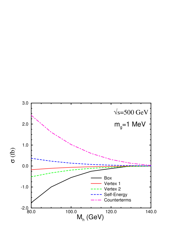
Figure 10: Contributions to $e^{+}e^{-}\rightarrow t{\overline{t}}h$ from virtual diagrams at $\sqrt{s}=500$ GeV with a finite gluon mass. We take $M_{t}=175$ GeV and $\alpha_{s}(M_{t})=.11164$

The virtual corrections we consider are:

• box diagrams (2 diagrams, see Fig. 6);

• vertex corrections of type 1 (2 diagrams, see Fig. 7 );

• vertex corrections of type 2 (2 diagrams, see Fig. 8);

• self-energy corrections to the internal leg propagators (2 diagrams, see Fig. 9);

• wave function and Yukawa coupling renormalization;

• mass renormalization (2 counterterm insertions, one for each internal propagator).

In general, virtual diagrams can have both ultraviolet (UV) and infrared (IR) singularities. In order to explicitly check the cancellation of both UV and IR divergences among different loop diagrams and counterterms, we have regularized them using dimensional regularization. We have then verified the cancellation of the $1/\epsilon_{UV}$ and $1/\epsilon_{IR}$ poles both analytically and numerically. We will discuss IR divergences in greater detail in Section 4.3.

4.1 Wave Function and Mass Renormalization Counterterms

The wave function renormalization contribution to the cross section can be expressed directly in terms of $\sigma_{0}$, the cross section at the tree level for $e^{+}e^{-}\rightarrow t{\overline{t}}h$,

$$\sigma_{Z_{2}}=\sigma_{0}^{\epsilon}\biggl{(}2\delta Z_{2}\biggr{)}\,\,\,.$$ (18)

The tree level cross section must be computed to ${\cal O}(\epsilon)$, hence we denote it by $\sigma_{0}^{\epsilon}$. We separate the infrared and ultraviolet divergences and write the wave function renormalization countertern as,

$$Z_{2} = 1+\delta Z_{2}$$

$$= 1-\frac{\alpha_{s}}{4\pi}C_{F}\biggl{(}{4\pi\mu^{2}\over M_{t}^{2}}\biggr{)}^{\epsilon}\Gamma(1+\epsilon)\left(\frac{1}{\epsilon_{UV}}+\frac{2}{\epsilon_{IR}}+4\right)\,\,\,.$$

The renormalization of the Yukawa coupling constant contributes to the ${\cal O}(\alpha_{s})$ cross section,

$$\sigma_{Y}=\sigma_{0}^{\epsilon}\biggl{(}{\delta M_{t}\over M_{t}}\biggr{)}\,\,\,,$$ (20)

where we use the pole definition of the top quark mass,

$${\delta M_{t}\over M_{t}}=-{\alpha_{s}\over 4\pi}C_{F}\biggl{(}{4\pi\mu^{2}\over M_{t}^{2}}\biggr{)}^{\epsilon}\Gamma(1+\epsilon)\biggl{(}{3\over\epsilon_{UV}}+4\biggr{)}\,\,\,.$$ (21)

Finally, there is the mass renormalization of the internal heavy quark propagators which is calculated using Eq. (21).

4.2 Calculation of Loop Diagrams

The analytical reduction of the one loop diagrams to a linear combination of one loop tensor and scalar integrals is performed using FORM, MAPLE and MAXIMA. The one loop integrals are then evaluated with the help of the numerical program FF[10]. For a fixed set of momenta, this program evaluates the finite contribution to the loop integrals numerically. The integrals over the phase space are performed with a numerical Monte Carlo. In Fig. 10, we show the finite contributions from the virtual diagrams. The virtual contribution can be written as

$$\sigma_{virt}=\sigma_{box}+\sigma_{V1}+\sigma_{V2}+\sigma_{self}+\sigma_{count}\quad,$$ (22)

where $\sigma_{box},\sigma_{V1},\sigma_{V2}$ and $\sigma_{self}$ are shown in Figs. 6 - 9. The counterterms are $\sigma_{count}=\sigma_{Z_{2}}+\sigma_{Y}+\sigma_{m}$, where $\sigma_{m}$ is the contribution of the internal propagator mass renormalization. Individually, the diagrams generate $\log(\mu^{2}/M_{t}^{2})$ contributions which are associated with $1/\epsilon_{UV}$ singularities and we take the renormalization scale $\mu=M_{t}$. Some virtual corrections also generate IR divergences and we discuss these in Section 4.3. The large cancellations between the various contributions is clear from Fig.  10.

4.3 Cancellation of Infrared Divergences

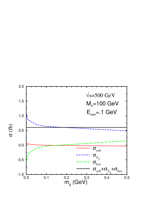
Figure 11: Contributions to $e^{+}e^{-}\rightarrow t{\overline{t}}h$ which have infrared divergences. We take $M_{t}=175$ GeV and $\alpha_{s}(M_{t})=.11164$

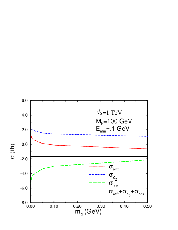
Figure 12: Contributions to $e^{+}e^{-}\rightarrow t{\overline{t}}h$ which have infrared divergences. We take $M_{t}=175$ GeV and $\alpha_{s}(M_{t})=.11164$

As we discussed before, we have verified the cancellation of the $1/\epsilon_{UV}$ ultraviolet singularities both analytically and numerically. The cancellation of the $1/\epsilon_{IR}$ singularities has also been verified analytically. Equivalently, the infrared divergences can be regulated by introducing a finite gluon mass, as was done for the real gluon diagrams of Section 3. This amounts to making the substitution

$$\Gamma(\epsilon)(4\pi\mu^{2})^{\epsilon}\rightarrow\log(m_{g}^{2})\,\,\,$$ (23)

which is what we have used in our numerical calculations.

Infrared divergences arise from the box diagram, Fig. 6, the $Z_{2}$ wavefunction renormalization, Eq. (4.1), and the soft gluon emission, Eq. (12). In Figs. 11 and 12 we show the sum of these contributions as a function of the gluon mass and see that the sum is independent of the gluon mass, confirming the cancellation of the infrared divergences.

5 Results

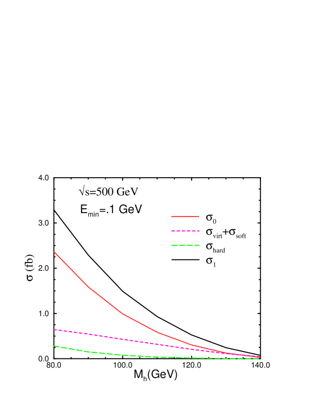
Figure 13: QCD corrections to $e^{+}e^{-}\rightarrow t{\overline{t}}h$ at $\sqrt{s}=500$ GeV. $\sigma_{0}$ is the lowest order cross section and $\sigma_{1}$ is the complete ${\cal O}(\alpha_{s})$ corrected rate. We take $M_{t}=175$ GeV and $\alpha_{s}(M_{t})=.11164$

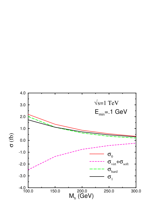
Figure 14: QCD corrections to $e^{+}e^{-}\rightarrow t{\overline{t}}h$ at $\sqrt{s}=1$ TeV. $\sigma_{0}$ is the lowest order cross section and $\sigma_{1}$ is the complete ${\cal O}(\alpha_{s})$ corrected rate. We take $M_{t}=175$ GeV and $\alpha_{s}(M_{t})=.11164$

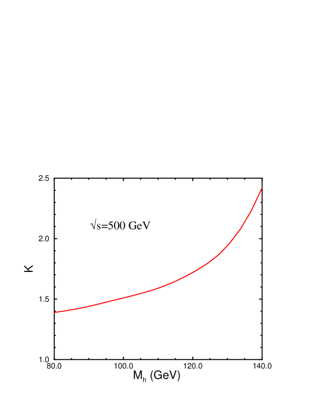
Figure 15: Ratio of the ${\cal O}(\alpha_{s})$ corrected rate to the lowest order cross section for $e^{+}e^{-}\rightarrow t{\overline{t}}h$ at $\sqrt{s}=500$ GeV. We take $M_{t}=175$ GeV and $\alpha_{s}(M_{t})=.11164$

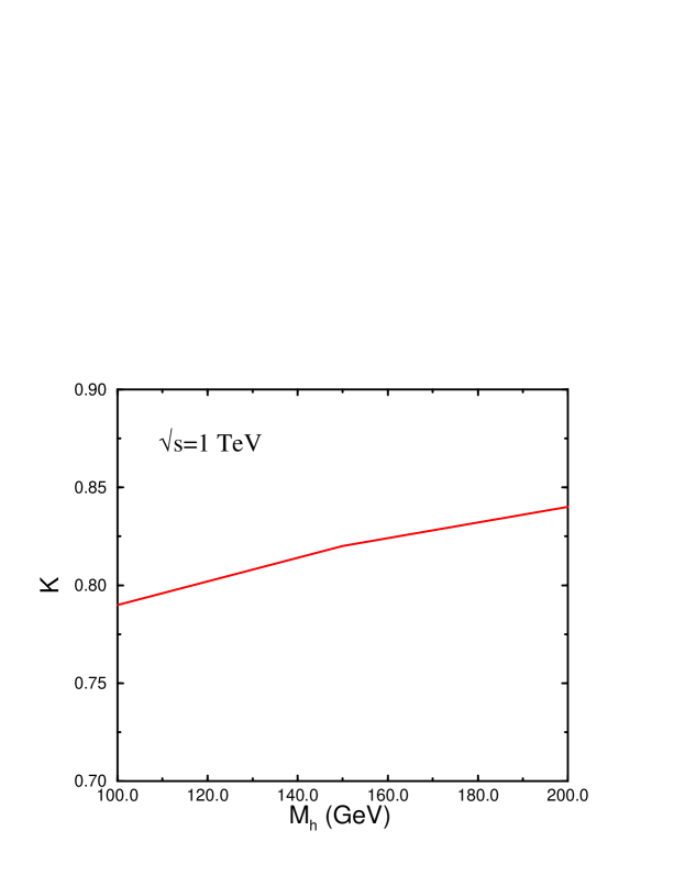
Figure 16: Ratio of the ${\cal O}(\alpha_{s})$ corrected rate to the lowest order cross section for $e^{+}e^{-}\rightarrow t{\overline{t}}h$ at $\sqrt{s}=1$ TeV. We take $M_{t}=175$ GeV and $\alpha_{s}(M_{t})=.11164$

5.1 Numerical Results

When the virtual and real contributions are combined, the final result is finite and independent of both $E_{min}$ and $m_{g}$. In Figs. 13 and 14, we show the various contributions to the total cross section. $\sigma_{1}$ is the complete ${\cal O}(\alpha_{s})$ corrected rate,

$$\sigma_{1}=\sigma_{0}+\sigma_{virt}+\sigma_{hard}+\sigma_{soft}\,\,\,.$$ (24)

The combination $\sigma_{virt}+\sigma_{soft}$ is independent of the gluon mass, but retains a dependence on $E_{min}$ which is cancelled by $\sigma_{hard}$. At $\sqrt{s}=500$ GeV, the corrections are large and positive, significantly increasing the rate. The corrections are smaller at $\sqrt{s}=1$ TeV, with large cancellations between the hard and the virtual plus soft contributions.

The size of the QCD corrections can be described by a $K$ factor,

$$K(\mu)\equiv{\sigma_{1}\over\sigma_{0}}\,\,\,,$$ (25)

which is shown in Figs.  15 and  16. Note that after the cancellation of the $1/\epsilon_{UV}$ divergences, the only $\mu$ dependence is in $\alpha_{s}(\mu)$. If $\mu=\sqrt{s}$, then $K(M_{h}=100\,\mbox{GeV})$ is reduced to $1.4$ from the value $K=1.5$ obtained with $\mu=M_{t}$ for $\sqrt{s}=500$ GeV. The authors of Ref. [4] choose $\mu=\sqrt{s}$. Our results for the $K$ factor are in agreement with theirs.

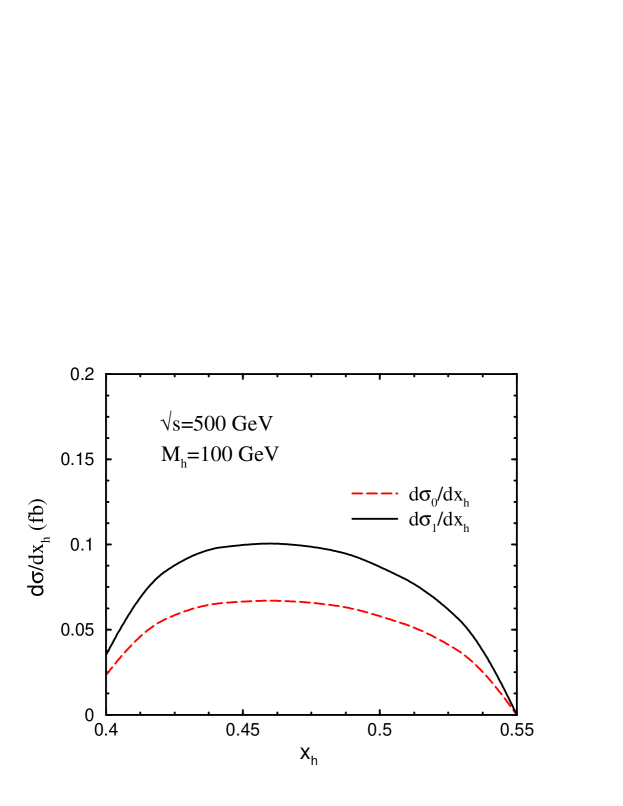
Figure 17: Differential cross section, $d\sigma/dx_{h}$, for $e^{+}e^{-}\rightarrow t{\overline{t}}h$ for $M_{h}=100$ GeV and $\sqrt{s}=500$ GeV. $\sigma_{0}$ is the lowest order cross section and $\sigma_{1}$ is the complete ${\cal O}(\alpha_{s})$ corrected rate. We take $M_{t}=175$ GeV and $\alpha_{s}(M_{t})=.11164$.

In Fig. 17, we show the shape of the differential cross section $d\sigma\over dx_{h}$ at $\sqrt{s}=500$ GeV and for $M_{h}=100$ GeV. The cross section is peaked around $x_{h}\sim.45$. Including the ${\cal O}(\alpha_{s})$ corrections has little effect on the shape of the distribution.

5.2 Comparison with Approximate Result

In Ref. [5], the ${\cal O}(\alpha_{s})$ corrections to the process $e^{+}e^{-}\rightarrow t{\overline{t}}h$ are computed in a framework where the Higgs boson is treated as a parton which is radiated from the heavy top quark. The distribution of Higgs bosons in a top quark, $f_{t\rightarrow h}(x_{h})$ is computed to ${\cal O}(\alpha_{s})$ and convoluted with the cross section for $e^{+}e^{-}\rightarrow t{\overline{t}}$, also computed to ${\cal O}(\alpha_{s})$,

$$\sigma(e^{+}e^{-}\rightarrow t{\overline{t}}h)_{EHA}=2\int^{x_{h}^{max}}_{x_{h}^{min}}dx_{h}f_{t\rightarrow h}(x_{h})\sigma(e^{+}e^{-}\rightarrow t{\overline{t}})\,\,\,.$$ (26)

This approximation, which we call the Effective Higgs Approximation (EHA), is expected to be valid for $M_{h}<<M_{t}<<\sqrt{s}$.

The impact of QCD corrections on the prediction of the cross section for $e^{+}e^{-}\rightarrow t\bar{t}h$ is described by the K-factor of Eq. (25), where the cross sections are evaluated using Eq. (26) to the appropriate order in $\alpha_{s}$. In Ref. [5], we found $K(\mu=\sqrt{s})\!\simeq.94$ at $\sqrt{s}=1$ TeV for $M_{h}\sim 100$ GeV. Comparing with Fig. 16, we see good agreement between the EHA at $\sqrt{s}=1$ TeV and the exact calculation presented here. However, the hard gluon bremsstrahlung terms of Section 3 cannot be adequately included within the context of the EHA. From Fig. 5, it is apparent that the hard gluon terms are not small. Hence the agreement between the EHA and the present calculation seems to derive from some more complicated cancellation between the hard gluon terms and those $O(M_{t}^{2}/s)$, $O(M_{h}^{2}/s)$ and $O(M_{h}^{2}/M_{t}^{2})$ contributions that are also sistematically neglected in the EHA.

6 Conclusion

We have computed the ${\cal O}(\alpha_{s})$ corrected rate for $e^{+}e^{-}\rightarrow t{\overline{t}}h$. At $\sqrt{s}=500$ GeV, the corrections are large and positive, while at $\sqrt{s}=1$ TeV, the QCD corrections are small. Studies of the experimental viability of this process as a means of measuring the top quark -Higgs boson Yukawa coupling are needed in order to assess the usefulness of the $t{\overline{t}}h$ process.

References

- [1] P. McNamara, “Standard Model Higgs at LEP”, talk presented at the International Conference for High Energy Physics, Vancouver, July 1998.
- [2] E. Accomando et.al., Phys. Rep. 299 (1998) 1.
- [3] J. Gunion et. al., New Directions in High Energy Physics, Proceedings of 1996 DPF/DPB Summer Study on High Energy Physics, (Snowmass, Colorado, 1996).
- [4] S. Dittmaier et.al., DESY 98-111.
- [5] S. Dawson and L. Reina, Phys. Rev. D57 (1998) 5851.
- [6] K.J.F. Gaemers and G.J. Gounaris, Phys. Lett. B77 (1978) 379.
- [7] A. Djouadi, J. Kalinowski and P.M. Zerwas, Zeit. Phys. C54 (1992) 255.
- [8] G. ’t Hooft and M. Veltman, Nucl. Phys. B153 (1979) 365.
- [9] A. Dennner, Fort. Phys. 41 (1993) 307.
- [10] G. van Oldenborg and J. Vermaseren, Z. Phys. C46 (1990) 425; Comp. Phys. Comm. 66 (1991) 1.
- [11] For a review and references to the literature, see M. Spira, Fortsch. Phys. 46 (1998) 203.