LU TP 98-15

hep-ph/9808436

August 1998

The Feynman–Wilson gas and the Lund model
B. Andersson, G. Gustafson, M. Ringnér and P.J. Sutton

Department of Theoretical Physics, Lund University,

Sölvegatan 14A, S-223 62 Lund, Sweden

We derive a partition function for the Lund fragmentation model and compare it with that of a classical gas. For a fixed rapidity “volume” this partition function corresponds to a multiplicity distribution which is very close to a binomial distribution. We compare our results with the multiplicity distributions obtained from the JETSET Monte Carlo for several scenarios. Firstly, for the fragmentation vertices of the Lund string. Secondly, for the final state particles both with and without decays.

1 Introduction

The cross-sections of QCD multiparticle production processes at high energies have many similarites with the multiparticle distributions of a classical gas, an analogy which was first noted by Feynman and Wilson [1]. This gas is essentially one dimensional in rapidity space. In this paper we use the gas analogy to derive a partition function for the Lund string fragmentation model [2]. We perform a virial expansion to the second order in the density of particles. Our partition function then yields an equation of state for a Van der Waal’s gas. Furthermore, it reduces to that of an ideal gas when the produced particles are massless.

The partition function of the gas is related in a simple way to the multiplicity distribution of its constituent particles. This provides us with a method of investigating the partition function. We show that for a fixed rapidity “volume” our partition function corresponds to a multiplicity distribution which is very similar to a binomial distribution.

For large rapidity intervals the major fluctuations in multiplicity stem from gluon radiation. We will, however, neglect gluon emission. In this paper we are only interested in comparing the Lund fragmentation model with the properties of a classical gas.

We analyse the multiplicity distributions obtained from the JETSET Monte Carlo [3] for several scenarios. Firstly, we investigate the string break-up vertices, then the primary particles and finally we include decays. We find that all cases are remarkably well described by distributions from the binomial family. In the derivation of our partition function we assume that the particles are ordered in rapidity. Since this is true for the vertices, we expect the distributions of vertices to be the optimal case. Indeed, these distributions are well described by our partition function.

The transition from vertices to particles introduces some smearing in rapidity. This results in a wider multiplicity distribution, where the width is sensitive to the transverse mass of the produced particles. We obtain an ordinary binomial for the primary particles. However, the strong smearing from decays ensures that, for the final state particles, this distribution becomes a negative binomial distribution.

We shall begin with a short presentation of the basic ideas of the Feynman–Wilson gas (FWG). This is followed by an introduction to the Lund model and its relationship to the FWG. We next turn to the multiplicity distributions for the vertices and lastly how they are modified for the final state particles.

2 The Feynman–Wilson gas

The original discussion of the FWG can be found in [1]. Here we summarize the main features of the model. We consider a multiparticle production process where the two primary particles have four momenta $p_{1}$ and $p_{2}$ and large invariant $s=(p_{1}+p_{2})^{2}$. The $n$ secondary particles have four momenta $k_{1},k_{2},\dots,k_{n}$, and each is on the mass shell. In the FWG model the three remaining degrees of freedom in each $k_{i}$ correspond to the “spatial” co-ordinates of a gas particle via

$$\tilde{x} = k_{x}$$

$$\tilde{y} = k_{y}$$

$$\tilde{z} = \ln[(k_{z}+k_{0})/m_{\perp}]$$ (1)

where the transverse mass is defined by

$$m_{\perp}=\sqrt{m^{2}+k_{x}^{2}+k_{y}^{2}}\;\;.$$ (2)

Note that in this picture $\tilde{z}$ corresponds to the rapidity of the relevant particle. We will assume here that each produced particle is of the same type (each has the same mass) but the extension to different species is straightforward.

We can write the total cross section for the production process using these spatial variables. We first note that the invariant phase space $d^{3}k/k_{0}$ becomes $d^{3}\tilde{r}$. The energy momentum conserving delta functions are first written in terms of $p=p_{1}+p_{2}-k_{1}-\dots-k_{n}$.

$$\delta(p_{0})\delta^{3}(p)=2\delta(p_{+})\delta(p_{-})\delta^{2}(p_{\perp})$$ (3)

with $p_{\pm}=p_{0}\pm p_{z}$. This can be expressed in terms of $\tilde{r}$ variables using the relationship $k_{0}\pm k_{z}=m_{\perp}e^{\pm\tilde{z}}$.

The delta functions have the effect of introducing a fixed volume for the gas. The transverse momenta are limited and constrain the gas to a narrow tube of radius $\sim 300$ MeV. We shall instead focus on the $\tilde{z}$ co-ordinate. We first introduce $W_{+}$ and $W_{-}$ via

$$W_{\pm}\equiv(p_{1}+p_{2})_{\pm}$$ (4)

so that we can write

$$\delta(p_{\pm})=\delta(W_{\pm}-\sum m_{\perp i}\exp(\pm\tilde{z}_{i}))\;.$$ (5)

In the following we use the Lorentz frame where $W_{\pm}=\sqrt{s}$. The two delta distributions contain the requirement that the the “gas volume” should be of the order of $\ln s$. To see this we may integrate out the rapidities of the first and the last particles to obtain

$$d\tilde{z}_{1}d\tilde{z}_{n}\,\delta(\cdots)\delta(\cdots)\simeq 1/s$$

$$\tilde{z}_{1}\simeq-\tilde{z}_{n}\;\simeq\;\ln(\sqrt{s})\;.$$ (6)

We may in this approximation choose a number $s_{0}$ in such a way that

$$\Delta\tilde{z}\equiv\tilde{z}_{1}-\tilde{z}_{n}=\ln(s/s_{0})$$ (7)

and assume that all the particles are kept inside this rapidity “volume”. If the spatial co-ordinates of the primary particles are $R_{1}$ and $R_{2}$ respectively then the cross section can be written as

$$\sigma_{T}(R_{1},R_{2})=\sum_{n=2}^{\infty}\left[\left(\prod_{i}^{n}\int d^{3}\tilde{r}_{i}\right)\;2\delta(p_{+})\delta(p_{-})\delta^{2}(p_{\perp})\;\sigma_{n}(\tilde{r}_{1},\dots,\tilde{r}_{n},R_{1},R_{2})\right]\;.$$ (8)

For fixed $R_{1},R_{2}$ then $\sigma_{T}$ corresponds, in the FWG analogy, to the partition function of the gas and the functions $\sigma_{n}$ are the $n$ particle distribution functions for the gas. Our aim is to connect these ideas to particle production within QCD as represented by the Lund model.

3 The Lund model and the Feynman–Wilson gas

3.1 The Lund model

In this section we briefly review some features of the Lund model fragmentation scheme. We will mostly be concerned with the simple situation when the colour force field from an original quark-antiquark pair (produced by $\mbox{e}^{+}\mbox{e}^{-}$ annihilation, for example) decays into a set of final state hadrons.

In the Lund model, the colour force field is approximated by a massless relativistic string with a quark (q) and an antiquark ($\overline{\mbox{q}}$) at the endpoints. The gluons are treated as internal excitations on the string field. This means that there is a constant force field, $\kappa\simeq 1~{}\mbox{GeV}/\mbox{fm}$, corresponding to a linearly rising potential, spanned between the original pair. After being produced the q and the $\overline{\mbox{q}}$ are moving apart and the energy in the field can be used to produce new $\mbox{q}\overline{\mbox{q}}$-pairs. When a new pair is created the string is split into two pieces.

The production rate of a pair with combined internal quantum numbers corresponding to the vacuum is, from quantum mechanical tunneling in a constant force field, given by

$$P(\mu_{\perp})=\exp\left(-\frac{\pi\mu_{\perp}^{2}}{\kappa}\right).$$ (9)

Here the quarks in the pair have transverse mass $\mu_{\perp}=\sqrt{\mu^{2}+\vec{k}_{\perp}^{2}}$, mass $\mu$ and transverse momentum $\pm\vec{k}_{\perp}$. The final state mesons in the Lund model correspond to isolated string pieces containing a q from one breakup vertex and a $\overline{\mbox{q}}$ from the adjacent vertex together with the produced transverse momentum and the field energy in between. The break-up of the string is illustrated in Fig.(1).

One necessary requirement is that to obtain real positive (transverse) masses all the vertices must have spacelike difference vectors. Together with Lorentz invariance this means that all the vertices in the production process must be treated in the same way [4]. Another consequence is that it is always the slowest mesons that are produced first in any Lorentz frame (corresponding to the fact that time-ordering is frame dependent). Furthermore each vertex has the property that it will divide the event into two causally disconnected jets, the mesons produced along the string field to the right and those produced to the left of the vertex. This can be seen in Fig.(1).

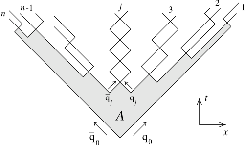
Figure 1: The break-up in space–time of a Lund string into $n$ hadrons. The fragmentation area is denoted by $A$.

A convenient ordering along the force field of the produced particles is rank ordering. Two particles have adjacent rank if they share a $\mbox{q}\overline{\mbox{q}}$ pair created at a vertex . The first rank meson contains the internal quantum numbers of the original q together with those of the $\overline{\mbox{q}}$ produced at the vertex closest to the endpoint q. Similarly the second rank meson contains the internal quantum numbers of the q from this “first” vertex and the $\overline{\mbox{q}}$ of the “second” etc. In this way rank ordering corresponds to an ordering along a light-cone. Alternatively it is also possible to rank order in the direction from the original $\overline{\mbox{q}}$.

The basic Lund model fragmentation process then stems from the following two assumptions

1. In the centre of phase space (i.e. far from the endpoints) the string decay process will reach a steady state. The probability to find a vertex is, after many production steps along the light-cone, a finite distribution in the proper time of the vertex. This is also the case when the total string field energy becomes very large.

2. The decay process is the same whether it is ordered along the positive or along the negative light-cone.

Figure 2: The production, in energy–momentum space, of a particle with transverse mass $m_{\perp}$. The particle is produced between the vertices 1, with the squared proper-time $\tau_{1}^{2}=\Gamma_{1}/\kappa^{2}$, and 2, with $\tau_{2}^{2}=\Gamma_{2}/\kappa^{2}$. The particle has fractional light-cone components $z_{+}$ and $z_{-}$.

If we consider Fig.(2), this means that we assume that the probability to reach the space-time point 1 at $(x_{+1},x_{-1})$, after many steps along the positive light-cone, and to produce a meson with transverse mass $m_{\perp}$ by one further step to the vertex 2 at $(x_{+2},x_{-2})$, is equal to the probability to reach the point 2, after many steps along the negative light-cone, and by one further step to 1 produce the meson with $m_{\perp}$.

Changing variables to the squared Lorenz invariant proper time $\tau^{2}=x_{+}x_{-}$ and the rapidity $y=1/2\ln{(x_{+}/x_{-})}$ the probability to reach the point 1 is $H(\tau_{1}^{2})d\tau_{1}^{2}dy_{1}$. The probability to produce one further particle with mass $m_{\perp}$ and fractional light-cone component $z_{+}$ is $f(z_{+},m_{\perp})dz_{+}$. A particle with fractional light-cone component $z_{+}$ has the positive light-cone energy-momentum component $p_{+}=z_{+}\kappa x_{+1}$ and has, in order to stay on the mass-shell, the negative component $p_{-}=m_{\perp}^{2}/p_{+}=z_{-}\kappa x_{-2}$. This means that we obtain the equation:

$$H(\tau_{1}^{2})d\tau_{1}^{2}f(z_{+},m_{\perp})dz_{+}=H(\tau_{2}^{2})d\tau_{2}^{2}f(z_{-},m_{\perp})dz_{-}\;.$$ (10)

It is a nice and surprising feature of the assumptions above that there is a unique process that fulfills Eq.(10) [4],

$$H_{j} = C_{j}\Gamma^{a_{j}}\exp(-b\Gamma)~{}~{}~{}~{}\mbox{with}~{}~{}\Gamma=\kappa^{2}\tau^{2}\;,$$

$$f_{jk} = \hat{N}_{jk}z^{a_{j}-1}\left(\frac{1-z}{z}\right)^{a_{k}}\exp(-bm_{\perp}^{2}/z)\;.$$ (11)

The numbers $C_{j}$ and $\hat{N}_{jk}$ are normalisation constants and the particle is assumed to be produced in a step from a vertex with flavour $j$ to a vertex with flavour $k$. If $n_{f}$ denotes the number of $\mbox{q}\overline{\mbox{q}}$-flavours, the process has $n_{f}+1$ parameters. Although the parameter $a$ is, in principle, flavour dependent, there has been no need to utilize this in the Lund model as implemented in the JETSET Monte Carlo; except for the first rank particle in a heavy quark jet [5]. The parameter $b$ must be flavour independent.

It is possible to construct the probability to produce a finite energy cluster of rank-connected particles [4] from Eq.(3.1). Such a cluster is shown in Fig.(3).

Figure 3: The decay, in energy-momentum space, of an $n$-particle cluster with invariant squared mass $s$. The fragmentation area of the cluster is $A_{\mbox{\scriptsize rest}}$. $\Gamma=\kappa^{2}\tau^{2}$ is with respect to the proper-time $\tau$ of the last vertex.

This probability distribution is in a natural way subdivided into two parts, the probability to obtain the cluster and the probability that the cluster decays in a particular way. In the following we order the particles along the positive light-cone. If the cluster has a total light-cone fraction $z$ and a fixed total squared cms energy $s$ then the (non-normalised) probability to obtain such a cluster is

$$dP_{\mbox{\scriptsize ext}}=\frac{dz}{z}z^{a_{0}}\left(\frac{1-z}{z}\right)^{a_{n}}\exp(-b\Gamma(s,z))~{}~{}~{}~{}\mbox{with}~{}~{}\Gamma(s,z)=s\frac{1-z}{z}\;.$$ (12)

The cluster then starts at a vertex with flavour $f_{0}$ and ends with flavour $f_{n}$. The $\Gamma$ value is that of the last vertex, as shown in Fig.(3). Thus a cluster is produced in the same way as a single particle between the vertices with $a_{0}$ and $a_{n}$. Similarly we find that the (non-normalised) probability for the cluster to decay into the particular channel with the particles $\{p\}_{j}$ is

$$dP_{\mbox{\scriptsize int}}=\left[\prod\hat{N}_{j}dp_{j}\delta(p_{j}^{2}-m_{j}^{2})\right]\delta(\sum p_{j}-P_{\mbox{\scriptsize tot}})\exp(-bA_{\mbox{\scriptsize rest}})$$ (13)

where $A_{\mbox{\scriptsize rest}}$ is the decay area of the cluster, as shown in Fig.(3). Equation (13) is for simplicity written in the ordinary Lund model fashion with a single $a$-parameter (this parameter is not explicit in the formula) and we note the appearance of the phase space for the final state particles multiplied by the exponential area decay law. The quantity $P_{\mbox{\scriptsize tot}}$ is the total energy momentum of the cluster so that $P_{\mbox{\scriptsize tot}}^{2}=s$. We may determine the finite energy version of the vertex distribution, $H(\Gamma)$, from Eq.(12) by exchanging $z$ for $\Gamma$. This yields

$$H_{s}\propto\frac{\Gamma^{a_{n}}s^{a_{0}-a_{n}}}{(\Gamma+s)^{a_{0}+1}}\exp(-b\Gamma)\;.$$ (14)

The function $H_{s}$ in Eq.(14) is exponentially decreasing in $\Gamma$ so that the power dependence in the denominator only plays a role for small values of $\Gamma$ and then it is hardly noticable for large values of $s$. In this way the assumption $1.$ above is fulfilled. That is to say when $s$ becomes very large there is (after normalisation) a finite distribution in the proper-time size of the decay vertices.

3.2 The connection between the Lund model and the FWG

We will now exhibit the decay distribution of a cluster, as given by Eq.(13), in terms of the partition function which is studied in statistical physics. For simplicity we write the formulas for a single particle transverse mass $m_{\perp}$ and a single flavour and we let $j$ denote the rank of a particle. The phase space factor can in analogy with the result in section 2 be written with the particle energy momentum vectors $p_{j}\equiv m_{\perp}(\exp(y_{j}),\exp(-y_{j}))$ as

$$d\Psi \equiv \left[\prod\hat{N}dp_{j}\delta(p_{j}^{2}-m_{j}^{2})\right]\delta(\sum p_{j}-P_{tot})$$ (15)

$$= \left[\prod_{1}^{n}\hat{N}dy_{j}\right]\delta(\sum m_{\perp}\exp(y_{j})-P_{+})\delta(\sum m_{\perp}\exp(-y_{j})-P_{-})$$

$$\simeq \frac{\hat{N}^{2}}{s}\prod_{2}^{n-1}\hat{N}dy_{j}\;.$$

We have in the last line integrated out the first and the last rapidities in the delta function and from now on we assume that the remaining particles are placed in rapidities between $\Delta y/2$ and $-\Delta y/2$ with $\Delta y=\ln(s/s_{0})$ and $s_{0}$ is some suitable scale. If all the particles are ordered in rapidity we may integrate out the phase space factor and obtain

$$\int d\Psi=\frac{\hat{N}^{2}(\hat{N}\Delta y)^{n-2}}{s(n-2)!}\;.$$ (16)

We next consider the decay area of the cluster. Figure (4) shows that it can be written in terms of the rapidities of the particles

$$A=m_{\perp}^{2}\sum_{j=1}^{n}\sum_{k=j}^{n}\exp(y_{k}-y_{j})\;.$$ (17)

From this equation and Eq.(15) we note that the decay distribution in Eq.(13) has similarities with a partition function, $Z_{n}$, and we therefore define a grand partition function $Z$ as

$$Z=\sum_{n}Z_{n} = s\;\sum_{n}\left[\left(\prod_{j=1}^{n}\hat{N}dy_{j}\right)\delta(\ldots)\delta(\ldots)\exp\left(-bm_{\perp}^{2}\sum_{j=1}^{n}\sum_{k=j}^{n}\exp(y_{k}-y_{j})\right)\right]$$ (18)

$$\equiv s\;\sum_{n}\left[\left(\prod_{j=1}^{n}\hat{N}dy_{j}\right)\delta(\ldots)\delta(\ldots)\exp\left(-\frac{1}{kT}\sum_{j=1}^{n}\sum_{k=j}^{n}V(y_{j}-y_{k})\right)\right]\;.$$

(The factor of $s$ is required in order to have a dimensionless partition function.) In this way we see that the decay distribution in Eq.(13) may be interpreted as the partition function for a system of $n$ particles with co-ordinates $y_{j}$ interacting with exponential two-body potentials in a one-dimensional volume equal to $\Delta y$. We note that whilst all the particles interact in this way (“long-range interactions”) the exponential decrease of the potentials ensures that the effective interaction is rather short ranged.

Figure 4: The fragmentation area partitioned into two-particle regions reveals how the area can be expressed as in Eq.(17).

If the particles are imagined as making up a gas in rapidity space and are interacting via two-body potentials, then the Hamiltonian is

$$H=\sum_{j}T(\pi_{j})+\sum_{j,k}V(y_{j}-y_{k})\;.$$ (19)

The phase space volume element is $\prod(dy_{j}d\pi_{j})$, with $\pi_{j}$ denoting the quantities canonically conjugate to the co-ordinates $y_{j}$. The kinetic energy factors $T$ are integrated out in Eq.(18) and incorporated into the constants $\hat{N}$. These constants then play the role of fugacities.

We shall now attempt to obtain a simplifed expression for the partition function, $Z_{n}$. We have already seen that in the strong ordering limit the phase space may be easily integrated according to Eq.(16). Using this limit may seem drastic since two neighbours in rank may well have a different rapidity order. However, if many pairs are not well ordered then many of the exponential potentials in the in the partition function will be strongly increasing, i.e. the area suppression in the Lund model will make these contributions small.

We can easily find an expression for the exponential in our partition function if we approximate the fragmentation area. Assuming that each particle lies along the hyperbola with $<\sqrt{\Gamma}>=\gamma$ then each takes up a rapidity length $\delta=m_{\perp}/\gamma$. Consequently all the $n$ particles take up the rapidity length $\Delta y=n\delta=nm_{\perp}/\gamma$ and the total area is $\gamma^{2}\Delta y=n^{2}m_{\perp}^{2}/\Delta y$. Since the particles are produced around the average hyperbola, we expect that this result may be modified by a constant, $c_{2}$, of order unity giving

$$bA\simeq\frac{bc_{2}m_{\perp}^{2}n^{2}}{\Delta y}=\frac{c_{3}n^{2}}{\Delta y}\;,$$ (20)

where we have introduced $c_{3}=bm_{\perp}^{2}c_{2}$. In this way we obtain from Eq.(16) and Eq.(20) a description of the grand partition function in terms of the multiplicity $n$. In the approximation that $n$ is large, i.e. for large rapidity intervals $\Delta y$, we can write the partition function in terms of two parameters $c_{1}$ and $c_{3}$ as

$$Z_{n}\simeq\frac{(c_{1}\Delta y)^{n}}{n!}\exp\left(\frac{-c_{3}n^{2}}{\Delta y}\right)\;.$$ (21)

We will comment further on the parameters $c_{1}$ and $c_{3}$ when we investigate to what extent the partition function in Eq.(21) describes the particle production in the Lund model.

3.3 The partition function in the Gaussian approximation

We now investigate the grand partition function in the limit where the number of particles is large, but the density is low (as in an ordinary gas). In this case we expect that the grand partition function can be approximated by the maximal term in the sum. To find the multiplicity for which the partition function is maximal we first define $\Phi_{n}$ by writing Eq.(21) as

$$Z_{n}=\exp\Phi_{n}\;.$$ (22)

If we treat $n$ as a continuous variable we can expand $\Phi_{n}$ in a Taylor series as

$$\Phi(n)\simeq\Phi({\overline{n}})+(n-\overline{n})\;\Phi^{\prime}({\overline{n}})+\frac{(n-\overline{n})^{2}}{2}\;\Phi^{\prime\prime}({\overline{n}})\;.$$ (23)

Choosing ${\overline{n}}$ such that $\Phi^{\prime}({\overline{n}})=0$, we evidently have a Gaussian approximation for $Z_{n}$

$$Z_{n}\simeq\exp\Phi({\overline{n}})\;\exp\left(-\frac{(n-{\overline{n}})^{2}}{2V}\right)$$ (24)

where the variance, $V$, is given by $V=1/\Phi^{\prime\prime}({\overline{n}})$. It is straightforward to obtain expressions for both ${\overline{n}}$ and $V$ if we use Stirlings approximation for the factorial in $\Phi(n)$. We find

$${\overline{n}} = \frac{\Delta y}{2c_{3}}\;\ln(\frac{c_{1}\Delta y}{\overline{n}})$$

$$V = {\overline{n}}\left(1+\frac{2c_{3}{\overline{n}}}{\Delta y}\right)^{-1}\;.$$ (25)

Notice that, since $c_{3}$ is positive, this implies that the variance of the distribution is less than the mean and the distribution is therefore narrower than a Poissonian. If we now introduce the density of particles in the rapidity volume, $R=\overline{n}/\Delta y$, then

$$\Phi({\overline{n}})=(R+c_{3}R^{2})\Delta y\;.$$ (26)

For large ${\overline{n}}$ we can approximate the grand partition function as $Z\sim Z_{\overline{n}}$ and so

$$Z\sim\left(\frac{s}{s_{0}}\right)^{a_{R}}$$ (27)

with

$$a_{R}={R+c_{3}R^{2}}\;.$$ (28)

The grand canonical partition function, for a gas is related to the pressure, $P$, temperature, $T$ and volume, $\ln(s/s_{0})$, of the gas via

$$\Omega \equiv -kT\ln Z$$

$$P = -\frac{\partial\Omega}{\partial\ln(s/s_{0})}$$ (29)

where $k$ is Boltzmann’s constant. For the partition function in Eq.(27) we obtain the following equation of state for the gas

$$P=kT(R+c_{3}R^{2})\;.$$ (30)

Our expansion thus corresponds to the first two terms in the virial expansion in the particle density of the gas. We note that the equation of state in Eq.(30) is similar to that of a Van der Waal’s gas. For particles with zero (transverse) mass we have $c_{3}=0$. In this case a particle does not take up any volume in rapidity and Eq.(30) reduces to the equation of state for an ideal gas.

4 The vertex distributions

The partition function is related to the multiplicity distribution, $P_{n}$, since

$$P_{n}\;=\frac{Z_{n}}{Z}\;\;.$$ (31)

In the remaining sections we shall use this relationship to further study our partition function. We begin here with a study of the vertices produced in the string fragmentation. These vertices are strongly ordered in rapidity and thus satisfy one of the assumptions used to derive our partition function. This is only an approximation in the case of the particles. Of course, the number of vertices corresponds directly to the number of primary particles.

In what follows we outline a simple model in which all particles have the same mass ($m=0.8$ GeV) and there is no transverse momenta. The effects of relaxing those constraints will be considered in the next section where we return to the particles.

4.1 The distribution in rapidity

We begin by studying the separation between neighbouring vertices. In the Lund model the distribution of such separations for a fixed mass, $m$, is given by

$$P(\delta y)=N\int d\Gamma\;\Gamma^{a}e^{-b\Gamma}\;\int_{0}^{1}dz\;\;\frac{(1-z)^{a}}{z}\;e^{-bm^{2}/z}\;\delta\left(\delta y-\frac{1}{2}\ln\left(\frac{\Gamma+m^{2}/z}{\Gamma(1-z)}\right)\right)\;.$$ (32)

The logarithm of this distribution is plotted in Fig.(5) for various values of the Lund model parameters $a$ and $b$.

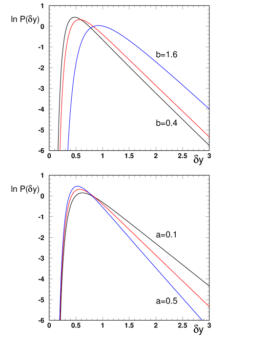
Figure 5: The logarithm of the distribution of the rapidity distance $P(\delta y)$ between adjacent vertices as predicted by the Lund model (Eq.(32)) for a fixed mass, $m=0.8$ GeV, but different values of the Lund model parameters $a$ and $b$. The upper plot shows fixed $a=0.3$ and $b=0.4$, 0.58, 1.6. The lower plot shows fixed $b=0.58$ and $a=0.1$, 0.3, 0.5.

We see from this figure that there are two main characteristics of the distribution. The first is an effective minimum separation between vertices which increases with $bm^{2}$, but is independent of $a$. Physically this separation arises because two vertices cannot be very close together in rapidity if they must produce a massive particle. The second characteristic is an exponential fall off for large separations, $\delta y$, which depends only on the parameter $a$.

We can consider a simple model which reproduces the above features very well. In this model the rapidity region is divided up into a series of $N$ equal bins of size $\delta y_{\mbox{\scriptsize bin}}$. The effective minimum separation between vertices can now be taken into account by demanding that no bin may contain more than a single vertex. Each bin is assigned a probability $p$ to contain a vertex and a probability $1-p$ to be empty. This allows us to compute the probability of a separation, $\delta y$, between two vertices. If $\delta y$ is discretised as $\delta y=n\delta y_{\mbox{\scriptsize bin}}$ with $n$ an integer then the probability of such a separation is given by a geometric series

$$P(\delta y) = p(1-p)^{n-1}~{}~{}~{}~{}~{}~{}~{}~{}~{}~{}~{}~{}~{}~{}~{}(n=1,2,\dots)$$ (33)

$$= \frac{p}{(1-p)}\exp(-\beta\delta y)$$

with $\beta=-\ln(1-p)/\delta y_{\mbox{\scriptsize bin}}$. We see that large $\delta y$ separations are exponentially suppressed. The two main features of Fig.(5) are thus very well reproduced by this simple model, which corresponds to distributing the vertices according to a binomial distribution (appendix A).

We can investigate the accuracy of the binomial approximation using the JETSET Monte Carlo (for consistency we use a fixed mass ($m=0.8$ GeV) and have no transverse momentum generation). Here we generate 2-jet ($\mbox{q}\overline{\mbox{q}}$) events and analyse the distribution of vertices within a rapidity range, $\Delta y$. The energy is chosen to be sufficiently large in order to avoid edge effects from the q and $\overline{\mbox{q}}$ fragmentation contaminating the $\Delta y$ region. The mean, $\langle n\rangle$, and the variance, $V$, of the resulting multiplicity distributions are used to calculate the binomial parameters $N$ and $p$, as detailed in appendix A. We will see later that binomial distributions with these $N$ and $p$ values do indeed reproduce the multiplicity distributions very well. Figure (6) shows the results as a function of $\Delta y$, for various values of the parameter $b$. We see that for large rapidity volumes ($\Delta y\gtrsim 5$ units) the binomial assumptions seem to work very well. That is to say, the observed $p$ parameter is effectively constant as a function of $\Delta y$, whilst the parameter $N$ is linear with $\Delta y$. This corresponds to a constant bin size $\delta y_{\mbox{\scriptsize bin}}$. (As expected the bin size is found to be proportional to $bm^{2}$.)

The behaviour of the effective JETSET $N$ and $p$ parameters at small values of $\Delta y$ can easily be understood. When $\Delta y$ becomes smaller than the normal bin size, $\delta y_{\mbox{\scriptsize bin}}$, we have only one bin which is now of size $\Delta y$. In Fig.(6) all of the $N$ curves indeed tend to the limit $N=1$. Meanwhile the observed $p$ value is the probability to find a vertex in this single bin

$$p_{\mbox{\scriptsize obs}}=p\;\frac{\Delta y}{\delta y_{\mbox{\scriptsize bin}}}\;\;\;\;\;(\Delta y<\delta y_{\mbox{\scriptsize bin}})\;\;.$$ (34)

Thus the observed $p$ becomes linear with $\Delta y$ when $\Delta y$ is smaller than the bin size. This effect can be seen in Fig.(6). Between the limits of large and small $\Delta y$ the behaviour of $N$ and $p$ are not so well determined. Here correlations between closely spaced vertices will play a role.

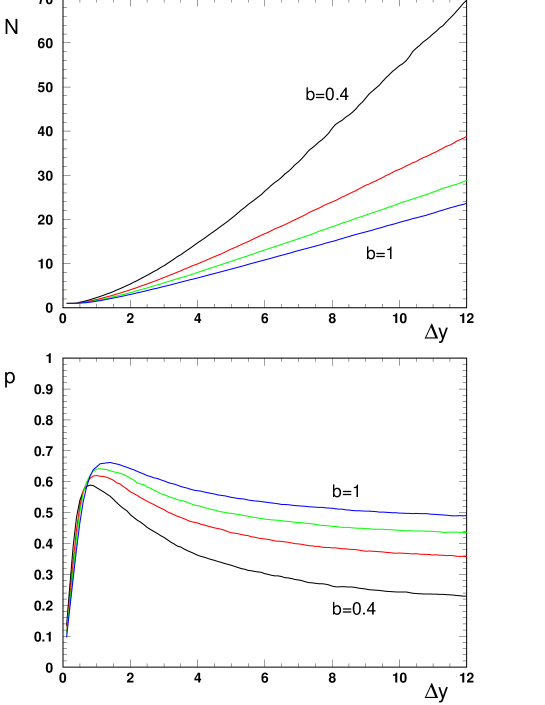
Figure 6: The values of $N$ (upper plot) and $p$ (lower plot) for the vertex distributions produced by JETSET (for a fixed mass and no transverse momentum generation) as a function of the rapidity volume, $\Delta y$. We show the results for fixed $a=0.3$ and $b=0.4$, 0.6, 0.8 and 1.

We are now in a position to turn our attention back to the partition function. This formula should also generate a good description of the multiplicity distribution for the vertices. We have

$$P_{n}\;=\;c_{0}\;\frac{(c_{1}\Delta y)^{n}}{n!}\exp\left(\frac{-bm^{2}\;c_{2}n^{2}}{\Delta y}\right)$$ (35)

Here $c_{0}$ is a normalisation parameter and so is determined in terms of the remaining parameters. We can relate the parameters $c_{1}$ and $c_{2}$ to the parameters $N$ and $p$ of the binomial distribution. The procedure is explained in detail in appendix B. For large $\Delta y$, we obtain

$$c_{1} = \frac{Np}{\Delta y}\;\exp\left[\frac{p}{(1-p)}\right]$$

$$c_{2} = \frac{\Delta y}{2bm^{2}N(1-p)}$$ (36)

In Fig.(7) we show the values of $c_{1}$ and $c_{2}$ which we obtain from our JETSET multiplicity distributions. For large rapidity volumes, $\Delta y$, they tend to constant values. We noted in section 3.3 that it is also possible to approximate Eq.(35) using a Gaussian distribution (with the appropriate mean and variance). If we express the mean and variance of Eq.(25) in terms of $N$ and $p$ and solve for $c_{1}$ and $c_{2}$, then we obtain the same expressions as Eq.(36). We note, however, that in the case of a Gaussian distribution one has a symmetric distribution. This is not true of either Eq.(35) or the binomial distribution since they both contain a term $n!$ in the denominator.

Finally in Fig.(8) we demonstrate how well the binomial and Eq.(35) reproduce the observed multiplicity distribution. We show three curves firstly the JETSET multiplicity distribution, secondly that obtained from the binomial distribution and finally the distribution obtained from Eq.(35). At $\Delta y=5$ we see very good agreement and it is difficult to distinguish the different curves whilst at $\Delta y=10$ all of the curves lie on top of each other. We thus see that the vertex multiplicity distributions produced by JETSET do indeed agree very well with our simple expression for the partition function, $Z_{n}$.

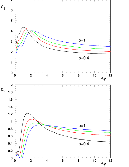
Figure 7: The values of $c_{1}$ (upper plot) and $c_{2}$ (lower plot) for the vertex distributions produced by JETSET (for a fixed mass and no transverse momentum generation) as a function of the rapidity volume, $\Delta y$. We show the results for fixed $a=0.3$ and $b=0.4$, 0.6, 0.8 and 1.

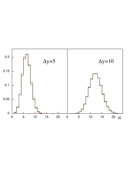
Figure 8: The multiplicity distributions for the vertices for various values of the rapidity volume $\Delta y$ as obtained from JETSET (solid curve), the binomial distribution (medium grey curve) and Eq.(35) (light grey curve).

4.2 Distribution in proper time

So far we have discussed the distribution of the vertices in terms of the rapidity, $y$. If $p_{T}$ is neglected then the position of the vertices is specified by one further variable $\Gamma$, which is related to the proper time of the vertex. In this section we will investigate how the vertices are distributed in $\Gamma$. As we discussed in section 3.1, we have for the vertices that

$$P(\Gamma)\propto\Gamma^{a}\exp(-b\Gamma)$$ (37)

which has a mean $\langle\Gamma\rangle=(1+a)/b$. Equation (37) is, however, an inclusive distribution. If we examine vertices within a rapidity range, $\Delta y\lesssim 2$, then we find that they are correlated. This means, for example, that if a vertex has a large $\Gamma$ value then nearby vertices are also likely to have large $\Gamma$ values.

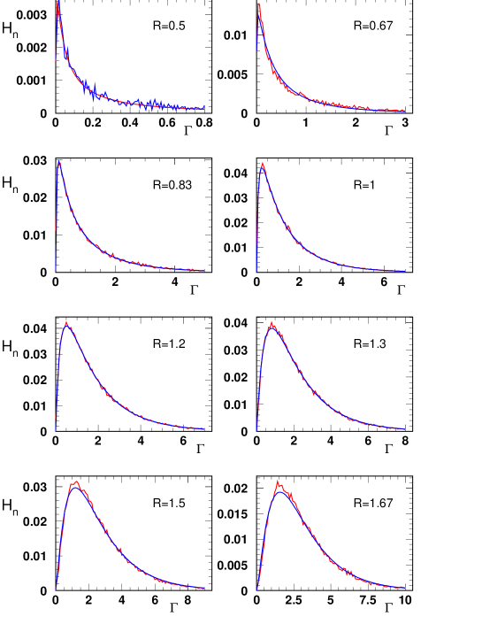
Figure 9: The distributions $H_{n}(\Gamma,\Delta y)$ obtained from JETSET for the default values of the Lund model parameters ($a=0.3$ and $b=0.58$). Also shown are the continuous curves obtained from our fits based on Eq.(38). In this example $\Delta y=6$ and $n=3\dots 10$ . The corresponding $R$ values are shown on each plot.

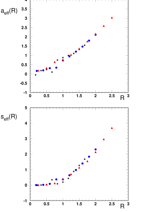
Figure 10: The functions $a_{\mbox{\scriptsize eff}}(R)$ (upper plot) and $s_{\mbox{\scriptsize eff}}(R)$ (lower plot) versus $R$. We show the results for three different rapidity ranges $\Delta y=4$ (triangles), $\Delta y=5$ (circles), and $\Delta y=6$ (stars).

We now examine how the vertices are distributed in $\Gamma$ inside a rapidity range $\Delta y$ for various multiplicities, $n$. Motivated by the finite energy vertex distribution, $H(\Gamma)$, which we considered earlier in Eq.(14), we parameterize the distributions as

$$H_{n}(\Gamma,\Delta y)=C\frac{\Gamma^{a_{\mbox{\scriptsize eff}}(n,\Delta y)}}{(\Gamma+s_{\mbox{\scriptsize eff}}(n,\Delta y))^{a+1}}\exp(-b\Gamma)$$ (38)

Note that taking the weighted average of $H_{n}$ should reproduce the inclusive distribution of Eq.(37). In Fig.(9) we show distributions in $\Gamma$ obtained from JETSET for $\Delta y=6$. Each plot in the figure is for a different number of vertices, $n$, together with the corresponding fit according to Eq.(38). Here the parameters $a_{\mbox{\scriptsize eff}}$ and $s_{\mbox{\scriptsize eff}}$ have been fitted for each different $n$ value. We see that one can find values of $a_{\mbox{\scriptsize eff}}(n,\Delta y)$ and $s_{\mbox{\scriptsize eff}}(n,\Delta y)$ for which a very reasonable description of the $\Gamma$ distributions is obtained. We note that the large $\Gamma$ behaviour is determined only by the Lund parameter $b$ and not by $n$ or $\Delta y$. Thus it is only dependent on the scale for the area law suppression. Next we examine the dependence of both $a_{\mbox{\scriptsize eff}}$ and $s_{\mbox{\scriptsize eff}}$ on the multiplicity and the rapidity interval. We have carried out fits to the $\Gamma$ distribution obtained from JETSET for a set of values of $n$ and $\Delta y$. We find that both of these functions depend only on the ratio $R=n/\Delta y$. This can be seen clearly in Fig.(10) where we plot the results of our fits for three different values of $\Delta y$, as a function of the density $R$.

This completes our study of the distribution of vertices produced in the Lund model of fragmentation. We can summarize our findings as follows. In rapidity the vertices are approximately distributed according to the partition function, whilst in proper time they are distributed according to Eq.(38). Importantly we find that the large $\Gamma$ behaviour of the distribution in $\Gamma$ is determined only by the area law. We also find that the functions $a_{\mbox{\scriptsize eff}}$ and $s_{\mbox{\scriptsize eff}}$ only depend on the density of vertices, $R$, which is itself the important quantity in the equation of state for the gas in rapidity.

5 The particle distributions

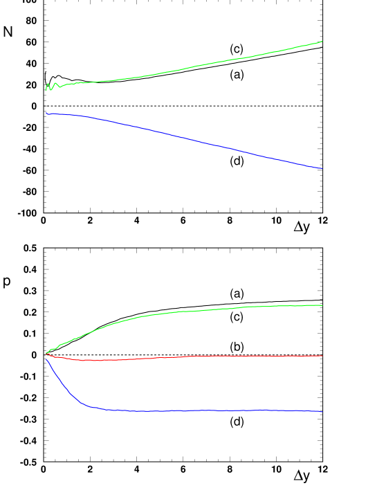
Figure 11: The values of $N$ (upper plot) and $p$ (lower plot) for the particle multiplicity distributions produced by JETSET. The four cases shown correspond to: (a) a single mass, no decays or $p_{\perp}$; (b) complete mass spectra, but no decays or $p_{\perp}$; (c) complete mass spectra, but no decays; and (d) complete mass spectra, charged final state particles.

For primary particles the mean multiplicity corresponds to the mean number of vertices. The effects of going over from vertices to particles essentially means some smearing in rapidity. Thus the rapidity ordering assumed for Eq.(21) will no longer be true. However, for large $\Delta y$ it should still be a good approximation. The rapidity of a particle is distributed around the average rapidity of the two vertices from which the particle stems with a width of about one unit of rapidity. Therefore the particle multiplicity distribution for a finite rapidity interval $\Delta y$ will have the same average as the vertices but a larger width. To understand this effect we return to our simple binomial model. As before we divide the rapidity range into $N$ equal bins with the probability $p$ to contain a vertex. Now we further assume that the presence of a vertex in any bin results in a particle in one of the two neighbouring bins with probability $q$ or in the original bin with the remaining probability $1-2q$. In order to see how this smearing affects the mean and the variance we compute the generating function. The generating function for the original binomial distribution is given by

$$G(z)=[1+p(z-1)]^{N}\;.$$ (39)

Some straightforward algebra then shows that the generating function for the above particle distribution is given by

$$G(z)=[1+p(z-1)]^{(N-2)}[1+p(z-1)+p^{2}(z-1)^{2}q(1-q)]^{2}\;.$$ (40)

Thus two factors of $(1+p(z-1))$ have been modified. The mean is unchanged and equal to $Np$, but the variance is increased from $V=\langle n\rangle(1-p)$ to

$$V=\langle n\rangle[1-p+4pq(1-q)/N]\;.$$ (41)

This distribution can be rather well approximated by another binomial distribution with the same mean and variance. This corresponds to effective $p$ and $N$ values

$$p_{\mbox{\scriptsize eff}} = p[1-4q(1-q)/N]$$

$$N_{\mbox{\scriptsize eff}} = \frac{Np}{p_{\mbox{\scriptsize eff}}}\;.$$ (42)

Thus we see how a larger spread of the particles around the vertices (a larger $q$-value) corresponds to a larger width and a smaller effective $p$-value. From Eq.(42) $p_{\mbox{\scriptsize eff}}$ must be larger than zero, but if we had allowed for a spread beyond the nearest bin then negative values of $p_{\mbox{\scriptsize eff}}$ would be possible. This corresponds to a negative binomial distribution. Since the bin width is of the order of $bm_{\perp}^{2}$ the spread is certainly beyond neighbouring bins in the case of pion production.

We have investigated various cases of final state production. The multiplicity distributions can still be well approximated by binomial distributions with constant $p$-values for large rapidity intervals. In Fig.(11) we show $N$ and $p$ as a function of $\Delta y$ for the various cases.

For a situation with only a single stable hadron, assumed to have the mass $m=0.8$ GeV, and no transverse momentum generation, the result is as expected. Comparing the multiplicity distribution with the distribution for the vertices, we find that $p$ is decreased and $N$ is increased. The product of $N$ and $p$ is however the same for the two distributions.

If we include the standard mixture of different hadron masses $p$ is further reduced. We obtain in this case a distribution that is very close to a Poissonian. Thus, as expected, the width of the multiplicity distribution greatly increases when light pions are produced.

Including transverse momentum generation increases $p$ to positive values as shown in the figure. The transverse mass of the pions is thus, in the case of the standard mixture of hadrons, not small enough to give a negative $p$-value.

Finally, if we include the decays of unstable particles and analyse the final charged particles then the width increases substantially and $p$ becomes negative (corresponding to a negative binomial distribution). Including the final uncharged particles in the analysis results in an even more negative $p$-value.

We can summarize our findings as follows. The width of the multiplicity distribution is very sensitive to the mass spectrum of the produced particles. Using default JETSET the average transverse mass is large enough to give a binomial multiplicity distribution. In this case the negative binomial distribution for the final state stems from the increased width due to decays.

6 Conclusions

Inspired by the Feynman–Wilson gas analogy we have derived an explicit form for the grand partition function of the Lund fragmentation model. This partition function is described in terms of the multiplicity $n$. In particular, we derive an equation of state for the gas, corresponding to the first two terms in the virial expansion in the particle density.

The partition function is derived in the approximation that the particles are ordered in rapidity. This is true for the string break-up vertices and the number of vertices corresponds to the number of particles. Therefore, we have investigated the properties of the partition function using the vertices. For large rapidity intervals, we find that the average and the fluctuations of the multiplicity of vertices are described by the partition function.

The partition function gives a multiplicity distribution which is close to a binomial distribution. We find that the average transverse mass of the produced particles is sufficiently large to get a reasonable description from the approximation that the particles are ordered in rapidity. Thus the multiplicity distribution of the particles stemming from the string is described by an ordinary binomial. It is the decays of the unstable particles that results in a negative binomial distribution for the number of final charged particles.

The distribution of the vertices for different rapidity volumes and different multiplicities has also been investigated in terms of the proper-time. We find that the behaviour for large proper-times is determined only by the area-law and is independent of both the volume and the multiplicity. For smaller proper-times the distribution is described by a simple parametrisation. We find that the important quantity for the parametrisation is the density of vertices in rapidity, which in turn is described by the equation of state for the gas.

Acknowledgment
This work was supported in part by the EU Fourth Framework Programme ‘Training and Mobility of Researchers’, Network ‘Quantum Chromodynamics and the Deep Structure of Elementary Particles’, contract FMRX-CT98-0194 (DG 12 - MIHT).

Appendix A The binomial and negative binomial distributions

The binomial distribution is defined by

$$P(n)=\left(\begin{array}[]{c}N\\ n\end{array}\right)\;p^{n}(1-p)^{N-n}\;.$$ (43)

The average, $\langle n\rangle$, and the variance $V=\langle n^{2}\rangle-\langle n\rangle^{2}$ of this distribution are related to $N$ and $p$ via

$$\langle n\rangle = Np$$

$$V = Np(1-p)\;.$$ (44)

The binomial distributions form a family of distributions depending on the values of $N$ and $p$. In the limit $p\rightarrow 0$ for constant $\langle n\rangle$, the distribution becomes a Poisson distribution. It is also possible to continue the expressions in Eq.(43) to negative $p$-values, which for constant $\langle n\rangle=Np$ implies also a negative $N$. In this case the distribution becomes a negative binomial distribution. Such a distribution is conventionally written in the form

$$P_{k}(n)=\left(\begin{array}[]{c}k+n-1\\ k-1\end{array}\right)\;\tilde{p}^{k}(1-\tilde{p})^{n}$$ (45)

where

$$\tilde{p} = \left(\frac{1}{1-p}\right)\;\;\;\;\;(p<0)$$

$$k = -N\;\;\;\;\;\;\;\;~{}~{}~{}~{}(N<0)\;.$$ (46)

Note that the relationships of Eq. (44) for the average and the variance remain true, even when $p$ and $N$ are both negative. Negative $p$-values correspond to distributions which are wider than a Poissonian. Thus the negative binomial distributions belong to the same larger family as the (ordinary) binomial and Poisson distributions. Within this family the width can vary from zero to infinity. Ordinary and negative binomials correspond to $V$ smaller and larger than $\langle n\rangle$ respectively, with the Poisson distribution as the limiting case in between.

Appendix B The binomial approximation of the partition function

Our aim is to determine the $c_{1}$ and $c_{2}$ parameters of Eq.(35) from the $N$ and $p$ parameters of a binomial distribution. We begin by using Stirlings approximation to write the binomial distribution as

$$\ln(P) = \frac{\ln\!N}{2}+N\ln\!N-(N-n)\ln(N-n)-n-$$ (47)

$$\frac{\ln(N-n)}{2}+N\ln(1-p)+n\ln\left(\frac{p}{1-p}\right)-\ln(n!)$$

whilst the distribution in Eq.(35) can be written as

$$\ln(P_{n})=\ln(c_{0})-\frac{bm^{2}c_{2}n^{2}}{\Delta y}+n\ln(c_{1}\Delta y)-\ln(n!).$$ (48)

We now express $n$ as $n=\langle n\rangle+x$, where $\langle n\rangle$ is the mean. Next we subtract Eq.(47) from Eq.(48) and expand around $x=0$ up to terms of order $x^{2}$. Equating the series coefficients to zero determines the parameters $c_{1}$ and $c_{2}$ in terms of $N$ and $p$. We obtain

$$c_{1}\Delta y = Np\;\exp\left[\frac{1-2p+2Np-2Np^{2}}{2N(1-p)^{2}}\right]$$

$$\frac{bm^{2}c_{2}}{\Delta y} = \frac{2N(1-p)-1}{4N^{2}(1-p)^{2}}$$ (49)

Which for large $\Delta y$ can be simplified to

$$c_{1}\Delta y = Np\;\exp\left[\frac{p}{(1-p)}\right]$$

$$\frac{bm^{2}c_{2}}{\Delta y} = \frac{1}{2N(1-p)}$$ (50)

If we insert these expressions into Eq.(35) then we finally obtain

$$P_{n}\sim\frac{(Np)^{n}}{n!}\exp\left[\frac{-n^{2}+n2Np}{2N(1-p)}\right]$$ (51)