Resummation of soft modes in the free energy of $\Phi^{4}$ theory

Abstract

A new method is proposed for the calculation of the free energy of an $N$-component $\Phi^{4}$ theory at finite temperature. The method combines a perturbative treatment of the hard modes with a non-perturbative treatment in the effectively three-dimensional sector of the soft modes. The separation between hard and soft modes is achieved by the effective field theory method of Braaten and Nieto [1]. One- and two-loop gap equations for the screening mass are used to resum higher order effects in the soft sector. The proposed method is similar to the screened perturbation theory of Karsch, Patkós, and Petreczky [2] albeit avoiding the difficulty of solving gap equations in the full four-dimensional theory. Since gap equations are only used in the three-dimensional effective theory the tedious evaluation of Matsubara sums is not necessary. This simplification makes it possible to go beyond the one-loop gap equation. The large $N$ as well as the finite $N$ case are discussed.

In the last few years there has been a lot of progress in the calculation of the free energy of high temperature field theories [1, 2, 3, 4, 5, 6, 7, 8, 9, 10, 11, 12, 13, 14, 15, 16, 17, 18, 19, 20, 21, 22, 23]. On the perturbative level all corrections to the ideal gas up to order $g^{5}$ have been calculated for gauge theories [3, 4, 5, 6, 7, 8, 9] as well as for scalar $\Phi^{4}$ theory [11, 12, 1]. Unfortunately, these calculations revealed that already for moderate values of the coupling constant higher order corrections become large and oscillating, i.e. each additional higher order correction flips the sign of the deviation from the ideal gas limit (cf. fig. 1). In addition, the results depend crucially on the chosen renormalization point [8, 9].

In this talk I would like to contribute to the question whether/how the perturbative calculation of the free energy can be improved such that one gets a reliable answer not only for very small values of the coupling constant (where perturbation theory works, but there one might use the free (unperturbed) result as well), but also for moderate values of $g$. The aim is to reorganize the loop expansion such that higher loop corrections do not drastically change the result. Of course, it is not clear whether such a reorganization is possible or if one has to rely solely on genuine non-perturbative approaches like lattice calculations [24]. Even for theories where lattice calculations yield reliable results an improved perturbative calculation scheme is nonetheless useful to identify the relevant degrees of freedom of the system. Indeed, the analysis of QCD lattice calculations indicates that at high temperatures the system of massless coupled modes can be very well approximated by a gas of noninteracting massive particles [25, 26, 27, 28]. It is clearly desirable to support this heuristic finding by a calculation starting from first principles such that also the fit parameters (e.g. the temperature dependence of the mass) can be calculated from the underlying theory. In this spirit a reorganization of the loop expansion called screened perturbation theory was suggested in [2] for an $N$-component scalar $\Phi^{4}$ theory.

FIG. 1.: The perturbative result for the free energy density of a one-component massless $g^{2}\Phi^{4}$ theory as a function of the coupling $g$. The label $n$ marks the highest perturbative contribution $\sim g^{n}$ which is taken into account. The free energy density is normalized to its ideal gas value.

Starting from the Lagrangian

$${\cal L}={1\over 2}(\partial\Phi_{i})^{2}+{g^{2}\over 24N}(\Phi_{i}^{2})^{2}$$ (1)

(where $i$ labels the $N$ components of the fields) reorganization of perturbation theory is achieved by adding and subtracting a mass term:

$${\cal L} = {\cal L}_{0}+{\cal L}_{\rm int}\,,$$ (2)

$${\cal L}_{0} = {1\over 2}(\partial\Phi_{i})^{2}+{1\over 2}M^{2}\Phi_{i}^{2}\,,$$ (3)

$${\cal L}_{\rm int} = -{1\over 2}M^{2}\Phi_{i}^{2}+{g^{2}\over 24N}(\Phi_{i}^{2})^{2}\,.$$ (4)

The mass $M$ is calculated from the one-loop gap equation

$$M^{2}=\begin{minipage}[b]{30.00005pt} \begin{figure}\centerline{\hbox{\epsfbox{tadpole.eps}}} \end{figure} \end{minipage}\;.$$ (5)

In [2] the necessary loop calculations were performed up to three loops for the large $N$ case and up to two loops for arbitrary $N$. The result for the free energy density for the large $N$ case is shown in fig. 2 taken from [2]. Obviously the convergence of the screened perturbation theory looks very promising even for large values of the coupling constant.

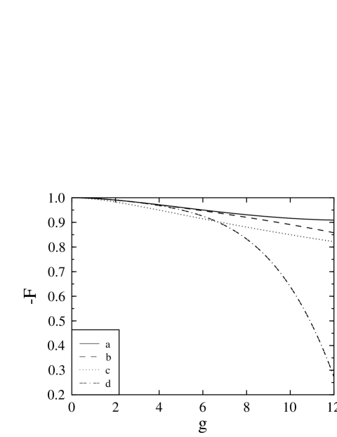
FIG. 2.: The free energy density of the scalar field theory in the large $N$ limit as a function of the coupling constant in units of the free energy density of a massless ideal gas. The curves represent three-loop (a), two-loop (b) and one-loop (c) results of the screened loop expansion as well as the $O(g^{4})$ result (d) of the conventional perturbative expansion. For details see [2] where the figure is taken from.

Of course, it is interesting to check whether this scheme works equally well for arbitrary $N$. There is a technical reason why the three-loop calculations were not performed in [2] for small $N$: It is very complicated to calculate the sunset and the basketball diagram shown in fig. 3 a and b, respectively. While the latter contributes to the free energy, the former shows up as a two-loop correction to the gap equation (5). In the large $N$ limit both diagrams are suppressed by a factor $1/N$. For finite $N$, however, these diagrams have to be taken into account. Unfortunately, to calculate these diagrams with massive propagators is quite messy especially to perform the Matsubara sums.

To circumvent this technical problem the following observation from the QCD case might be useful: If the (oscillating) perturbative corrections to the massless ideal gas are separated in their contributions from the hard (order of temperature $T$) and from the soft (order $gT$) sector [9] one observes that the mentioned oscillatory behavior is mainly caused by the soft modes, i.e. for not too large values of the coupling constant the contribution of the hard modes to the free energy is well behaved while the one from the soft modes is not. The latter, however, can be described by an effective three-dimensional (vacuum like) theory. Hence, if non-perturbative improvements are restricted to the soft mode sector, Matsubara sums do not show up and one can use the techniques of vacuum perturbation theory to calculate the necessary integrals which enter the respective gap equation and the free energy calculation. This consideration is the basis of the work presented here.

FIG. 3.: Sunset (a) and basketball (b) diagram contributing to the gap equation for the mass and to the free energy density, respectively.

The recipe to calculate the free energy density is the following:
1. Disentangle the contributions from different scales (hard and soft).
2. Use conventional perturbation theory to calculate the contribution from the hard scale.
3. Use screened perturbation theory to calculate the contribution from the soft scale.

Fortunately, the first two points have already been performed for one-component $\Phi^{4}$ theory in [1] and for gauge theories in [29]. For simplicity and to compare my results with the four-dimensional screened perturbation theory developed in [2] I will work in the following with an $N$-component $\Phi^{4}$ theory which is a straightforward generalization of the system studied in [1]. The free energy density receives contributions from the hard modes, $F_{h}$, as well as from the soft modes, $F_{s}$. In conventional perturbation theory up to $O(g^{5})$ these contributions are schematically given by

$$F_{h} = \#+\#g^{2}\phantom{+\#g^{3}}+\#g^{4}\phantom{+\#g^{5}}$$ (6)

$$F_{s} = \phantom{\#+\#g^{2}+}\#g^{3}+\#g^{4}+\#g^{5}$$ (7)

The perturbative contribution from the hard sector is given by (cf. [1])

$$F_{h}=F_{h}^{1l}+F_{h}^{2l}+F_{h}^{3l}$$ (8)

with

$$F_{h}^{1l}=-{N\pi^{2}T^{4}\over 90}\,,$$ (9)

$$F_{h}^{2l}={1\over 8}g^{2}(\mu)\tilde{N}{T^{4}\over 12^{2}}\,,$$ (10)

$$F_{h}^{3l}=-{1\over 72}\pi^{2}T^{4}{\tilde{N}\over N}\left({g^{2}\over 16\pi^{2}}\right)^{2}$$ (11)

$$\times \left[{N+8\over 3}\log{\mu\over 4\pi T}+\tilde{N}\gamma+{31\over 15}+4{\xi^{\prime}(-1)\over\xi(-1)}-2{\xi^{\prime}(-3)\over\xi(-3)}\right]\,,$$ (12)

where $\mu$ denotes the renormalization scale, $\tilde{N}$= ($N$+2)/3, $\gamma$ is Euler’s constant, and $\zeta(z)$ is the Riemann zeta function.

The three terms contributing to $F_{s}$ in (7) come from one-, two-, and three-loop diagrams calculated in the effective three-dimensional theory [1]

$${\cal L} = {\cal L}_{0}+{\cal L}_{\rm int}\,,$$ (13)

$${\cal L}_{0} = {1\over 2}(\partial\phi_{i})^{2}+{1\over 2}m^{2}\phi_{i}^{2}\,,$$ (14)

$${\cal L}_{\rm int} = {\lambda\over 24N}(\phi_{i}^{2})^{2}\,.$$ (15)

The so-called short distance coefficients $m$ and $\lambda$ in this theory for the soft modes are influenced by the interaction with the hard modes. Perturbatively they are given by

$$\lambda=g^{2}T+o(g^{4})$$ (16)

and

$$m^{2}={1\over 24}{\tilde{N}\over N}g^{2}(\mu)T^{2}\left\{1+{g^{2}\over 16\pi^{2}}\left[-{N+8\over 3N}{\rm ln}{\mu\over 4\pi T}\right.\right.$$ (18)

$$\left.\left.+{4\over N}{\rm ln}{\Lambda\over 4\pi T}-{\tilde{N}\over N}\gamma+{2\over N}+{2\over N}{\xi^{\prime}(-1)\over\xi(-1)}\right]+o(g^{4})\right\}$$

where the higher order corrections do not influence the result for the free energy up to $O(g^{5})$. Here a new parameter shows up, the separation scale $\Lambda$ which separates the hard from the soft modes. $\Lambda$ serves also as the renormalization scale in the three-dimensional theory, i.e. it appears in the course of renormalizing logarithmic ultraviolet divergences from loop integrals. Note that the short distance coefficient $m$ is not a physical quantity. If physical quantities (like the free energy or the screening mass) are calculated in conventional perturbation theory the dependence of the short distance coefficients on $\Lambda$ exactly cancels in every order of $g$ the $\Lambda$ dependence coming from the renormalization of loops [1]. Going beyond a perturbative calculation in the following a dependence on $\Lambda$ will remain. This will be discussed below.

According to point 2 of my recipe I will keep the perturbative results caused by the hard modes, i.e. the results for $F_{h}$, $m$ and $\lambda$, while according to point 3 I will replace the three terms of $F_{s}$ given in (7) by the one-, two-, and three-loop result of (three-dimensional) screened perturbation theory

$${\cal L} = {\cal L}_{0}+{\cal L}_{\rm int}\,,$$ (19)

$${\cal L}_{0} = {1\over 2}(\partial\phi_{i})^{2}+{1\over 2}M^{2}\phi_{i}^{2}\,,$$ (20)

$${\cal L}_{\rm int} = -{1\over 2}(M^{2}-m^{2})\phi_{i}^{2}+{\lambda\over 24N}(\phi_{i}^{2})^{2}\,.$$ (21)

The Feynman diagrams which have to be calculated are depicted in fig. 4. The cross denotes the counter term

$$\delta m^{2}=M^{2}-m^{2}$$ (22)

(times $-1$). There is an additional counter diagram not shown in fig. 4 which serves to renormalize the mass. It cancels the singularity arising from the basketball diagram. It also yields a finite contribution to the three-loop result given below. For details of the calculation cf. [30]. The result for the contribution of the (resummed) soft modes to the free energy density is

$$F_{s}=T\,(f_{s}^{1l}+f_{s}^{2l}+f_{s}^{3l})$$ (23)

with

$$f_{s}^{1l}=-{1\over 12\pi}NM^{3}\,,$$ (24)

$$f_{s}^{2l}={1\over 8\pi}\tilde{N}{\lambda\over 16\pi}M^{2}+{1\over 8\pi}N\delta m^{2}M\,,$$ (25)

$$f_{s}^{3l}=-{1\over 8\pi}{\tilde{N}^{2}\over N}\left({\lambda\over 16\pi}\right)^{2}M-{1\over 8\pi}\tilde{N}{\lambda\over 16\pi}\delta m^{2}$$ (27)

$$-{1\over 32\pi}N(\delta m^{2})^{2}{1\over M}+{1\over 3\pi}{\tilde{N}\over N}\left({\lambda\over 16\pi}\right)^{2}M\left({\rm ln}{\Lambda\over 4M}+{3\over 2}\right)\,.$$

where the appearance of a cross in a diagram is treated as being a loop, i.e. the third diagram of fig. 4 is a two-loop contribution and the fifth and sixth diagram are three-loop contributions.

FIG. 4.: Feynman diagrams for the free energy contributions to be calculated in three-dimensional screened perturbation theory with massive propagators with mass $M$. The cross denotes a counter term $-\delta m^{2}$.

The final result for the free energy density is

$$F=F_{h}+F_{s}$$ (28)

where $F_{h}$ is given by (8-11) and $F_{s}$ by (23-27) with the parameters given in (16,18,22). By inspecting these equations we find that $F$ depends on the temperature $T$, the coupling constant $g$, the renormalization scale (of the full four-dimensional theory) $\mu$, the separation scale $\Lambda$, and on the so far unspecified mass $M$. In a full calculation of the free energy density only the dependence on $T$ and $g$ would remain. In an approximate calculation, however, there is an additional dependence on the other three parameters and appropriate values have to be chosen for them. Since I am mainly interested in the soft mode sector and in a proper choice for $M$ I will determine $\mu$ and $\Lambda$ in a very simple way: I require that perturbation theory in the hard mode sector works optimal, i.e. I will choose $\mu$ and $\Lambda$ such that the $g^{4}$ contributions to $F_{h}$, given in (11), and $m$, given in (18), vanish. This fixes the separation scale to

$$\Lambda=4\pi T{\rm exp}\left(-{61\over 60}-{3\over 2}{\zeta^{\prime}(-1)\over\zeta(-1)}+{1\over 2}{\zeta^{\prime}(-3)\over\zeta(-3)}\right)\approx 0.32T$$ (29)

while the renormalization scale becomes

$$\mu = 4\pi T{\rm exp}\left[{1\over N+8}\left(-(N+2)\gamma-{31\over 5}\right.\right.$$ (31)

$$\left.\left.\phantom{4\pi T{\rm exp}m{1\over N+8}}-12{\zeta^{\prime}(-1)\over\zeta(-1)}+6{\zeta^{\prime}(-3)\over\zeta(-3)}\right)\right]\,.$$

This yields e.g.

$$\mu\approx 1.12\cdot 2\pi T\quad\mbox{for}\,\,N\to\infty$$ (32)

and

$$\mu\approx 0.57\,T\quad\mbox{for}\,\,N=1\,.$$ (33)

Admittedly, the chosen value for $\mu$ is somewhat low for the case $N=1$ since it is usually supposed to be somewhere around $2\pi T$ (cf. [1, 9, 18]). However, changing $\mu$ or $\Lambda$ does not qualitatively change the results to be presented in the following.

Of course, the crucial question now is how to determine $M$ such that large perturbative contributions from higher loops are resummed in the tree level mass $M$. I will explore two different resummation procedures:
The first one is based on the principle of minimal sensitivity (see e.g. [31] and references therein). Since the full calculation for the free energy is independent of $M$ it might be reasonable to look for an extremum of the approximate result with respect to $M$, i.e.

$${\partial F\over\partial M}=0\qquad\mbox{(POMS)}\,.$$ (34)

The second resummation procedure is based on the criterion of fastest apparent convergence (see e.g. [31] and references therein). Here, an appropriate quantity is chosen, calculated in two different orders of the approximation scheme, and it is required that the difference vanishes. I will use the inverse propagator evaluated at momentum $\vec{k}^{2}=-M^{2}$ and take the difference of the results for the zeroth and the first/second order. Since the free inverse propagator vanishes at this momentum this simply means that the self energy is demanded to vanish at $\vec{k}^{2}=-M^{2}$. Taking the second order result for the self energy, i.e. up to two loops, corresponds to the evaluation of the free energy up to three loops. This yields the gap equation (see also [31, 32, 33, 34, 35, 36] and references therein)

$$M^{2}-m^{2}=\raisebox{-7.5pt}{\begin{minipage}[b]{150.00023pt} \begin{figure}\centerline{\hbox{\epsfbox{feyntlg.eps}}} \end{figure} \end{minipage}}|_{\vec{k}^{2}=-M^{2}}\,.$$ (35)

If the calculation of the free energy is restricted to maximal two loops the corresponding one-loop gap equation results from (35) by simply dropping the last three diagrams. Again, there is an additional counter term not shown in (35) which renormalizes the mass. It cancels the singularity arising from the sunset diagram. For details of the calculation see [30]. The result for the two-loop gap equation (TLG) is

$$0 = \delta m^{2}+2{\lambda\over 16\pi}{\tilde{N}\over N}M-{\lambda\over 16\pi}{\tilde{N}\over N}{\delta m^{2}\over M}-2\left({\lambda\over 16\pi}\right)^{2}{\tilde{N}^{2}\over N^{2}}$$ (37)

$$+{8\over 3}\left({\lambda\over 16\pi}\right)^{2}{\tilde{N}\over N^{2}}\left({\rm ln}{\Lambda\over 8M}+{3\over 2}\right)\qquad\mbox{(TLG)}\,.$$

For the one-loop gap equation (OLG) all terms on the right hand side except the first two have to be dropped.

Both schemes to determine $M$ resulting in (34) and (37), respectively, might yield more than one solution for $M$. I always take the one which is continuously connected to the perturbative result ($M^{2}\approx m^{2}$). If the calculation of the free energy is restricted to maximal two loops the principle of minimal sensitivity yields the same result as the one-loop gap equation. In the large $N$ limit the sunset diagram (the last one in (35)) is suppressed. There TLG, OLG, and POMS yield identical results. This is easy to understand, if one recalls that for $N\to\infty$ the tadpole resummation (which is already achieved by OLG) is sufficient to solve the exact Dyson-Schwinger equation for the propagator [37]. If the solution for $M$ is inserted in (23-27) the three-loop contribution $f_{s}^{3l}$ exactly vanishes in the large $N$ limit. The same is true for all higher loop contributions not calculated here (see also [17, 19]).

For the presentation of the results one has to make a decision how to sort the various contributions $F_{h}^{1l}$, $F_{h}^{2l}$, $F_{h}^{3l}$, $f_{s}^{1l}$, $f_{s}^{2l}$, and $f_{s}^{3l}$. One might be tempted to sort them in numbers of loops such that the lowest order approximation to the free energy density would be $F_{h}^{1l}+Tf_{s}^{1l}$, the next one $F_{h}^{1l}+Tf_{s}^{1l}+F_{h}^{2l}+Tf_{s}^{2l}$, and so on. This, however, I think is misleading in view of the schematic picture of the perturbative contributions given in (6,7) and the fact that the contributions $f_{s}^{1l}$, $f_{s}^{2l}$, and $f_{s}^{3l}$ only improve the soft perturbative $g^{3}$, $g^{4}$, and $g^{5}$ contributions, respectively. Therefore, I choose the following sequence of approximations:

$$F_{0} = F_{h}^{1l}\,,$$ (38)

$$F_{2} = F_{h}^{1l}+F_{h}^{2l}\,,$$ (39)

$$F_{3} = F_{h}^{1l}+F_{h}^{2l}+Tf_{s}^{1l}\,,$$ (40)

$$F_{4} = F_{h}^{1l}+F_{h}^{2l}+Tf_{s}^{1l}+F_{h}^{3l}+Tf_{s}^{2l}\,,$$ (41)

$$F_{5} = F_{h}^{1l}+F_{h}^{2l}+Tf_{s}^{1l}+F_{h}^{3l}+Tf_{s}^{2l}+Tf_{s}^{3l}\,.$$ (42)

Note that for the results shown below the renormalization scale $\mu$ is chosen such that $F_{h}^{3l}$ vanishes. Therefore the difference between $F_{3}$ and $F_{4}$ is solely due to $f_{s}^{2l}$.

A second question which has to be clarified is which $M$ is taken for which order of the approximation. Concerning the principle of minimal sensitivity for the approximation $F_{5}$, clearly, the mass $M$ has to be determined from (34) with the input $F=F_{5}$. With the resulting mass, $F_{5}$ can be evaluated as a function of the coupling constant $g$ (and the temperature $T$). One might take the same mass for the evaluation of $F_{4}$. However, I think it is more appropriate here to use only $F=F_{4}$ as an input in (34). This philosophy, however, does not work for $F_{3}$. Since $f_{s}^{1l}$ is proportional to $M^{3}$, POMS would yield $M=0$, i.e. no difference between the approximations $F_{2}$ and $F_{3}$. This is, of course, not very useful. Therefore I break the rule for this special case and use for the evaluation of $F_{3}$ the value for $M$ resulting from (34) with $F=F_{4}$ as input.

FIG. 5.: Various approximations $F_{n}$ (labeled with $n$) to the free energy density of an $N$-component $\Phi^{4}$ theory as a function of the coupling $g$ in the large $N$ limit. See main text for details. The free energy density is normalized to its ideal gas value $F_{0}$. The dashed lines show the perturbative approximations $O(g^{3})$, $O(g^{5})$, $O(g^{4})$ (top to bottom).

For the criterion of fastest apparent convergence and its resulting one- and two-loop gap equations I will use the result of TLG for the evaluation of $F_{5}$ and of OLG for the evaluation of $F_{4}$. Again, it is not clear which $M$ should be used for $F_{3}$. I will use the result of OLG here.

The results for $F_{0}$ - $F_{5}$ are shown in fig. 5 for the case $N\to\infty$ and in figs. 6 and 7 for $N=1$. To make the two cases comparable the respective maximal value of $g$ is chosen such that the short distance coefficient $m$ given in (18) is approximately the same for both cases. For the large $N$ case I can reproduce the results of [2] (cf. fig. 2): Perturbation theory is improved by the resummation scheme; even for large values of the coupling constant the best approximation (full line in fig. 2, $F_{5}$ in fig. 5) is quite near to the ideal gas limit (about 10% deviation for $g=12$); the screening mass $M$ (not shown) equals the perturbative one-loop result for small coupling constants ($g^{2}$ part of the short distance coefficient (18)) and is about half of it for $g=12$.

FIG. 6.: Various approximations $F_{n}$ (labeled with $n$) to the free energy density of a one-component $\Phi^{4}$ theory as a function of the coupling $g$ using the criterion of fastest apparent convergence. See main text for details. The free energy density is normalized to its ideal gas value $F_{0}$. “pert” labels the perturbative approximation $O(g^{5})$.

Unfortunately, the picture is quite different for the case $N=1$. Comparing the purely perturbative results (fig. 1) with the ones obtained in the resummation schemes (figs. 6, 7) it turns out that the criterion of fastest apparent convergence (fig. 6) does not improve the loop expansion at all. The principle of minimal sensitivity improves the loop expansion. However, it is striking that also in this scheme for larger values of the coupling constant the approximate value for the free energy density changes from $|F|<|F_{0}|$ to $|F|>|F_{0}|$ when proceeding from the fourth to the fifth approximation. This seems to resemble the oscillatory behavior of the perturbative results. Obviously, there is a window between $g\approx 3$ and $g\approx 5$ where the latter resummation scheme (POMS) shows a promising convergence behavior and improves the perturbative results. (Below $g\approx 3$ one might trust the perturbative results as well.) However, the fact that the two discussed resummation schemes yield quite different results raises doubts on the reliability of both.

FIG. 7.: Same as fig. 6 but using the principle of minimal sensitivity.

Before discussing the possible lessons one could learn from the three-dimensional version of resummed perturbation theory let me recall the additional assumptions which enter the presented method besides the general idea of resumming the soft modes only: First of all, I had to choose the values for the renormalization scale $\mu$ and the separation scale $\Lambda$. I have used a very simple recipe here to fix these quantities by demanding that the $g^{4}$ contributions to the hard mode quantities $F_{h}$ and $m$ have to vanish (cf. (29-33) and discussion there). It is worth noting that this approach is in accordance with the criterion of fastest apparent convergence which I have used later on. In principle, if perturbation theory works these $g^{4}$ contributions would be small but in general would not completely vanish. Therefore, forcing them to vanish by choosing the scales accordingly might cause other contributions to become unnaturally large. On the other hand, this simple choice allows to discuss in the cleanest way the convergence behavior of the soft mode sector and its influence on the total result for the free energy. If e.g. $\mu$ is chosen in another way then the influence of $f_{s}^{2l}$ and $f_{s}^{3l}$ in (41,42) would intertwine with the influence of $F_{h}^{3l}$. Nonetheless, it is important to check whether at least the qualitative results are robust against changes in $\mu$ and $\Lambda$. Therefore, I will now explore other choices for the scale parameters. I will restrict myself to the most interesting case $N=1$.

Concerning the renormalization scale a reasonable choice might be $\mu=2\pi T$ since this is the typical energy scale of the hard modes [1, 9, 18]. For this case the contribution of the hard modes to the free energy (8) becomes (for $N=1$)

$$F_{h}\approx F_{h}^{1l}\left[1-0.0079\,g^{2}\left(1-0.046\,g^{2}\right)\right]\quad\mbox{for}\quad\mu=2\pi T\,.$$ (43)

One finds that the $g^{4}$ contribution overwhelms the $g^{2}$ contribution already for $g\approx 4.7$. In view of the large coupling constants I have dealt with in this work (up to $g=7$ for $N=1$) this choice of $\mu$ is inappropriate since in this case the naive perturbation theory which I have used in the hard mode sector breaks down. For the more naive choice $\mu=T$ one gets a $g^{4}$ coefficient which is somewhat smaller:

$$F_{h}\approx F_{h}^{1l}\left[1-0.0079\,g^{2}\left(1-0.011\,g^{2}\right)\right]\quad\mbox{for}\quad\mu=T\,.$$ (44)

For this choice of $\mu$ (and $\Lambda$ as given in (29)) the free energy contributions are plotted in fig. 8 using the principle of minimal sensitivity which for the original choice of $\mu$ was the better one as compared to the criterion of apparent convergence. Obviously, also for this choice of the renormalization scale POMS improves the convergence as compared to the perturbative loop expansion. However, one finds qualitatively the same feature as in fig. 7, namely the oscillatory behavior around the ideal gas limit for coupling constants larger than $g\approx 5$. Note, however, that the fourth and fifth approximation basically have now exchanged their places as compared to fig. 7.

FIG. 8.: Same as fig. 6 but using the principle of minimal sensitivity and $\mu=T$.

Concerning the separation scale it is reasonable to put it somewhere between the typical energy scales of the hard and the soft modes. While the former is $2\pi T$ as discussed above the latter is characterized by $m$ or roughly the lowest perturbative ($g^{2}$) contribution to $m$ (as long as perturbation theory holds for the hard mode sector):

$$m_{1l}^{2}:={1\over 24}{\tilde{N}\over N}g^{2}(\mu)T^{2}\,.$$ (45)

Thus a reasonable choice is

$$\Lambda=\sqrt{2\pi T\,m_{1l}}\sim\sqrt{g}\,.$$ (46)

Fig. 9 shows the free energy contributions for this choice of the separation scale (and $\mu$ as given in (33)) using again the principle of minimal sensitivity. Comparing the values for $F_{5}$ from fig. 7 and fig. 9 shows that the latter choice for the separation scale (46) makes the convergence behavior worse. In addition, it turns out that in this case the full POMS condition, i.e. using $F=F_{5}$ in (34), does not have a solution for $M$ for coupling constants smaller than $g\approx 2$. Therefore, in fig. 9 $F_{5}$ is plotted only for $g>2$ (hardly visible). All of this is qualitatively in line with the general finding that the presented resummation scheme does not improve the loop expansion for the case $N=1$.

FIG. 9.: Same as fig. 6 but using the principle of minimal sensitivity and $\Lambda=\sqrt{2\pi T\,m_{1l}}$.

Besides the specific choices for the renormalization and separation scales I have tacitly assumed that there is only one counter term (22) in (20). Alternatively one could introduce an additional counter term for each additional loop order. This approach will be discussed in more detail in [30]. Qualitatively this modified method yields the same results as presented here. Especially no further improvement concerning the poor convergence behavior for $N=1$ is achieved by this modification.

To summarize, I have found that a scheme which combines conventional perturbation theory for the hard modes with screened perturbation theory for the soft modes significantly improves conventional perturbation theory for an $N$-component $\Phi^{4}$ theory in the large $N$ limit. Contrary, this scheme does not work equally well for finite $N$. There are several possibilities to explain this shortcoming:

1. The presented scheme is based on the assumption that the hard and the soft modes can be separated and that the screening effect can be neglected for the hard modes. The necessary condition for this assumption to hold is that in the Matsubara propagator $1/(\vec{k}^{2}+(2n\pi T)^{2}+M^{2})$ the mass term can be neglected compared to the temperature term for $n\neq 0$, i.e.

$$M^{2}\ll(2\pi T)^{2}\,.$$ (47)

If the screening mass does not fulfill this condition the presented scheme would not be appropriate. In turn, if screened perturbation theory works in the four-dimensional theory and yields a screening mass which fulfills (47) then also my three-dimensional version of screened perturbation theory should work. Of course, I cannot say what the true value for the screening mass is. However, I can at least check whether the result for $M$ obtained in my approximation scheme is consistent with the underlying assumption (47). Fig. 10 shows the results for $M$ for the different resummation schemes. The line labeled with “POMS” is obtained from (34) using the “best” result $F=F_{5}$ from (42). The “TLG” and “OLG” lines result from (37) with the appropriate terms dropped in the latter case. I think it is fair to say that the POMS and OLG results fulfill (47) in the plotted regime for the coupling constant. For the TLG result relation (47) is not very well satisfied for the largest plotted values of the coupling constant. However, for $g\approx 5$ there is a factor of about 40 between $M^{2}$ and $(2\pi T)^{2}$ so that (47) is roughly fulfilled. Fig. 6 shows that already here the convergence of the resummation scheme is worse than the conventional perturbative scheme. Thus, the failure of the resummation scheme utilizing the criterion of fastest apparent convergence cannot be traced back to its inconsistency with the underlying assumption (47).

2. Another reason for the finding that the presented resummation scheme does not work equally well for $N\to\infty$ and $N=1$ may be that only a momentum independent mass is resummed. It might appear that the resummation of a more general, i.e. momentum dependent self energy (as e.g. advocated in [17]) would be more appropriate. For the large $N$ case this would not change anything since the sunrise diagram and all higher momentum dependent diagrams are suppressed by powers of $1/N$. As already pointed out before, the resummation of tadpoles is the only thing which has to be done in the large $N$ limit. If the possible momentum dependence is a necessary ingredient for a reliable resummation scheme then this would naturally explain why the scheme presented here works for $N\to\infty$ but fails for $N=1$. I will elaborate on this question in [30].

3. Besides its momentum dependence the sunrise diagram (and the corresponding basketball diagram contributing to the free energy) gives rise to a logarithmic term in the mass $M$. One may argue that this logarithmic term via an inappropriately large contribution ${\rm ln}(\#\Lambda/M)$ shifts the mass to a wrong place and causes a breakdown of the three-dimensional screened perturbation theory. Since this logarithmic term is caused by the renormalization of the theory it might be possible to handle that problem by renormalization group equations (cf. e.g. [1]). Of course, this is a pure speculation so far and deserves further studies. If it is true it would also explain why the resummation works in the large $N$ limit. There, these logarithmic contributions are suppressed as one can easily check by inspecting (27) and (37).

FIG. 10.: The resummed mass $M$ as obtained from POMS, TLG, and OLG and the short distance coefficient $m$ as a function of the coupling $g$ for a one-component $\Phi^{4}$ theory. See main text for details.

4. The most negative explanation for the shortcomings of the presented resummation scheme would be that the concept of screened perturbation theory does not work at all (or only for very special cases like the large $N$ limit) or more generally that concerning the determination of the free energy there is so far no method which reorganizes the loop expansion in a useful way, at least for coupling constants which are not tiny. This would imply that we have to rely on genuine non-perturbative approaches like lattice calculations. Indeed, the free energy density is a quantity which can be calculated on the lattice (see e.g. [38, 39]). However, for many other, e.g. non-static quantities there are fundamental obstacles which so far prevent their evaluation on the lattice. If (improved) perturbation theory fails to calculate the free energy density one may also doubt the results for other quantities obtained in a loop expansion in high temperature quantum field theory.

I conclude that the question how to reliably calculate the free energy density in a modified loop expansion is still open.

REFERENCES

- [1] E. Braaten and A. Nieto, Phys. Rev. D51, 6990 (1995).
- [2] F. Karsch, A. Patkós, and P. Petreczky, Phys. Lett. B401, 69 (1997).
- [3] C. Coriano and R.R. Parwani, Phys. Rev. Lett. 73, 2398 (1994).
- [4] R.R. Parwani, Phys. Lett. B334, 420 (1994), Erratum-ibid. B342, 454 (1995).
- [5] R.R. Parwani and C. Coriano, Nucl. Phys. B434, 56 (1995).
- [6] P. Arnold and C. Zhai, Phys. Rev. D50, 7603 (1994).
- [7] P. Arnold and C. Zhai, Phys. Rev. D51, 1906 (1995).
- [8] C. Zhai and B. Kastening, Phys. Rev. D52, 7232 (1995).
- [9] E. Braaten and A. Nieto, Phys. Rev. D53, 3421 (1996).
- [10] M. Achhammer, U. Heinz, S. Leupold, and U.A. Wiedemann, Ann. Phys. (NY) 261, 1 (1997).
- [11] J. Frenkel, A.V. Saa, and J.C. Taylor, Phys. Rev. D46, 3670 (1992).
- [12] R. Parwani and H. Singh, Phys. Rev. D51, 4518 (1995).
- [13] F. Karsch, M. Lütgemeier, A. Patkós, and J. Rank, Phys. Lett. B390, 275 (1997).
- [14] B. Kastening, Phys. Rev. D56, 8107 (1997).
- [15] T. Hatsuda, Phys. Rev. D56, 8111 (1997).
- [16] I.T. Drummond, R.R. Horgan, P.V. Landshoff, and A. Rebhan, Phys. Lett. B398, 326 (1997).
- [17] J. Reinbach and H. Schulz, Phys. Lett. B404, 291 (1997).
- [18] I.T. Drummond, R.R. Horgan, P.V. Landshoff, and A. Rebhan, Nucl. Phys. B524, 579, (1998).
- [19] A. Peshier, B. Kämpfer, O.P. Pavlenko, and G. Soff, Europhys. Lett. 43, 381 (1998).
- [20] B. Vanderheyden and G. Baym, hep-ph/9803300.
- [21] D. Bödeker, P.V. Landshoff, O. Nachtmann, and A. Rebhan, hep-ph/9806514.
- [22] A. Rebhan, these proceedings, hep-ph/9808480.
- [23] H. Schulz, these proceedings, hep-ph/9808339.
- [24] M. Creutz, Quarks, Gluons, and Lattices (Cambridge University Press, Cambridge, 1983).
- [25] F. Karsch, Nucl. Phys. B9 [Proc. Suppl.] 357 (1989).
- [26] V. Goloviznin and H. Satz, Z. Phys. C57, 671 (1993).
- [27] A. Peshier, B. Kämpfer, O.P. Pavlenko, and G. Soff, Phys. Rev. D54, 2399 (1996).
- [28] P. Levai and U. Heinz, Phys. Rev. C57, 1879 (1998).
- [29] K. Farakos, K. Kajantie, K. Rummukainen, and M. Shaposhnikov, Nucl. Phys. B425, 67 (1994).
- [30] S. Leupold, in preparation.
- [31] S. Chiku and T. Hatsuda, Phys. Rev. D58, 076001, (1998).
- [32] R.O. Ramos, Braz. J. Phys. 26, 684 (1996), hep-ph/9607416.
- [33] A. Patkós, P. Petreczky, and Zs. Szép, Eur. Phys. J. C5, 337 (1998).
- [34] F. Eberlein, Phys. Lett. B439, 130 (1998).
- [35] P. Petreczky, these proceedings, hep-ph/9809414.
- [36] S. Chiku, these proceedings, hep-ph/9809215.
- [37] L. Dolan and R. Jackiw, Phys. Rev. D9, 3320 (1974).
- [38] C. DeTar, in Quark-Gluon Plasma 2, p. 1, edited by R.C. Hwa (World Scientific, Singapore, 1995).
- [39] E. Laermann, Nucl. Phys. A610, 1c (1996).