Abstract

We determine the full structure of the leading (double-pole) divergences of $O(p^{6})$ in the meson sector of chiral perturbation theory. The field theoretic basis for this calculation is described. We then use an extension of this result to determine the $p^{6}$ contributions containing double chiral logarithms ($L^{2}$), single logarithms times $p^{4}$ constants ($L\times L_{i}^{r}$) and products of two $p^{4}$ constants $(L_{i}^{r}\times L_{j}^{r})$ for $F_{\pi}$, $F_{K}/F_{\pi}$, $K_{l3}$ and $K_{e4}$ form factors. Numerical results are presented for these quantities.

* Work supported in part by TMR, EC-Contract No. ERBFMRX-CT980169
(EURODA$\Phi$NE).
^# Address after september 1 1998: Institut für Theoretische Physik der Universität Zürich, Winterthurerstr. 190, CH–8057 Zürich–Irchel.

1.

Chiral logs arise in the process of renormalization. For instance, in dimensional regularization a renormalization scale $\mu$ is introduced to ensure the correct dimension of amplitudes in $d$ dimensions. One-loop divergences then always appear in the scale independent combination

$${\cal X}=\displaystyle\frac{\mu^{d-4}}{(4\pi)^{2}}\left[{1\over d-4}+{1\over 2}\ln{M^{2}\over\mu^{2}}+\dots\right]$$ (1)

with a characteristic meson mass $M$. Renormalization consists in canceling the pole in $d-4$ by the divergent part of the tree-level amplitude of $O(p^{4})$ and replacing it by a combination of scale dependent low-energy constants from ${\cal L}_{4}$, the next-to-leading term in the low-energy expansion of the effective chiral Lagrangian ${\cal L}_{\rm eff}={\cal L}_{2}+{\cal L}_{4}+{\cal L}_{6}+\dots$. In many cases, the chiral logs $\ln{M^{2}/\mu^{2}}$ make sizable contributions for a typical scale $\mu$ of $O(M_{\rho})$.

At $O(p^{6})$, the leading divergences are double poles accompanied by double chiral logs, the leading infrared singularities of $O(p^{6})$. The double logs are again numerically important in general, e.g., for $S$-wave threshold parameters in $\pi\pi$ scattering [1, 2]. As a by-product of the complete renormalization of the generating functional of $O(p^{6})$ [3], we present here the double chiral logs in full generality for chiral $SU(n)$. As will be shown below, the double logs ($L^{2}$) come together with terms of the form $L\times L_{i}^{r}$ and products $L_{i}^{r}\times L_{j}^{r}$ where the $L_{i}^{r}$ are the renormalized low-energy constants of $O(p^{4})$ (we use the $SU(3)$ notation here for simplicity). It is then very natural to include such terms in the numerical analysis especially because they are often comparable to or even bigger than the proper double-log terms.

The purpose of this letter is twofold. First, our general double-pole divergence Lagrangian for $SU(n)$ may serve as a check of existing and yet to be performed two-loop calculations of $O(p^{6})$. Secondly, the numerical analysis may provide hints as to where large $p^{6}$ corrections are to be expected. Of course, the partial $p^{6}$ results presented here are not a substitute for the full expressions of $O(p^{6})$. But once the double-pole divergence Lagrangian has been determined from a one-loop calculation (see below), the numerical applications come at almost no cost compared to the full $p^{6}$ calculations.

2.

In a mass independent regularization scheme like dimensional regularization, the divergent parts are polynomials in masses and external momenta. In the present case, the coefficients of those polynomials are renormalized by the general chiral Lagrangian of $O(p^{6})$. Therefore, the divergences themselves can be cast into the form of ${\cal L}_{6}$ with divergent coefficients that receive contributions from the diagrams shown in Fig. 1.

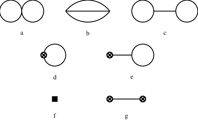
Figure 1: Diagrams contributing to the generating functional of $O(p^{6})$. The propagators and vertices carry the full tree structure associated with the lowest–order Lagrangian ${\cal L}_{2}$. Normal vertices are from ${\cal L}_{2}$, crossed circles denote vertices from ${\cal L}_{4}$ and the square in diagram f stands for a vertex from ${\cal L}_{6}$.

There are two types of diagrams in Fig. 1, reducible and irreducible ones, both divergent in general. However, as will be shown below, one can always choose ${\cal L}_{4}$ in such a way as to make the sum of the reducible diagrams c,e,g finite. Even so, these diagrams give rise to double logs in general. These double logs are completely determined by the tree-level contribution g proportional to products of low-energy constants of $O(p^{4})$.

The tree-level diagram f being trivial, we are left with the irreducible loop diagrams a,b,d in Fig. 1. Starting with the two-loop diagrams a, b, the corresponding divergences in a given coefficient of ${\cal L}_{6}$ are of the general form

$$x(d)\displaystyle\frac{\mu^{2(d-4)}}{(4\pi)^{4}}\left[{1\over d-4}+{1\over 2}\ln{M^{2}\over\mu^{2}}+\dots\right]^{2}$$ (2)

$$= x(d)\displaystyle\frac{\mu^{2(d-4)}}{(4\pi)^{4}}\left[{1\over(d-4)^{2}}+\displaystyle\frac{\ln{M^{2}/\mu^{2}}}{d-4}+{1\over 4}(\ln{M^{2}\over\mu^{2}})^{2}+\dots\right]$$

where $x(d)$ is a function of $d$ that depends on the specific coefficient under consideration.

The problematic piece in (2) is the nonlocal divergence ${x_{0}\ln{M^{2}/\mu^{2}}}/({(4\pi)^{4}(d-4)})$ that cannot be renormalized with a local action of $O(p^{6})$. Here, $x_{0}$ is the leading coefficient in the Taylor expansion of $x(d)$ around $d=4$: $x(d)=x_{0}+x_{1}(d-4)+\cdots~{}.$ Therefore, in accordance with general theorems of renormalization theory [4], the nonlocal divergence must cancel with other contributions. Since the sum of reducible diagrams in Fig. 1 is finite with our choice of ${\cal L}_{4}$, the cancellation can only come from diagram d that is proportional to the low-energy constants $L_{i}$ . These constants are themselves divergent (to renormalize the one-loop divergences). In $d$ dimensions, they can be written

$$L_{i}(d)=\mu^{d-4}\left[\displaystyle\frac{\Gamma_{i}}{(4\pi)^{2}(d-4)}+L_{i}^{r}(\mu)+\dots\right]$$ (3)

with known coefficients $\Gamma_{i}$ and renormalized constants $L_{i}^{r}(\mu)$ [5]. The divergences due to the one-loop diagram d in Fig. 1 are then given by the product of (1) and (3) with appropriate coefficients $y_{i}(d)$:

$$-{y_{i}(d)\over 2}{\cal X}L_{i}(d) = -{y_{i}(d)\over 2}\displaystyle\frac{\mu^{2(d-4)}}{(4\pi)^{4}}\left[{\Gamma_{i}\over(d-4)^{2}}+\displaystyle\frac{\Gamma_{i}\ln{M^{2}/\mu^{2}}}{2(d-4)}+\displaystyle\frac{(4\pi)^{2}L_{i}^{r}(\mu)}{d-4}\right.$$ (4)

$$+ \left.{(4\pi)^{2}\over 2}L_{i}^{r}(\mu)\ln{M^{2}/\mu^{2}}+\dots\right]~{}.$$

Summation over $i$ is implied and we have chosen the numerical factor $-1/2$ in (4) to conform to the notation of Ref. [2]. Cancellation of the nonlocal divergences in (2) and (4) is guaranteed by Weinberg’s conditions [6]

$$x_{0}={1\over 4}y_{i0}\Gamma_{i}~{},$$ (5)

with $y_{i0}$ the leading coefficient in the Taylor expansion of $y_{i}(d)=y_{i0}+(d-4)y_{i1}+\ldots$. In the chiral Lagrangian of $O(p^{6})$ for $SU(n)$, there are 115 independent terms (including three contact terms) [3]. We have verified the corresponding 115 relations (5) by explicit calculation of both two- and one-loop divergences.

The divergences in the sum of (2) and (4) now have the proper local form to be renormalized by the counterterm action of $O(p^{6})$ represented by diagram f in Fig. 1. After renormalization, we are left with finite parts

$$\frac{x_{0}}{4(4\pi)^{4}}(\ln{M^{2}\over\mu^{2}})^{2}-\displaystyle\frac{y_{i0}L_{i}^{r}(\mu)}{4(4\pi)^{2}}\ln{M^{2}\over\mu^{2}}+\dots$$ (6)

The terms listed explicitly are the double-log contribution and all products of renormalized low-energy constants with a chiral log. With the help of (5), these two terms can be combined to give

$$\frac{y_{i0}}{16}\left[\Gamma_{i}L^{2}-4L_{i}^{r}(\mu)L\right]:=-\frac{y_{i0}}{16}\,k_{i}\qquad,\qquad L={1\over(4\pi)^{2}}\ln{M^{2}\over\mu^{2}}~{}.$$ (7)

The combinations $k_{i}$ [1, 2] always appear together in the renormalized coefficients. They are process independent generalizations of the double logs and their coefficients are completely calculable from the one-loop diagram d in Fig. 1. The main reason for using the $k_{i}$ together with the products $L_{i}^{r}\times L_{j}^{r}$ in numerical applications instead of only the double logs is a practical one. Very often, in particular for chiral $SU(3)$ for the conventional choices of $M/\mu$, the additional terms are numerically at least as important as the double logs themselves.

Before discussing the actual calculation in more detail, we present the final result below. Since up to 11 of the $k_{i}$ can appear in each of the 115 coefficients of ${\cal L}_{6}$, the complete Lagrangian as a function of the $k_{i}$ cannot be reproduced here. Instead, we only write down the proper double-log Lagrangian for chiral $SU(n)$ in Minkowski space, i.e. dropping the terms of the form $L_{i}^{r}(\mu)L$. We also drop all terms that do not contribute to processes with up to four mesons or one external field and three mesons.

$${\cal L}_{\rm double-log}\,=\,\displaystyle\frac{L^{2}}{F^{2}}\{-(7/64+5/1152~{}n^{2})\langle Ah_{\mu\nu}h^{\mu\nu}\rangle-41/2304~{}n~{}\langle A\rangle\langle h_{\mu\nu}h^{\mu\nu}\rangle$$ (8)

$$+3/64\,\langle h_{\mu\nu}u_{\rho}h^{\mu\nu}u^{\rho}\rangle+1/288\,n\,\langle h_{\mu\nu}u_{\rho}\rangle\langle h^{\mu\nu}u^{\rho}\rangle-1/16\,\langle h_{\mu\nu}\left(u_{\rho}h^{\mu\rho}u^{\nu}+u^{\nu}h^{\mu\rho}u_{\rho}\right)\rangle$$

$$-1/384\,n\,\langle h_{\mu\nu}u_{\rho}\rangle\langle h^{\mu\rho}u^{\nu}\rangle+1/144\,n^{2}\,\langle A^{2}\chi_{+}\rangle+1/18\,n\,\langle A^{2}\rangle\langle\chi_{+}\rangle$$

$$-1/64\,n\,\langle A\rangle\langle A\chi_{+}\rangle-1/128\,\langle A\rangle^{2}\langle\chi_{+}\rangle-(3/32-17/1152\,n^{2})\langle Au_{\mu}\chi_{+}u^{\mu}\rangle$$

$$+(3/32-1/72\,n^{2})\langle\chi_{+}u_{\mu}u_{\nu}u^{\mu}u^{\nu}\rangle-1/18\,n\,\langle\chi_{+}\rangle\langle u_{\mu}u_{\nu}u^{\mu}u^{\nu}\rangle$$

$$+1/32\,n\,\langle\chi_{+}u_{\mu}u_{\nu}\rangle\langle u^{\mu}u^{\nu}\rangle+1/64\,\langle\chi_{+}\rangle\langle u_{\mu}u_{\nu}\rangle^{2}-19/2304\,n^{2}\,\langle\chi_{+}h_{\mu\nu}h^{\mu\nu}\rangle$$

$$-67/2304\,n\,\langle\chi_{+}\rangle\langle h_{\mu\nu}h^{\mu\nu}\rangle+3/128\,\langle A\chi_{+}^{2}\rangle-3/64\,n^{-1}\,\langle A\chi_{+}\rangle\langle\chi_{+}\rangle$$

$$-(3/128\,n^{-1}+1/128\,n)\langle A\rangle\langle\chi_{+}^{2}\rangle-(1/256-1/32\,n^{-2})\langle A\rangle\langle\chi_{+}\rangle^{2}$$

$$-(3/64-1/256\,n^{2})\langle\chi_{+}u_{\mu}\chi_{+}u^{\mu}\rangle+(5/64\,n^{-1}-1/256\,n)\langle\chi_{+}u_{\mu}\rangle^{2}+1/8\,n^{-2}\,\langle\chi_{+}^{3}\rangle$$

$$-(1/8\,n^{-3}+1/16\,n^{-1})\langle\chi_{+}^{2}\rangle\langle\chi_{+}\rangle+(1/32\,n^{-4}+1/32\,n^{-2})\langle\chi_{+}\rangle^{3}$$

$$-(1/192-1/768\,n^{2})i\langle\chi_{-}\{h_{\mu\nu},u^{\mu}u^{\nu}\}\rangle+1/384\,n\,i\langle\chi_{-}h_{\mu\nu}\rangle\langle u^{\mu}u^{\nu}\rangle$$

$$-(1/8\,n^{-1}+7/384\,n)i\langle h_{\mu\nu}u^{\mu}u^{\nu}\rangle\langle\chi_{-}\rangle+13/96\,i\langle h_{\mu\nu}u^{\mu}\chi_{-}u^{\nu}\rangle$$

$$+5/128\,n\,i\langle h_{\mu\nu}u^{\mu}\rangle\langle\chi_{-}u^{\nu}\rangle-(5/48-1/32\,n^{-2}-1/1152\,n^{2})\langle A\chi_{-}^{2}\rangle$$

$$+(3/32\,n^{-1}+19/1152\,n)\langle A\chi_{-}\rangle\langle\chi_{-}\rangle-(1/64\,n^{-1}+1/72\,n)\langle A\rangle\langle\chi_{-}^{2}\rangle$$

$$+(31/2304-1/16\,n^{-2})\langle A\rangle\langle\chi_{-}\rangle^{2}+(5/192-1/32\,n^{-2}-1/768\,n^{2})\langle u_{\mu}\chi_{-}u^{\mu}\chi_{-}\rangle$$

$$+(1/32\,n^{-1}-5/1152\,n)\langle u_{\mu}\chi_{-}\rangle^{2}-(1/32-5/32\,n^{-2}+5/1152\,n^{2})\langle\chi_{-}^{2}\chi_{+}\rangle$$

$$-(1/16\,n^{-3}\!+29/1152\,n)\langle\chi_{+}\rangle\langle\chi_{-}^{2}\rangle-(1/16\,n^{-3}\!+1/16\,n^{-1}\!-7/288\,n)\langle\chi_{+}\chi_{-}\rangle\langle\chi_{-}\rangle$$

$$+(1/48+1/32\,n^{-4}+1/64\,n^{-2})\langle\chi_{+}\rangle\langle\chi_{-}\rangle^{2}+(1/64+1/192\,n^{2})i\langle\chi_{-}\{\nabla_{\mu}\chi_{+},u^{\mu}\}\rangle$$

$$+(1/32\,n^{-1}-5/192\,n)i\langle\chi_{-}\rangle\langle\nabla_{\mu}\chi_{+}u^{\mu}\rangle-(1/32\,n^{-1}-11/192\,n)i\langle\nabla_{\mu}\chi_{+}\rangle\langle\chi_{-}u^{\mu}\rangle$$

$$-(1/32-1/128\,n^{2})\langle\nabla_{\mu}\chi_{+}\nabla^{\mu}\chi_{+}\rangle+3/128\,n\,\langle\nabla_{\mu}\chi_{+}\rangle^{2}$$

$$+1/144\,n^{2}\,i\langle f_{+\mu\nu}\{\chi_{+},u^{\mu}u^{\nu}\}\rangle+1/9\,n\,i\langle\chi_{+}\rangle\langle f_{+\mu\nu}u^{\mu}u^{\nu}\rangle+1/72\,n^{2}\,i\langle f_{+\mu\nu}u^{\mu}\chi_{+}u^{\nu}\rangle$$

$$-(1/48-5/1152\,n^{2})\langle f_{-\mu\nu}\left(h^{\nu\rho}u_{\rho}u^{\mu}+u^{\mu}u_{\rho}h^{\nu\rho}\right)\rangle-1/576\,n\,\langle f_{-\mu\nu}h^{\nu\rho}\rangle\langle u^{\mu}u_{\rho}\rangle$$

$$+17/288\,n\,\langle f_{-\mu\nu}u^{\mu}\rangle\langle h^{\nu\rho}u_{\rho}\rangle+(1/48+1/192\,n^{2})\langle f_{-\mu\nu}\left(u^{\mu}h^{\nu\rho}u_{\rho}+u_{\rho}h^{\nu\rho}u^{\mu}\right)\rangle$$

$$-(1/16+1/2304\,n^{2})i\langle f_{-\mu\nu}[\chi_{-},u^{\mu}u^{\nu}]\rangle-35/1152\,n\,i\langle f_{-\mu\nu}u^{\nu}\rangle\langle u^{\mu}\chi_{-}\rangle$$

$$-5/288\,n^{2}\,\langle f_{-\mu\nu}\{\nabla^{\mu}\chi_{+},u^{\nu}\}\rangle-31/288\,n\,\langle\nabla^{\mu}\chi_{+}\rangle\langle f_{-\mu\nu}u^{\nu}\rangle$$

$$-(1/96+1/288\,n^{2})i\langle\nabla_{\rho}f_{+\mu\nu}[h^{\mu\rho},u^{\nu}]\rangle-(1/96+1/384\,n^{2})i\langle\nabla^{\mu}f_{+\mu\nu}[h^{\nu\rho},u_{\rho}]\rangle\}$$

with $A=u_{\mu}u^{\mu}$ and $h_{\mu\nu}=\nabla_{\mu}u_{\nu}+\nabla_{\nu}u_{\mu}$. $F$ is the meson decay constant in the chiral limit and the quantities $u_{\mu}$, $\nabla_{\mu}$, $\chi_{\pm}$, $f_{\pm}^{\mu\nu}$ are defined as usual (e.g., in Ref. [7]).

In the chosen basis for the $SU(n)$ Lagrangian of $O(p^{6})$, 109 of altogether 115 coefficients are divergent. For $n=2$ or $3$ [8], there are of course fewer independent terms but we postpone the explicit discussion of ${\cal L}_{6}$ for $n=2,3$ to a separate publication [3].

3.

In this section, we sketch the main steps for extracting the double logs from the generating functional of $O(p^{6})$. All technical details will be deferred to a separate publication [3].

In its most general form, the effective Lagrangian of $O(p^{4})$ for chiral $SU(n)$ is given by

$${\cal L}_{4} = C_{0}\langle u_{\mu}u_{\nu}u^{\mu}u^{\nu}\rangle+C_{1}\langle u_{\mu}u^{\mu}\rangle^{2}+C_{2}\langle u_{\mu}u_{\nu}\rangle\langle u^{\mu}u^{\nu}\rangle+C_{3}\langle u_{\mu}u^{\mu}u_{\nu}u^{\nu}\rangle$$ (9)

$$+C_{4}\langle u_{\mu}u^{\mu}\rangle\langle\chi_{+}\rangle+C_{5}\langle u_{\mu}u^{\mu}\chi_{+}\rangle+C_{6}\langle\chi_{+}\rangle^{2}+C_{7}\langle\chi_{-}\rangle^{2}+{1\over 2}C_{8}\langle\chi_{+}^{2}+\chi_{-}^{2}\rangle$$

$$-iC_{9}\langle f_{+}^{\mu\nu}u_{\mu}u_{\nu}\rangle+{1\over 4}C_{10}\langle f_{+}^{\mu\nu}f_{+\mu\nu}-f_{-}^{\mu\nu}f_{-\mu\nu}\rangle$$

$$+iC_{11}\langle\hat{\chi}_{-}(\nabla^{\mu}u_{\mu}-{i\over 2}\hat{\chi}_{-})\rangle+C_{12}\langle(\nabla^{\mu}u_{\mu}-{i\over 2}\hat{\chi}_{-})^{2}\rangle+\mbox{~{}contact~{}terms}$$

with $\hat{\chi}_{-}:=\chi_{-}-\langle\chi_{-}\rangle/n$. The terms with coefficients $C_{11},C_{12}$ vanish at the classical solution defined by the equation of motion (EOM) $\nabla^{\mu}u_{\mu}-i\hat{\chi}_{-}/2=0~{}.$ All chiral Lagrangians of $O(p^{4})$ can be written in the form (9) but there is of course some redundancy for $n=2$ or $3$. The Laurent expansion analogous to (3) is

$$C_{i}(d)=\mu^{d-4}\left[\displaystyle\frac{\Sigma_{i}}{(4\pi)^{2}(d-4)}+C_{i}^{r}(\mu)+\dots\right]$$ (10)

with known coefficients $\Sigma_{i}$ [5].

The calculation of both reducible and one-loop diagrams in Fig. 1 proceeds along standard lines by expanding the chiral actions of $O(p^{2})$ and $O(p^{4})$ around the classical solution defined by the equation of motion. In particular, we need the expansion of $S_{4}$ up to second order in the fluctuation variables $\xi$ defined in the usual way [5]:

$$S_{4}[\phi]=S_{4}[\phi_{\rm cl}]+S_{4i}[\phi_{\rm cl}]\xi_{i}+{1\over 2}S_{4ij}[\phi_{\rm cl}]\xi_{i}\xi_{j}+O(\xi^{3})$$ (11)

$$u(\phi)=u(\phi_{\rm cl})e^{i\xi(\phi)/2},~{}~{}\xi^{\dagger}=\xi,~{}~{}\langle\xi\rangle=0,\quad\xi(\phi_{\rm cl})=0,\quad\xi={1\over\sqrt{2}}\lambda_{i}\xi_{i}~{},\quad\langle\lambda_{i}\lambda_{j}\rangle=2\delta_{ij}~{},$$

with $\lambda_{i}$ the generators of $SU(n)$ in the fundamental representation.

We will not write down the explicit expressions for $S_{4i}$ and $S_{4ij}$ here (see Ref. [3]), but concentrate on the EOM terms in (9). As in the actual calculations, we switch to Euclidean space for the rest of this section. For investigating the influence of EOM terms, one needs the expansion

$$\nabla_{\mu}u_{\mu}+{i\over 2}\hat{\chi}_{-}={1\over\sqrt{2}}\lambda_{i}(-d_{\mu}d_{\mu}+\sigma)_{ij}\xi_{j}+O(\xi^{2})~{}.$$ (12)

In (12), $(-d_{\mu}d_{\mu}+\sigma)_{ij}=G_{ij}^{-1}$ is the inverse of the full propagator of $O(p^{2})$ in the presence of external fields.

Turning first to the last term in (9), we infer from (12) that $C_{12}$ cannot contribute to the reducible diagrams e,g in Fig. 1. Moreover, the one-loop diagram d proportional to $C_{12}$ vanishes in dimensional regularization because of $\delta^{d}(0)=0$. In other schemes, the one-loop contribution would be a quartic (and sixth-order) divergence that can be absorbed in ${\cal L}_{6}$. Chiral logs do not occur and we can set $C_{12}=0$ without loss of generality.

The situation is more subtle for $C_{11}$. The explicit factor $G_{ij}^{-1}$ in (12) implies that all tree-level contributions from diagram g involving $C_{11}$ are local, i.e. these terms can always be absorbed in ${\cal L}_{6}$. An explicit calculation shows in addition that diagrams d and e cancel exactly for the vertex associated with $C_{11}$. The final result is that $C_{11}$ appears only in a (local) tree-level functional that has no bearing on chiral logs. Since we are free to choose any value for $C_{11}$, the choice $C_{11}=0$ is the most convenient one for the calculation of the generating functional (for $n=2,3$, this corresponds to the Lagrangians of Refs. [9] and [5], respectively).

Diagrams c,e,g make up the reducible part of the generating functional of $O(p^{6})$:

$$Z_{6}^{\rm red}=-{1\over F^{2}}\left(S_{4i}+{1\over 2}D_{ikl}^{(3)}G_{kl}\right)G_{ij}\left(S_{4j}+{1\over 2}D_{jmn}^{(3)}G_{mn}\right)$$ (13)

where $D_{ikl}^{(3)}$ represents the cubic functional vertices in diagrams c,e (and b, for that matter). For $C_{11}=0$, the combination

$$S_{4i}+{1\over 2}D_{ikl}^{(3)}G_{kl}$$

turns out to be finite and scale independent by itself (see also Ref. [10]). In other words, the one-loop divergences in c and e are cancelled by the divergent parts of the coefficients $C_{i}~{}(i=0,\dots,10)$ given in (10). This is precisely what one expects: the one-loop divergences are already taken care of by the renormalization at $O(p^{4})$. Note however that this would not be the case for $C_{11}\neq 0$ in general.

Due to the finiteness and $\mu$-independence of the reducible functional (13), the renormalized low-energy constants $C_{i}^{r}(\mu)$ always appear in the scale independent combination

$$C_{i}^{r}(\mu)-{1\over 2}\Sigma_{i}L$$ (14)

with $L$ defined in (7). Therefore, the dependence of $Z_{6}^{\rm red}$ on chiral logs is completely fixed by the dependence on the $C_{i}^{r}(\mu)$ via diagram g. In the actual applications, chiral logs from this source will appear in mass and wave function renormalization, $F_{\pi}$, etc.

Finally, the one-loop functional associated with diagram d is given by

$$Z_{6}^{L=1}=\displaystyle\frac{1}{F^{2}}S_{4ij}G_{ij}~{}.$$ (15)

Decomposing the propagator $G_{ij}(x,y)$ in the usual way [11] into two parts, being singular and finite in the coincidence limit $x\to y$, respectively, $Z_{6}^{L=1}$ exhibits two types of divergences as sketched in Eq. (4). The nonlocal ones cancel with corresponding divergences from the irreducible diagrams a,b. The local divergences (of a,b and d) are cancelled by counterterms in ${\cal L}_{6}$. Following the arguments of the previous section, they also determine the finite parts given in (6). Keeping only the double-log contributions, the final result is expressed in terms of the double-log Lagrangian (8).

4.

Let us now turn to some applications of the above results. For the case of two flavours, $n=2$, a number of full two-loop calculations already exists (a short review can be found in [12]). We have checked that the double logarithms agree with those calculated for the following quantities: $\pi\pi$-scattering [2], $F_{\pi}$ and $M_{\pi}^{2}$ [2, 13], radiative pion decay [14] and the pion vector and scalar form factors [15].

In the case of three flavours we agree with the double logarithms as calculated for the vector two-point function [16], for $M_{\pi}^{2}$, $M_{\eta}^{2}$, $F_{\pi}$ and $F_{\eta}$ [17]. To emphasize that these agreements provide nontrivial checks on our calculations, we show here the $p^{6}$ contributions from the $k_{i}$ defined in (7) and from terms of the type $L_{i}^{r}L_{j}^{r}$ for $F_{\pi}/F$:

$$F_{\pi}^{4}(F_{\pi}/F\,)^{(6)}\,=\,M_{\pi}^{4}(56L_{4}^{r2}+112L_{4}^{r}L_{5}^{r}-64L_{4}^{r}L_{6}^{r}-64L_{4}^{r}L_{8}^{r}+56L_{5}^{r2}-64L_{5}^{r}L_{6}^{r}$$ (16)

$$-64L_{5}^{r}L_{8}^{r}+65/9\,k_{1}+73/18\,k_{2}+32/9\,k_{3}-20/3\,k_{4}-5\,k_{5})+M_{\pi}^{2}M_{K}^{2}(224L_{4}^{r2}$$

$$+160L_{4}^{r}L_{5}^{r}-256L_{4}^{r}L_{6}^{r}-128L_{5}^{r}L_{6}^{r}-16/9\,k_{1}-4/9\,k_{2}-4/9\,k_{3}-37/6\,k_{4}-5/2\,k_{5})$$

$$+M_{K}^{4}(224L_{4}^{r2}+64L_{4}^{r}L_{5}^{r}-256L_{4}^{r}L_{6}^{r}-128L_{4}^{r}L_{8}^{r}+104/9\,k_{1}+26/9\,k_{2}$$

$$+61/18\,k_{3}-29/3\,k_{4})~{}.$$

Here and in the following, as indicated by the superscript $(6)$, we only display the partial results of $O(p^{6})$ (in the sense explained above) for all quantities considered. In addition we always use isospin symmetry.

The result for $F_{K}/F_{\pi}$ is new:

$$F_{\pi}^{4}(F_{K}/F_{\pi})^{(6)}\,=\,M_{\pi}^{2}(M_{K}^{2}-M_{\pi}^{2})(32L_{4}^{r}L_{5}^{r}+40L_{5}^{r2}-64L_{5}^{r}L_{6}^{r}-64L_{5}^{r}L_{8}^{r}+k_{1}$$ (17)

$$+5/2\,k_{2}+19/12\,k_{3}-37/12\,k_{5}+4\,k_{7}+2\,k_{8})+M_{K}^{2}(M_{K}^{2}-M_{\pi}^{2})(64L_{4}^{r}L_{5}^{r}+24L_{5}^{r2}$$

$$-128L_{5}^{r}L_{6}^{r}-64L_{5}^{r}L_{8}^{r}+k_{1}+5/2\,k_{2}+23/12\,k_{3}-17/12\,k_{5}-4\,k_{7}-2\,k_{8})~{}.$$

We defer a numerical discussion to the next section. The $p^{4}$ results for $F_{\pi}/F$ and $F_{K}/F_{\pi}$ can be found in [5].

We have also worked out the partial $p^{6}$ results for several relevant semileptonic kaon decays. For the two $K_{l3}$ form factors $f_{+}$ and $f_{0}$ we obtain:

$$F_{\pi}^{4}(f_{+}(t))^{(6)}\,=\,(M_{K}^{2}-M_{\pi}^{2})^{2}(8L_{5}^{r2}+1/3\,k_{1}+1/6\,k_{2}+1/36\,k_{3}-\,k_{4})$$ (18)

$$+tM_{\pi}^{2}(8L_{5}^{r}L_{9}^{r}-\,k_{1}+1/2\,k_{2}-1/4\,k_{3}-1/3\,k_{4}-1/2\,k_{5}-\,k_{9})$$

$$+tM_{K}^{2}(-8L_{5}^{r}L_{9}^{r}-\,k_{1}+1/2\,k_{2}-5/4\,k_{3}-1/3\,k_{4}-1/2\,k_{9})$$

$$+t^{2}(1/3\,k_{1}-1/6\,k_{2}+1/4\,k_{3}-1/8\,k_{9})~{},$$

$$F_{\pi}^{4}(f_{0}(t))^{(6)}\,=\,(M_{K}^{2}-M_{\pi}^{2})^{2}(8L_{5}^{r2}+1/3\,k_{1}+1/6\,k_{2}+1/36\,k_{3}-\,k_{4})$$ (19)

$$+tM_{\pi}^{2}(32L_{4}^{r}L_{5}^{r}-64L_{5}^{r}L_{6}^{r}-64L_{5}^{r}L_{8}^{r}+48L_{5}^{r2}+4/3\,k_{1}+11/3\,k_{2}$$

$$+22/9\,k_{3}+\,k_{4}-23/6\,k_{5}+4\,k_{7}+2\,k_{8})$$

$$+tM_{K}^{2}(64L_{4}^{r}L_{5}^{r}-128L_{5}^{r}L_{6}^{r}-64L_{5}^{r}L_{8}^{r}+16L_{5}^{r2}+4/3\,k_{1}+11/3\,k_{2}$$

$$+25/9\,k_{3}+\,k_{4}-2/3\,k_{5}-4\,k_{7}-2\,k_{8})$$

$$+t^{2}(-2/3\,k_{1}-4/3\,k_{2}-8/9\,k_{3}-3/4\,k_{5})~{}.$$

The Ademollo-Gatto theorem [18] is the reason for the appearance of the factor $(M_{K}^{2}-M_{\pi}^{2})^{2}$. The definition of the two form factors and a discussion of experimental results can be found in [19]. The $p^{4}$ results can also be found there and were first obtained in [20].

We also derived the corresponding results for the $K_{e4}$ form factors $F$ and $G$. The definition of all quantities appearing here can be found in [19, 21] and the $p^{4}$ results using the same notation can also be found there. They were first derived in [22, 23].

$$(\sqrt{2}F_{\pi}/M_{K})F_{\pi}^{4}\,F(q^{2},\nu,s_{l})^{(6)}\,=\,M_{\pi}^{4}q^{4}(-404\,k_{1}-178\,k_{2}-{431/3}\,k_{3})$$ (20)

$$+M_{\pi}^{4}q^{2}(512L_{1}^{r}L_{5}^{r}+128L_{2}^{r}L_{5}^{r}+160L_{3}^{r}L_{5}^{r}-{1904/3}\,k_{1}-{2686/9}\,k_{2}-{11987/54}\,k_{3}$$

$$-80\,k_{4}-27\,k_{5})+M_{\pi}^{4}(256L_{1}^{r}L_{5}^{r}+128L_{2}^{r}L_{5}^{r}+96L_{3}^{r}L_{5}^{r}+256L_{4}^{r2}+416L_{4}^{r}L_{5}^{r}$$

$$-512L_{4}^{r}L_{6}^{r}-512L_{4}^{r}L_{8}^{r}+56L_{5}^{r2}-64L_{5}^{r}L_{6}^{r}-64L_{5}^{r}L_{8}^{r}-1969/9\,k_{1}$$

$$-2509/18\,k_{2}-9133/108\,k_{3}-854/9\,k_{4}-271/12\,k_{5}-16\,k_{6}-20\,k_{7}-18\,k_{8})$$

$$+M_{\pi}^{2}M_{K}^{2}q^{2}(-512L_{1}^{r}L_{5}^{r}-128L_{2}^{r}L_{5}^{r}-160L_{3}^{r}L_{5}^{r}+437/3\,k_{1}+229/6\,k_{2}$$

$$+691/12\,k_{3}-52\,k_{4})+M_{\pi}^{2}M_{K}^{2}(-256L_{1}^{r}L_{5}^{r}-96L_{2}^{r}L_{5}^{r}-88L_{3}^{r}L_{5}^{r}+512L_{4}^{r2}$$

$$-64L_{4}^{r}L_{5}^{r}-1024L_{4}^{r}L_{6}^{r}-32L_{5}^{r2}-128L_{5}^{r}L_{6}^{r}+1000/9\,k_{1}+247/18\,k_{2}$$

$$+9005/216\,k_{3}-100/9\,k_{4}+73/12\,k_{5}-44\,k_{6}+20\,k_{7}-12\,k_{8})$$

$$+M_{\pi}^{2}s_{l}q^{2}(\,k_{1}+71/6\,k_{2}-5/12\,k_{3}-9/2\,k_{9})+M_{\pi}^{2}s_{l}(-32L_{2}^{r}L_{5}^{r}-8L_{3}^{r}L_{5}^{r}$$

$$+8L_{5}^{r}L_{9}^{r}+4/3\,k_{1}+337/18\,k_{2}+319/216\,k_{3}+3/2\,k_{5}-43/8\,k_{9})$$

$$+M_{\pi}^{2}\nu q^{2}(-5\,k_{1}-15/2\,k_{2}-19/4\,k_{3})+M_{\pi}^{2}\nu(-8L_{3}^{r}L_{5}^{r}-9/2\,k_{1}-33/4\,k_{2}$$

$$-19/6\,k_{3}-2\,k_{4})+M_{K}^{4}(-32L_{2}^{r}L_{5}^{r}-8L_{3}^{r}L_{5}^{r}+8L_{5}^{r2}-1/3\,k_{1}-6\,k_{2}-61/72\,k_{3}$$

$$-4/3\,k_{4})+M_{K}^{2}s_{l}(32L_{2}^{r}L_{5}^{r}+8L_{3}^{r}L_{5}^{r}-8L_{5}^{r}L_{9}^{r}+41/6\,k_{2}-11/24\,k_{3}-7/8\,k_{9})$$

$$+M_{K}^{2}\nu(8L_{3}^{r}L_{5}^{r}-19/6\,k_{1}-17/6\,k_{2}-145/72\,k_{3}-\,k_{4})+s_{l}^{2}(-1/3\,k_{2}+1/3\,k_{3}$$

$$+1/4\,k_{9})+s_{l}\nu(\,k_{1}+7/4\,k_{2}+9/8\,k_{3})+\nu^{2}(-5/12\,k_{2}+7/24\,k_{3})~{},$$

$$(\sqrt{2}F_{\pi}/M_{K})F_{\pi}^{4}\,G(q^{2},\nu,s_{l})^{(6)}\,=\,M_{\pi}^{4}q^{4}(-20\,k_{2}-2\,k_{3})$$

$$+M_{\pi}^{4}q^{2}(-32L_{3}^{r}L_{5}^{r}-22/3\,k_{1}-119/3\,k_{2}-34/9\,k_{3}-8\,k_{4})+M_{\pi}^{4}(-32L_{3}^{r}L_{5}^{r}$$

$$+32L_{4}^{r}L_{5}^{r}+56L_{5}^{r2}-64L_{5}^{r}L_{6}^{r}-64L_{5}^{r}L_{8}^{r}-19/3\,k_{1}-103/6\,k_{2}-7/36\,k_{3}-8\,k_{4}$$

$$-55/12\,k_{5}+4\,k_{7}+2\,k_{8})+M_{\pi}^{2}M_{K}^{2}q^{2}(32L_{3}^{r}L_{5}^{r}-25/3\,k_{1}-73/6\,k_{2}-205/36\,k_{3}$$

$$-4\,k_{4})+M_{\pi}^{2}M_{K}^{2}(24L_{3}^{r}L_{5}^{r}+64L_{4}^{r}L_{5}^{r}-32L_{5}^{r2}-128L_{5}^{r}L_{6}^{r}-23/2\,k_{1}-169/12\,k_{2}$$

$$-181/36\,k_{3}+2\,k_{4}+7/3\,k_{5}-12\,k_{6}-4\,k_{7}-8\,k_{8})+M_{\pi}^{2}s_{l}q^{2}(7/3\,k_{1}+47/6\,k_{2}$$

$$+13/4\,k_{3})+M_{\pi}^{2}s_{l}(8L_{3}^{r}L_{5}^{r}+8L_{5}^{r}L_{9}^{r}+13/6\,k_{1}+35/4\,k_{2}+79/36\,k_{3}+4/3\,k_{4}$$

$$-3/4\,k_{5}-11/8\,k_{9})+M_{\pi}^{2}\nu q^{2}(-5/3\,k_{1}-5/2\,k_{2}+13/12\,k_{3})+M_{\pi}^{2}\nu(32L_{2}^{r}L_{5}^{r}$$

$$+8L_{3}^{r}L_{5}^{r}-7/3\,k_{1}-10\,k_{2}-35/72\,k_{3}-2/3\,k_{4}-9/4\,k_{5})$$

$$+M_{K}^{4}(8L_{3}^{r}L_{5}^{r}+8L_{5}^{r2}-29/12\,k_{1}-13/8\,k_{2}-223/144\,k_{3}-2\,k_{4})+M_{K}^{2}s_{l}(-8L_{3}^{r}L_{5}^{r}$$

$$-8L_{5}^{r}L_{9}^{r}+7/3\,k_{1}+3\,k_{2}+73/72\,k_{3}+2/3\,k_{4}-1/2\,k_{9})+M_{K}^{2}\nu(-32L_{2}^{r}L_{5}^{r}-8L_{3}^{r}L_{5}^{r}$$

$$-2/3\,k_{1}-79/12\,k_{2}-7/12\,k_{3}-1/3\,k_{4})+s_{l}^{2}(-1/4\,k_{1}-7/8\,k_{2}-7/16\,k_{3}-1/8\,k_{9})$$

$$+s_{l}\nu(1/3\,k_{1}+7/12\,k_{2}-3/8\,k_{3}-3/8\,k_{9})+\nu^{2}(-5/12\,k_{1}-25/24\,k_{2}-7/16\,k_{3})~{}.$$

5.

We will now show some numerical results using the previous formulas. It should be kept in mind that the final numbers are quite sensitive to the input numbers and that there are several uncertainties:

1. The logarithms in the $k_{i}$ can have varying scales in them, i.e. the scale $M$ in Eq. (7) can be varied. Since all the numerical examples refer to chiral $SU(3)$, the choice $M=M_{K}$ is the most natural one. We will contrast the results for $M=M_{K}$ with those for $M=\sqrt{M_{K}M_{\pi}}$.

2. The final results are of course $\mu$ dependent. Both the values of $L_{i}^{r}(\mu)$ and the value of $L$ change as functions of $\mu$.

3. The values of $L_{i}^{r}(\mu)$ that are used as input are in general only determined via $p^{4}$ calculations.

4. The parts we included are dominant when $L$ is large. For the $n=3$ calculations considered here, the logarithm typically is not as dominant as for $n=2$. Thus the remaining parts of the loop amplitudes can be important.

5. The contributions from the $p^{6}$ Lagrangian are all set to zero.

change	set A	$\mu=0.9~{}$GeV	set B	$M=0.26~{}$GeV
$(F_{\pi}/F)^{(6)}$	0.013	0.029	$-$0.050	$-$0.005
$(F_{K}/F_{\pi})^{(6)}$	0.08	0.12	0.06	0.24
$10^{3}\cdot f_{+1}$	3.6	$-$4.8	2.0	$-$2.4
$f_{+2}$[GeV-2]	$-$0.28	$-$0.24	$-$0.25	$-$0.26
$f_{+3}$[GeV-4]	0.58	0.77	0.55	1.5
$f_{02}$[GeV-2]	0.30	0.51	0.18	0.74
$f_{03}$[GeV-4]	0.26	0.23	0.41	1.54
$F_{1}$	0.86	1.13	0.75	2.5
$F_{2}$	0.38	0.51	0.17	0.74
$F_{3}$	0.000	$-$0.019	0.052	0.14
$G_{1}$	$-$0.15	$-$0.20	$-$0.04	0.18
$G_{2}$	0.006	0.014	0.035	0.17
$G_{3}$	0.010	0.012	0.011	0.031

Table 1: Numerical results for the partial $p^{6}$ corrections for several quantities. See text for definitions and input parameters.

For all these reasons the numbers quoted here should only be used as an indication of the size of the $p^{6}$ corrections. As input values we have used $F_{\pi}=92.4~{}$MeV, $M_{K}=495~{}$MeV, $M_{\pi}=135~{}$MeV and $10^{3}\cdot L_{(4,5,6,8,9)}^{r}(0.77~{}\mbox{GeV})=(-0.3,1.4,-0.2,0.9,6.9)$. We will vary $\mu$, the scale $M$ and use two sets of $L_{(1,2,3)}^{r}$. The first set corresponds to the unitarized fit of [21], $10^{3}\cdot L_{(1,2,3)}^{r}(0.77~{}\mbox{GeV})=(0.4,1.35,-3.5)$ (set A) whereas $10^{3}\cdot L_{(1,2,3)}^{r}(0.77~{}\mbox{GeV})=(0.6,1.5,-3.3)$ (set B) is from the one-loop fit of the same reference. The values of $\mu=0.77~{}$GeV, $M=M_{K}=0.495~{}$GeV and set A are used unless otherwise shown. We write for the $K_{l3}$ form factors

$$(f_{+}(t))^{(6)}=f_{+1}+f_{+2}t+f_{+3}t^{2},\quad(f_{0}(t))^{(6)}=f_{01}+f_{02}t+f_{03}t^{2}$$ (22)

and we evaluate the $K_{e4}$ form factors at $s_{l}=\nu=0$:

$$F^{(6)}(q^{2},0,0)=F_{1}+F_{2}q^{2}+F_{3}q^{4},\quad G^{(6)}(q^{2},0,0)=G_{1}+G_{2}q^{2}+G_{3}q^{4}$$ (23)

The results are shown in Table 1. Since by definition of the $K_{l3}$ form factors $f_{01}=f_{+1}$ we do not display $f_{01}$. The last column shows that $M=\sqrt{M_{K}M_{\pi}}=260~{}$MeV is probably not a good choice for terms of the type $\left(M_{K}^{2}\ln(M/\mu)\right)^{2}$ leading to unreasonably big numbers in most cases. Not surprisingly, the numbers become even more unreasonable for $M=M_{\pi}$.

The general size of the correction to $F_{\pi}/F$ is similar to the full result for the two-flavour case obtained in [15]. The correction to $F_{K}/F_{\pi}$ is rather large and will, if the full $p^{6}$ calculation is of similar size, require a revision of the value for $L_{5}^{r}$.

As for the $K_{l3}$ form factors, the small correction $f_{+1}$ to $f_{+}(0)$ is an important result. The form factor at $t=0$ is used as input in the determination of the Cabibbo angle from $K_{l3}$ decays. It is therefore important to know that $f_{+}(0)$ is well protected from $p^{6}$ corrections [24]. The corrections to the slopes $\lambda_{+}$, $\lambda_{0}$ ($f_{+2}$, $f_{02}$ in the table) have about the same size but opposite signs. These corrections are within the expectations for chiral $SU(3)$. However, the scalar slope might be more sensitive to $p^{6}$ corrections because the $p^{4}$ prediction for $\lambda_{0}$ is smaller than for $\lambda_{+}$ [20]. Finally, the curvatures induced at $O(p^{6})$ are completely negligible in the physical region, in agreement with the observed Dalitz plot distributions and with theoretical expectations [20].

The size of the corrections to the $K_{e4}$ form factors is such that a full $p^{6}$ calculation is desirable in order to refit $L_{1}$, $L_{2}$ and $L_{3}$. This is especially true for the slope of the form factor $F$ ($F_{2}$ in the table) where the $p^{6}$ correction is of the same size as the observed slope [25]. Using the other inputs as above and fitting $L_{(1,2,3)}$ to $F(0,0,0)=5.59\pm 0.14$, $G(0,0,0)=4.77\pm 0.27$ and $(F(q^{2},0,0)-F(0,0,0))/q^{2}|_{q^{2}=0.1}=(0.08\pm 0.02)\,F(0,0,0)$ leads to $10^{3}\cdot L^{r}_{(1,2,3)}=(0.25\pm 0.3,1.24\pm 0.3,-4.75\pm 1.9)$ to be compared with the one-loop $K_{e4}$-only fit of [21] with the same inputs of $(0.65\pm 0.3,1.63\pm 0.28,-3.4\pm 1.0)$.

6.

We have determined the full double-pole divergence structure of chiral perturbation theory at $O(p^{6})$. We have described the general method for extracting all contributions with double chiral logs ($L^{2}$) as well as the full dependence on $L_{i}^{r}\times L$ and $L_{i}^{r}\times L_{j}^{r}$. These partial $p^{6}$ corrections were then calculated for several quantities of physical interest. The corrections to $F_{K}/F_{\pi}$ and to the slopes of the $K_{l3}$ form factors are of the size expected for chiral $SU(3)$. On the other hand, we find small corrections to the $K_{l3}$ form factor $f_{+}$ at $t=0$, important for the determination of $V_{us}$. The corrections for $K_{e4}$ decays are significant suggesting possible shifts in the values of $L_{(1,2,3)}^{r}$.

Acknowledgements We thank J. Gasser for participation in the early stages of this work and for continuous encouragement.

References

• [1] G. Colangelo, Phys. Lett. B 350 (1995) 85; Phys. Lett. B 361 (1995) 234 (E).
• [2] J. Bijnens, G. Colangelo, G. Ecker, J. Gasser and M.E. Sainio, Phys. Lett. B 374 (1996) 210; Nucl. Phys. B 508 (1997) 263.
• [3] J. Bijnens, G. Colangelo and G. Ecker, in preparation.
• [4] E.g., J.C. Collins, Renormalization (Cambridge University Press, Cambridge, 1984).
• [5] J. Gasser and H. Leutwyler, Nucl. Phys. B 250 (1985) 465.
• [6] S. Weinberg, Physica 96A (1979) 327.
• [7] G. Ecker, J. Gasser, A. Pich and E. de Rafael, Nucl. Phys. B 321 (1989) 311.
• [8] H.W. Fearing and S. Scherer, Phys. Rev. D 53 (1996) 315.
• [9] J. Gasser, M.E. Sainio and A. Švarc, Nucl. Phys. B 307 (1988) 779.
• [10] G. Ecker and M. Mojžiš, Phys. Lett. B 365 (1996) 312.
• [11] I. Jack and H. Osborn, Nucl. Phys. B 207 (1982) 474.
• [12] J. Bijnens, hep-ph/9710341.
• [13] U. Bürgi, Phys. Lett. B 377 (1996) 147; Nucl. Phys. B 479 (1996) 392.
• [14] J. Bijnens and P. Talavera, Nucl. Phys. B 489 (1997) 387.
• [15] J. Bijnens, G. Colangelo and P. Talavera, JHEP 05 (1998) 014
• [16] E. Golowich and J. Kambor, Nucl. Phys. B 447 (1995) 373.
• [17] E. Golowich and J. Kambor, Phys. Rev. D 58 (1998) 3604.
• [18] M. Ademollo and R. Gatto, Phys. Rev. Lett. 13 (1964) 264.
• [19] J. Bijnens et al., hep-ph/9411311, chapter 7.1 in “The Second DA$\Phi$NE Physics Handbook”, eds. L. Maiani, G. Pancheri and N. Paver (INFN, Frascati, 1995).
• [20] J. Gasser and H. Leutwyler, Nucl. Phys. B 250 (1985) 517.
• [21] J. Bijnens, G. Colangelo and J. Gasser, Nucl. Phys. B 427 (1994) 427.
• [22] J. Bijnens, Nucl. Phys. B 337 (1990) 635.
• [23] C. Riggenbach et al., Phys. Rev. D 43 (1991) 127.
• [24] H. Leutwyler and M. Roos, Z. Phys. C 25 (1984) 91.
• [25] L. Rosselet et al., Phys. Rev. D 15 (1977) 574.