Physics at the Interface of Particle Physics
and Cosmology

R. D. Peccei

Department of Physics and Astronomy, UCLA
Los Angeles, CA 90095-1547

In these lectures I examine some of the principal issues in cosmology from a particle physics point of view. I begin with nucleosynthesis and show how the primordial abundance of the light elements can help fix the number of (light) neutrino species and determine the ratio $\eta$ of baryons to photon in the universe now. The value of $\eta$ obtained highlights two of the big open problems of cosmology: the presence of dark matter and the need for baryogenesis. After discussing the distinction between hot and cold dark matter, I examine the constraints on, and prospect for, neutrinos as hot dark matter candidates. I show next that supersymmetry provides a variety of possibilities for dark matter, with neutralinos being excellent candidates for cold dark matter and gravitinos, in some scenarios, possibly providing some form of warm dark matter. After discussing axions as another cold dark matter candidate, I provide some perspectives on the nature of dark matter before turning to baryogenesis. Here I begin by outlining the Sakharov conditions for baryogenesis before examining the issues and challenges of producing a, large enough, baryon asymmetry at the GUT scale. I end my lectures by discussing the Kuzmin-Rubakov-Shaposhnikov mechanism and issues associated with electroweak baryogenesis. In particular, I emphasize the implications that generating the baryon asymmetry at the electroweak scale has for present-day particle physics.

1 Introduction

There is a symbiotic relationship between particle physics and cosmology. This is not surprising since both deal with physics in similar environments. Cosmology, the physics of the early Universe, is concerned with matter at the high temperatures characterizing the Universe at this epoch. Particle physics, the physics of fundamental constituents and their interactions, deals with phenomena at very short distances which can only be probed at high energy. Since high temperatures and high energies are synonimous, not surprisingly particle physics and cosmology are deeply intertwined.

If one begins to think of which aspects of particle physics are relevant to the early Universe, one arrives soon at a very long list. For convenience, I have split up this list into four broad categories. The first category includes what might be called Planck scale physics. These are interactions whose natural scale is of order of the Planck scale, $M_{\rm P}\sim 10^{19}$ GeV, and which are of (likely) importance in the early Universe. A well known example is provided by Grand Unified Theories (GUTs). The second class revolves around the physics of light excitations. There are a variety of established, or postulated, nearly massless particles like neutrinos and axions, which may well play an important role in the Universe’s energy density and could have had a role in creating structure. The third category encompasses stable, or long lived, heavy particles. These particles, of which the LSP of supersymmetric theories is a prime candidate, can be part of the constituents that make up the dark matter of the Universe. Or, if present in large enough quantities, as in the case of superheavy magnetic monopoles, they can have a nefarious role in the evolution of the Universe. In the final category, I include the consequences of symmetry breakdown. One suspects that phase transitions, of different kinds (e.g. the one that gave rise to the inflationary phase of the Universe), play a crucial role in the evolution of the Universe. In addition, the breakdown of discrete symmetries, like CP, or of some continuous symmetries can influence substantially the resulting cosmology.

Just as different aspects of particle physics affect the evolution of the Universe, conversely the physics of the early Universe also has an important bearing on particle physics. That is, cosmological observations can help inform particle theory. For instance, as I will show below, the primordial abundances of light elements effectively constrains the number of light neutrino species. Eventually, high precision data on the angular and power spectrum of the cosmic microwave background radiation should help pin down the neutrino mass spectrum. Similarly, as we will see, the precise nature of baryogenesis deeply influences the view one has of the sources for CP violation.

In many instances, the back and forth relation between particle physics and cosmology has proven very stimulating for both fields. Baryogenesis provides perhaps the best example of this symbiotic relationship. The Sakharov conditions for baryogenesis in the Universe, enunciated in 1967[1], were first made manifest in GUTs about a decade later and contributed to the enormous interest in these theories. However, GUTs also overproduced magnetic monopoles[2] creating a cosmological crisis which was only resolved through the development of the inflationary Universe scenario[3]. Although it was pointed out by ’t Hooft[4] already in 1976 that, as a result of the chiral anomaly, baryon number is not exactly conserved in the Standard Model, the rate for these processes seemed insignificantly small to be much more than a curiosity. However, about a decade later Kuzmin, Rubakov and Shaposhnikov[5] showed that these processes could be important at temperatures near the electroweak phase transition, opening up the possibility that baryogenesis occurred much later in the evolution of the Universe than hereto believed. Bounds on the Higgs mass obtained at LEP in the 1990’s, however, suggested that this interesting cosmological scenario was only tenable if there were additional CP violating phases, besides the usual CKM phase of the Standard Model. What the next development in this saga will be is unclear. Nevertheless, it is obvious that, at least in this area, cosmology and particle physics are deeply intertwined.

2 Primordial Nucleosynthesis and the Number of Neutrino Species

I begin my lectures by discussing nucleosynthesis. Although this material is well known[6], its affords me a way to introduce, in a familiar context, a number of concepts which will be of use later. Furthermore, nucleosynthesis is also the first area where a cosmological observation had a direct bearing on particle physics[7], so it makes sense to begin here.

One has known for a fairly long time that the bulk of the Helium present in the Universe is primordial[8]. Although a small amount of the approximately 25% mass fraction of Helium was generated in stars, all the rest was generated by nucleosynthesis in the early Universe. The calculation of this primordial fraction of Helium, $Y_{\rm P}$, by Wagoner, Fowler, and Hoyle[9] in the late 60’s was one of the early triumphs of cosmology and remains an important milestone for our understanding of the Universe. When one examines the ingredients that lead to a prediction of $Y_{\rm P}\sim 0.25$, two play a crucial role. These are the energy density of the Universe at the time when the neutrons and protons go out of equilibrium and the temperature where enough deuterium is formed. The former, in detail depends on the number of light neutrino species $N_{\nu}$. The latter is related to $\eta=n_{\rm B}/n_{\gamma}$, the ratio of baryons to photons in the Universe now. As we shall see, the ratio $\eta$ is an important cosmological parameter, related both to the quantity of dark matter in the Universe and to the asymmetry between matter and antimatter in the Universe. $N_{\nu}$, on the other hand, is a crucial number for particle physics. This quantity is now known to great accuracy as a result of precise measurements of the width of the $Z$ boson. However, before these measurements $N_{\nu}$ already could be determined reasonably well indirectly through its numerical influence in predicting the Helium mass fraction $Y_{\rm P}$[7].

I will sketch now the calculation of $Y_{\rm P}$, focusing particularly on how the final answer depends on $N_{\nu}$ and $\eta$. The crucial concept to understand is the idea of freeze-out, or decoupling, of physical processes in the evolution of the Universe[6]. This occurs when the interaction rate $\Gamma=n\langle\sigma v\rangle$ for the process in question becomes slower than the Universe’s expansion rate. In the standard Big Bang cosmology, this latter rate is given by the Hubble parameter $H$, which scales with the Universe’s temperature as

$$H\sim\frac{T^{2}}{M_{\rm P}}$$ (1)

If $\Gamma$ for certain processes is much greater than $H$, then these processes are in equilibrium in the Universe. Conversely, if $\Gamma\ll H$, the interaction rate is too slow compared to the Universe’s expansion rate to keep these processes in equilibrium. The freeze-out temperature is the temperature at which $\Gamma\simeq H$. That is, it is the temperature (or time) when certain processes begin to go out of equilibrium in the Universe.

There are two important moments for nucleosynthesis. The first of these is related to the freeze-out of the weak interactions between neutrons and protons. Above this freeze-out temperature, neutrons and protons are in equilibrium through the weak interactions

$$n + \nu_{e}\leftrightarrow p+e$$

$$n + e^{+}\leftrightarrow p+\bar{\nu}_{e}$$

$$n \leftrightarrow p+e+\bar{\nu}_{e}~{}.$$ (2)

The rate for these processes scales as $\Gamma\sim G_{F}T^{5}$, and the ratio of neutrons to protons is fixed by their mass difference, through the usual Boltzmann factor

$$n/p=e^{-\Delta m/T}~{}.$$ (3)

Freeze-out occurs when the Universe cools to a temperature of around $10^{10}~{}^{\circ}{\rm K}\simeq 1$ MeV[6], when $\Gamma\simeq H$. The freeze-out temperature $T^{*}$ fixes the ratio of neutron to baryons at that time in terms of the Boltzmann factor:

$$X_{n}(T^{*})\equiv\frac{n}{n+p}\bigg{|}_{T^{*}}=\frac{e^{-\Delta m/T^{*}}}{1+e^{-\Delta m/T^{*}}}\simeq 0.23~{}.$$ (4)

The Helium mass fraction $Y_{\rm P}$ depends on $X_{n}(T^{*})$, and the particular value of $X_{n}(T^{*})$ one obtains depends in detail on $N_{\nu}$. This latter assertion is easily verified by examining Einstein’s equations for a Friedmann-Robertson Walker Universe, which relate the Hubble parameter to the matter density:

$$H^{2}=\left(\frac{\dot{R}}{R}\right)^{2}=\frac{8\pi G_{N}}{3}\rho~{}.$$ (5)

The matter that drives the expansion of the Universe at this time is composed of the states which are still relativistic then: the photons, the electrons and positrons, and the $N_{\nu}$ species of neutrinos. Thus

$$\rho=\rho_{\gamma}+\rho_{e^{\pm}}+\rho_{\nu/\bar{\nu}}=aT^{4}\left\{1+\frac{7}{4}+\frac{7}{8}N_{\nu}\right\}=aT^{4}\frac{(22+7N_{\nu})}{8}~{}.$$ (6)

Here $a$ is the Stefan-Boltzmann constant and the different weights take into account the different statistics between bosons and fermions and the fact that neutrinos have only one active helicity component.[6] From (5) and (6) one sees that the expansion rate $H$ at $T^{*}$ scales as $H\sim(22+7N_{\nu})^{1/2}T^{*2}/M_{\rm P}$. Since $\Gamma\sim G_{F}T^{*5}$, it follows that $T^{*}$ depends on $N_{\nu}$ as

$$T^{*}\sim(22+7N_{\nu})^{1/6}~{}.$$ (7)

In view of the above and Eq. (4), one sees that the neutron to baryon ratio at freeze-out $X_{n}(T^{*})$ increases if the number of neutrino species $N_{\nu}$ increases.

After neutron-proton freeze-out, the ratio $X_{n}$ decreases exponentially because of neutron decay, so that at any time $t$ after $t^{*}$

$$X_{n}(t)=X_{n}(t^{*})e^{-\frac{(t-t^{*})}{\tau_{n}}}~{},$$ (8)

with $\tau_{n}$ being the neutron lifetime. Helium nucleosynthesis occurs at a time $t_{d}$ (or temperature $T_{d}$) when enough deuterium is formed ($X_{d}\sim X_{n}$), since (almost) all deuterium transmutes directly into Helium through the reaction $d+d\to{\rm He}+\gamma$. Because the reaction $n+p\leftrightarrow d+\gamma$ has a fast rate, the deuterium fraction is fixed by a Boltzmann factor. One has

$$\frac{X_{d}}{X_{n}X_{p}}\bigg{|}_{T}=n_{\rm B}(T)\frac{3}{2\sqrt{2}}\left(\frac{2\pi}{M_{N}T}\right)^{3/2}e^{{\rm B}/T}~{}.$$ (9)

In the above B is the deuterium binding energy, ${\rm B}\simeq 2.2$ MeV, and $n_{\rm B}(T)$ is the density of baryons at the temperature $T$. Nucleosynthesis starts at $T=T_{d}$ when the ratio above is of $O(1)$. Thus, the temperature $T_{d}$ is intimately related to the baryon number density at that stage of the Universe. In turn, one can relate $n_{\rm B}(T_{d})$ to the density of photons at that epoch $n_{\gamma}(T_{d})$ which just depends on $T_{d}$, $n_{\gamma}(T_{d})\sim T_{d}^{3}$. The argument is simple. Because the ratio of the baryon to photon densities is independent of temperature, knowing the baryon to photon ratio now, $\eta$, it follows that

$$n_{\rm B}(T_{d})=\eta n_{\gamma}(T_{d})\sim\eta T_{d}^{3}~{}.$$ (10)

Numerically, one finds[6] that $T_{d}\sim 10^{9}~{}{{}^{\circ}{\rm K}}\sim 0.1$ MeV. One sees from Eqs. (9) and (10) that if the ratio $\eta$ decreases, so does the temperature $T_{d}$ when nucleosynthesis starts. Basically, for smaller $\eta$ one needs a larger Boltzmann factor, $e^{{\rm B}/T_{d}}$. At $T_{d}$, because of neutron decays, the ratio $X_{n}(T_{d})\simeq 0.12$, roughly half of what it was at freeze-out. Since at $T_{d}$,  $X_{n}\sim X_{d}$ and all the deuterium is transmuted into Helium, one expects

$$Y_{\rm P}\simeq 2X_{n}(T_{d})\sim 0.24~{}.$$ (11)

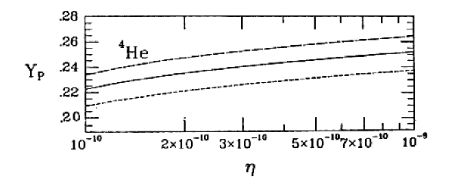
Figure 1: Predicted values for $Y_{P}$ for different values of $N_{\nu}$

Precise results for the Helium mass fraction $Y_{\rm P}$ depend on the actual value of $N_{\nu}$ and $\eta$ (as well as on the neutron lifetime, $\tau_{n}$). As we saw, $X_{n}(T^{*})$ is larger the larger $N_{\nu}$ is. Thus $Y_{\rm P}$ increases with increasing $N_{\nu}$. Similarly, a larger $\eta$ also leads to a larger $X_{n}(T_{d})$ and hence a larger $Y_{\rm P}$. Fig. 1 shows the results of a detailed calculation [10] of the primordial abundance of He, plotted as a function of $\eta$, for three different values of $N_{\nu}$ ($N_{\nu}=2,3,4$). Clearly, if one knew $\eta$, from estimates of $Y_{\rm P}$ one could infer a value for $N_{\nu}$. One way to infer $\eta$ is to compute also the primordial abundances of other light elements, besides Helium, produced by nucleosynthesis. Demanding concordance of these results fixes $\eta$ and one can then infer a value for $N_{\nu}$ from cosmology[7]. The results of the Chicago group[11] in the early 1980’s, shown in Fig. 2, using a range $0.22<Y_{\rm P}<0.26$ for the Helium abundance, predicted

$$N_{\nu}\leq 4~{}.$$ (12)

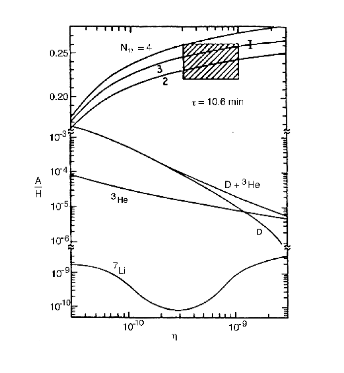
Figure 2: Primordial abundance of light elements as a function of $\eta$

This cosmological inference was verified at LEP and the SLC almost a decade later, by studying $e^{+}e^{-}$ scattering at the energy of the $Z$ boson mass. The amplitude for the annihilation of $e^{+}$ and $e^{-}$ into a fermion-antifermion pair depends on the width of the $Z$

$$A(e^{+}e^{-}\to f\bar{f})\sim\frac{1}{s-M_{Z}^{2}+i\Gamma_{Z}M_{Z}}~{}.$$ (13)

This width, in turn, depends on the number of light neutrinos species—where light here means $m_{\nu}\ll\frac{M_{Z}}{2}$. One has:

$$\Gamma_{Z}=\Gamma(Z\to\hbox{charged states})+N_{\nu}\Gamma(Z\to\nu\bar{\nu})~{}.$$ (14)

Fig. 3 plots some early data from the ALEPH[12] collaboration at LEP which clearly shows that $N_{\nu}=3$ is preferred. The most recent compilation of results from all the four LEP collaborations[13] doing a Standard Model fit, gives

$$N_{\nu}=2.993\pm 0.011~{}.$$ (15)

A less accurate, but more direct measurement of the, so-called, invisible width of the $Z$—assuming that this width is due to $Z$ decays into neutrino pairs—gives instead

$$N_{\nu}=3.09\pm 0.13~{}.$$ (16)

Thus, there is now strong evidence that $N_{\nu}=3$.

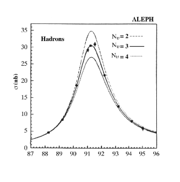
Figure 3: Plot of $\sigma(e^{+}e^{-}\rightarrow{\rm hadrons})$ at the Z-resonance

Given these results, the present-day discussions of nucleosynthesis take $N_{\nu}=3$ and try to get stronger limits on the baryon to photon ratio $\eta$ from the demand of concordance of all the primordial abundances. A recent example of such an analysis is the work of Copi, Schramm and Turner[14], whose results are depicted in Fig. 4, yielding for $\eta$ the range

$$2.4\times 10^{-10}<\eta\leq 4.2\times 10^{-10}~{}.$$ (17)

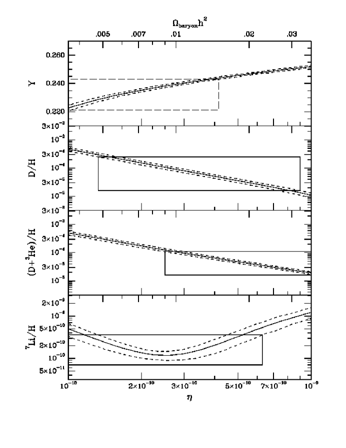
Figure 4: Concordance of meausured primordial element abundances, from [14]

A recent study of updated data for primordial ${}^{4}{\rm He}$ by Olive, Skillman and Steigman[15] pins down $Y_{\rm P}$ in a narrow range

$$Y_{\rm P}=0.234\pm 0.002\pm 0.005~{},$$ (18)

where the first error is statistical and the second is an estimate of the possible systematic error. Using the above, the 95% confidence limit for $Y_{\rm P}$ gives $Y_{\rm P}<0.244$, which allows Olive, Skillman and Steigman[15] to set a 95% CL for $\eta$ of

$$\eta<3.8\times 10^{-10}~{}~{}~{}~{}~{}~{}~{}~{}~{}(95\%~{}{\rm CL})~{}.$$ (19)

This result is in agreement with the recent work on the primordial abundance of deuterium obtained by studying quasi-stellar objects (QSO) absorption lines[16], which infers a rather high primordial deuterium abundance. However, very recent work by Tytler et al.[17], based on two correlated QSO observations, obtains a discordant, very low, primordial deterium abundance yielding large $\eta$ values:

$$5.1\times 10^{-10}<\eta<8.2\times 10^{-10}~{}.$$ (20)

Such values correspond to a range for $Y_{\rm P}$ ($0.246<Y_{\rm P}<0.282$) above the 95% limit of Olive, Skillman and Steigman[15].

Clearly, the situation at the moment is still unsettled and it is difficult to draw strong inferences. Possibly, the simplest assumption to make is that the actual value for $Y_{\rm P}$ is subject to much stronger systematic uncertainties that those assumed by Olive, Skillman and Steigman[15]. In what follows, we shall take the value obtained by Copi, Schramm and Turner[14] for $\eta$ but, following their suggestion, shall boost it to cover a $2\sigma$ range. Then one has

$$1.9\times 10^{-10}<\eta<5.8\times 10^{-10}~{}~{}~{}~{}~{}~{}~{}(2\sigma~{}\hbox{range})~{},$$ (21)

which is a range broad enough to encompass all recent determinations.

3 Two Open Problems in Cosmology: Dark Matter and Baryogenesis

The ratio $\eta$, which we just saw is important for nucleosynthesis, lies at the heart of two of the biggest open problems in cosmology today, those of dark matter and of baryogenesis. Recall that $\eta$ was the ratio of the number density of baryons to photons in the Universe now. The photon density itself is extremely well known from the measurement of the temperature of the cosmic background radiation[18]

$$T_{\gamma}=(2.726\pm 0.005)^{\circ}{\rm K}~{},$$ (22)

yielding

$$n_{\gamma}=\int\frac{q^{2}dq}{\pi^{2}}\frac{1}{(e^{q/T_{\gamma}}-1)}=[0.625~{}T_{\gamma}]^{3}\simeq 400~{}{\rm cm}^{-3}~{}.$$ (23)

Therefore a value for $\eta$ serves to fix the energy density of baryons in the Universe now:

$$\rho_{\rm B}=m_{N}n_{\rm B}=m_{N}\eta n_{\gamma}~{},$$ (24)

where $m_{N}$ is the nucleon mass. Using Eqs. (21) and (23) one finds

$$1.3\times 10^{-31}~{}{\rm g/cm}^{3}<\rho_{\rm B}<4\times 10^{-31}~{}{\rm g/cm}^{3}~{}.$$ (25)

This value is interesting since, as we shall see below, it is a few percent of what is needed to close the Universe.

If one does not neglect the curvature term, Einstein’s equations in a Friedmann Robertson Walker Universe have the form

$$H^{2}=\left(\frac{\dot{R}}{R}\right)^{2}=\frac{8\pi G_{N}}{3}\rho-\frac{k}{R^{2}}~{}.$$ (26)

The constant k here describes the geometry of the Universe. If $k>0$, the Universe is closed. If $k<0$, it is open. Finally, if $k$ vanishes, one has a Universe with no curvature—a flat Universe. It is useful to consider the quantity $\Omega(t)$, which is essentially the ratio of the matter density to the square of the Hubble parameter

$$\Omega(t)=\frac{\rho}{\left[\frac{3}{8\pi}\frac{H^{2}}{G_{N}}\right]}~{}.$$ (27)

Using Einstein’s equations, one sees that $\Omega(t)$ characterizes the geometry

$$\Omega(t)=\frac{1}{1-X(t)}~{};~{}~{}~{}~{}~{}X(t)=\frac{\left[\frac{k}{R^{2}}\right]}{\left[\frac{8\pi G_{N}}{3}\rho\right]}~{},$$ (28)

with $\Omega>1$ corresponding to a closed Universe, and $\Omega<1$ corresponding to an open Universe. The value of $\Omega(t)$ at the present time $\Omega_{o}$ depends on how $\rho$ compares to the, so-called, critical density

$$\rho_{o}=\frac{3H_{o}^{2}}{8\pi G_{N}}~{},$$ (29)

with $H_{o}$ being the value of the Hubble parameter now—the Hubble constant.

From Eq. (28) one sees that a flat Universe has $\Omega(t)=1$. Thus the ratio of the Universe’s density now to the critical density:

$$\Omega_{o}=\frac{\rho}{\rho_{o}}$$ (30)

directly informs one about the Universe’s geometry, with $\Omega_{0}=1$ corresponding to a flat Universe. Unfortunately, the Hubble constant itself is not that easily determined. Conventionally, one writes:

$$H_{o}=100~{}{\rm h}\frac{{\rm Km}}{\rm{Mpc~{}sec}}~{},$$ (31)

and one typifies the uncertainty in $H_{o}$ through a range for h. Traditionally, this uncertainty corresponds to h lying in the range

$$0.5<{\rm h}<1~{},$$ (32)

although a more modern determination[19] gives

$$h=0.6\pm 0.1~{}.$$ (33)

Numerically, one finds that the critical density has the value

$$\rho_{o}=1.9\times 10^{-29}~{}{\rm h}^{2}~{}{\rm g/cm}^{3}~{}.$$ (34)

If the density of the Universe is above $\rho_{o}$ the Universe is closed. Clearly, if baryons dominate the energy density of the Universe, Eq. (25) tells us that the Universe is open.

If we denote the baryonic contribution to $\Omega_{o}$ by $\Omega_{\rm B}=\rho_{\rm B}/\rho_{o}$, using Eq. (25) and (34), one has[14]

$$0.007\leq\Omega_{\rm B}{\rm h}^{2}\leq 0.021~{}.$$ (35)

This equation is remarkable in several ways. First, it appears that $\Omega_{\rm B}$ itself is much bigger than the value one would infer from the amount of luminous matter in the Universe. Using h = $0.6\pm 0.1$, from Eq. (35) one sees that $\Omega_{\rm B}$ ranges from about 0.014 to 0.084. On the other hand, the best estimates of the fraction of luminous matter in the Universe[20] give a range

$$\Omega_{\rm luminous}\simeq 0.003-0.017~{},$$ (36)

half an order of magnitude smaller. So one infers that there is substantial non-luminous baryonic dark matter. The existence of this dark matter is also inferred from the observed flat rotation curves in spiral galaxies. Normally, outside the luminous body of the galaxy, one would expect the circular velocity to drop as $r^{-1/2}$, but it does not, as shown in Fig. 5. From these measurements, one deduces values[21]

$$\Omega_{\rm rot.~{}curves}\simeq 0.03-0.10~{},$$ (37)

much more comparable to those for $\Omega_{\rm B}$.

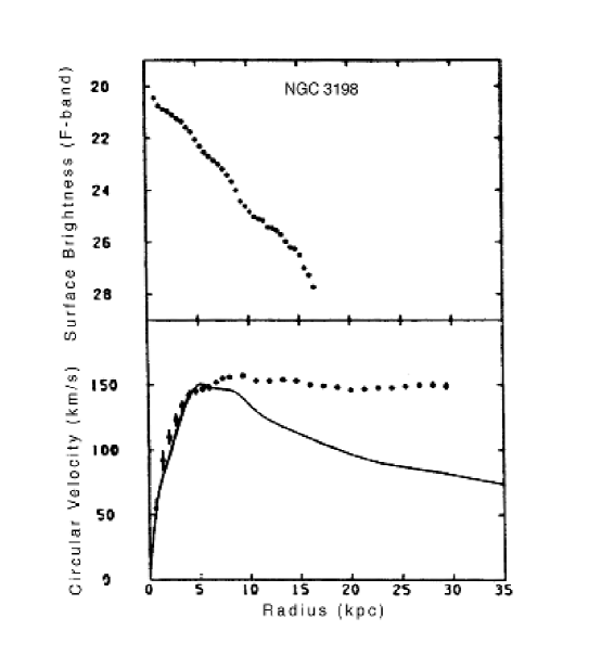
Figure 5: A typical flat rotation curve extending beyond the luminous body of the galaxy

Second, since $\Omega_{\rm B}$ is much bigger than the contribution to the energy density made by photons, neutrinos and electrons, if $\Omega_{o}\simeq\Omega_{\rm B}$ then there is an enormous fine-tuning problem. In this case, the parameter $X(t)$ now, $X_{o}$, is roughly of order ten to one hundred:

$$X_{o}=1-\frac{1}{\Omega_{o}}\simeq-\frac{1}{\Omega_{\rm B}}~{}.$$ (38)

However, $X(t)$ being the ratio of the curvature term to the energy density term [cf. Eq. (28)] scales as $X(t)\sim R^{2}(t)\sim T^{-2}$. Hence $X(t)\simeq-1/\Omega_{\rm B}~{}(T_{o}/T)^{2}$ and therefore

$$\Omega(T)\simeq\frac{1}{1+\frac{1}{\Omega_{\rm B}}\left(\frac{T_{o}}{T}\right)^{2}}~{}.$$ (39)

To get $\Omega_{o}\simeq\Omega_{\rm B}$ now, in the early Universe the density must have been unbelievably close to the critical density. For instance at the Planck temperature, $T_{\rm P}\simeq 10^{32}~{}^{\circ}{\rm K}$, $\Omega(T_{\rm P})\simeq 1-~{}O(10^{-62})$ !

The solution to the fine-tuning problem above is provided by inflation.[3] In an inflationary Universe, there is an exponential growth of the scale factor at early times. Effectively then the curvature term ${\rm k}/R^{2}$ is totally negligible and the latter evolution of the Universe corresponds to that of a flat Universe, with ${\rm k}_{\rm eff}=0$. Thus, if one wants to avoid fine-tuning as a result of inflation, then $\Omega(t)=1$ and the Universe is always at the critical density. In this case, the value of $\Omega_{\rm B}$ obtained, since it is in the percent range, tells us that the Universe is dominated by non-baryonic dark matter.

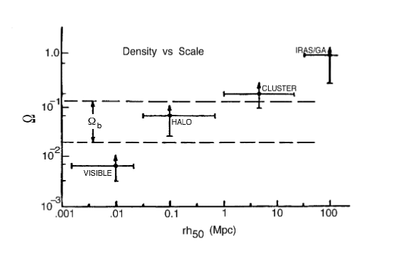
Figure 6: Variation in $\Omega_{0}$ as a function of the scale of the structures meausured

Besides the theoretical bias for considering $\Omega=1$, there is actually observational evidence for $\Omega$ being greater than $\Omega_{\rm B}$, obtained by reconstructing the energy density from the flow of peculiar velocities in superclusters of galaxies. It appears that the values of $\Omega_{o}$ one infers are largest when one measures the density on the largest structures in the Universe, as shown in Fig. 6. All the data on $\Omega_{o}$ has been summarized recently by Dekel, Burnstein and White[22] who, if one assumes that there is no cosmological constant, give the following range for this quantity:

$$0.3\leq\Omega_{o}\leq 1.3~{}.$$ (40)

The lower bound above comes from the cosmic velocity flows, while the upper bound comes from the age of the Universe (assuming h = $0.6\pm 0.1$). Fig. 7 summarizes these results, allowing for the possibility of a cosmological constant.

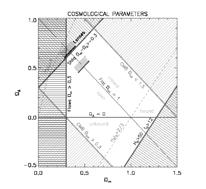
Figure 7: Summary of present status of $\Omega_{0}$, from [22]

Very recent data on type-I supernovas at high redshift [23] [24] has provided some evidence, at the 3$\sigma$ level, that the Universe’s expansion is actually accelerating rather than decelerating. Since the deceleration parameter[25] meausures the difference between the contribution of matter to $\Omega$ and that of the cosmological constant

$$q^{0}=\frac{\Omega_{M}}{2}-\Omega_{\Lambda},$$ (41)

this data suggests a non vanishing cosmological constant. However, these results are based on the assumption that supernovas are standard candles. Further, they are critically dependent on the highest redshift supernovas observed. There is also some disagreement among the results of the two groups. For a flat Universe, [23] obtains $\Omega_{M}=0.32\pm 0.1$ and $\Omega_{\Lambda}=0.68\pm 0.1$, while [24] find $\Omega_{M}=0.6\pm 0.2$ and $\Omega_{\Lambda}=0.4\pm 0.2$. In my view, it is probably to early to abandon the idea of a Universe where only matter (of all types) contributes to give $\Omega=1$. However, these results give one pause.

The parameter $\eta$, besides fixing $\Omega_{\rm B}$ and adumbrating the dark matter problem, has another role. $\eta$ is also a measure of the amount of matter-antimatter asymmetry in the Universe. From observation, it appears that the Universe is matter dominated, with little or no antimatter.[26] The observed antiprotons in cosmic rays, whose typical ratio to protons is of $O(\bar{p}/p\sim 10^{-4})$, are entirely consistent with the flux coming from pair production. Furthermore, no characteristic $\gamma$-rays are seen in the sky which could arise from $p-\bar{p}$ annihilations. If the Universe had islands of antimatter, one would expect such signals to be present. In addition, there are also theoretical difficulties in assuming that the Universe was matter-antimatter symmetric in its late evolution. In this case, one can estimate the amount of matter that would remain after the $p$ and $\bar{p}$ in the Universe go out of equilibrium around $T\sim O(1~{}{\rm GeV})$. Below this temperature inverse annihilations ($2\gamma\to p+\bar{p}$) are blocked and the direct process $p+\bar{p}\to 2\gamma$ considerably reduces the number of protons (and antiprotons) compared to that of photons to values of $\eta\sim 10^{-18}$[6].

For these reasons, $\eta\sim O(10^{-10})$, as observed, is evidence that there was some primordial baryon asymmetry. That is, really,

$$\eta=\frac{(n_{\rm B}-n_{\bar{\rm B}})}{n_{\gamma}}~{}.$$ (42)

If the value of $\eta$ were to codify an initial asymmetry for the Universe, this would appear to be a pretty mysterious initial condition. Fortunately, as Sakharov[1] first pointed out, it is possible to generate such a baryon-antibaryon asymmetry dynamically and so $\eta$ can be a reflection of some primordial processes. To generate such an asymmetry dynamically, as we will discuss later on in much greater detail, the underlying theory must violate baryon number, as well as C and CP. Thus it appears that even though $\eta$ is an important cosmological parameter, its origins are tied to particle physics also!

4 Hot and Cold Dark Matter

An important classification scheme for dark matter is whether the relic dark matter candidates were created by a thermal process or as a result of some non-thermal process (e.g. in a phase transition). Thermal relics can be further distinguished by whether they were relativistic or non-relativistic at the time their interaction rate fell below the Universe’s expansion rate. Relics which were relativistic at freeze-out are labeled hot dark matter (HDM), while relics which were non-relativistic at freeze-out are called cold dark matter (CDM).

Particle physics provides possible dark matter candidates in all these categories. Neutrinos, neutralinos and gravitinos are thermal relics, while axions are an example of a non-thermal relic. Neutrinos are a prototypical hot dark matter relic. Neutralinos are an example of cold dark matter, while gravitinos are warm dark matter candidates. Because only zero momentum axions can contribute substantially to the Universe’s energy density, axions are also cold dark matter candidates. In what follows, I will describe some of the characteristics of these possible dark matter candidates.

The contribution of thermal relics to $\Omega$ depends on what their abundance was when their interaction rate fell below the Universe’s expansion rate. Freeze-out occurs when, for the relic $\chi$, $\Gamma_{\chi}\simeq H$. For hot relics the freeze-out temperature is much greater than the mass of the relic: $T_{\chi}\gg m_{\chi}$. In this case, at freeze-out $n_{\chi}\sim n_{\gamma}$. Because the density of the relic to that of photons is an invariant, the contribution to $\Omega_{0}$ of any hot dark matter relic is just a function of its mass (and $T_{\gamma}^{0}\simeq 3^{\circ}{\rm K}$). Calling this contribution $\Omega_{\chi}$, one finds

$$\Omega_{\chi}[{\rm HDM}]=\frac{m_{\chi}n_{\chi}^{0}}{\rho_{0}}\simeq\frac{m_{\chi}n_{\gamma}^{0}}{g^{*}\rho_{0}}\simeq\frac{1}{g^{*}}\left[\frac{m_{\chi}}{92~{}{\rm eV}}\right]\frac{1}{h^{2}}~{}.$$ (43)

Here $g^{*}$ counts the effective degrees of freedom at freeze-out, with $g^{*}=1$ for neutrinos. The above shows that particles with eV masses can be cosmologically significant, contributing substantially to the Universe’s energy density. This observation was first made about 25 years ago by Cowsik and McClelland[27] and Marx and Szalay[28] with regards to neutrinos.

Cold relics, on the other hand, undergo freeze-out at temperatures much less than their mass: $T_{\chi}\ll m_{\chi}$. In this case their density is suppressed relative to the photon density by a Boltzmann factor, so that at freeze-out $n_{\chi}\ll n_{\gamma}$. This density, however, can be deduced from the freeze-out condition itself

$$\Gamma_{\chi}=n_{\chi}\langle\sigma v\rangle_{\chi}\biggr{|}_{\hbox{freeze-out}}=H\simeq 1.7(g^{*})^{1/2}T_{\chi}^{2}/M_{\rm P}~{},$$ (44)

where $g^{*}$ is the effective number of degrees of freedom at freeze-out and $\langle\sigma v\rangle_{\chi}$ is the, thermally-averaged, annihilation rate for the cold dark matter relic $\chi$. In this case, the contribution to $\Omega_{0}$ of the relic depends both on this annihilation rate and on the ratio $m_{\chi}/T_{\chi}$. One finds, approximately,[6]

$$\Omega_{\chi}[{\rm CDM}]\simeq\frac{m_{\chi}}{T_{\chi}}\left[\frac{10^{-27}{\rm cm}^{3}/{\rm sec}}{\langle\sigma v\rangle_{\chi}\big{|}_{\hbox{freeze-out}}}\right]~{},$$ (45)

a formula first deduced by Zeldovich[29]. For a typical ratio $m_{\chi}/T_{\chi}\sim 20$ one needs cross sections of $O(\sigma\sim 10^{-36}~{}{\rm cm}^{2})$. These cross sections are of the typical strength of weak interaction processes. It is clearly intriguing that such cross sections could have cosmological significance!

There are no simple formulas to describe the contributions to $\Omega$ of non-thermal relics, since these contributions depend in detail on the dynamics. In general, for non-thermal relics, the interactions are so feeble that one has always $\Gamma_{\chi}\ll H$; that is, the relics are never in thermal equilibrium. For example, as we shall see later on, axions with $m_{a}\simeq 10^{-5}~{}{\rm eV}$ can close the Universe $(\Omega_{\rm axions}\simeq 1)$. This means that the number density of axions in this case is about $10^{7}$ times what it would be if axions were thermal relics (i.e. had a $3^{\circ}~{}{\rm K}$ temperature). So, if axions are the dark matter in the Universe, they obviously had a highly non-thermal origin.

5 Prospects of Neutrinos as Dark Matter

Neutrinos are interesting candidates for dark matter since their properties fit the required profile. Furthermore, neutrinos are the only dark matter candidates whose existence is confirmed experimentally! Originally, neutrinos were thought to provide possible examples for both hot dark matter and cold dark matter. Because of LEP, we know now that they can only be HDM candidates. Let me elaborate on this point.

Experimentally, one has evidence that the three known neutrinos, $\nu_{e},\nu_{\mu}$, and $\nu_{\tau}$, are quite light, with direct bounds on their masses given by[30]

$$m_{\nu_{e}}\leq 15~{}{\rm eV}~{};~{}~{}~{}~{}m_{\nu_{\mu}}\leq 170~{}{\rm keV}~{};~{}~{}~{}~{}m_{\nu_{\tau}}\leq 24~{}{\rm MeV}~{}.$$ (46)

Because the freeze-out temperature for neutrinos is of order of $T_{f}\sim 1~{}{\rm MeV}$, so as not to overclose the Universe $\nu_{\mu}$ and $\nu_{\tau}$ must have masses much below these bounds. Hence, it is perfectly conceivable that the known neutrinos are the hot dark matter, contributing to $\Omega_{0}$ an amount

$$\Omega_{\nu}=\left[\frac{\sum_{i}m_{\nu_{i}}}{92~{}{\rm eV}}\right]\frac{1}{h^{2}}~{}.$$ (47)

If heavy neutrinos existed, with masses $m_{\nu_{H}}\gg T_{f}\sim 1~{}{\rm MeV}$, they could be cold dark matter candidates because they have weak interactions. It is straightforward, knowing the interaction rate of neutrinos, to calculate their contribution to $\Omega$ as a function of the neutrino mass. The result is displayed in Fig. 8, taken from[6]. This figure shows that $\Omega_{\nu}$ grows with $m_{\nu}$ up to around the freeze-out temperature $T_{f}$ and then decreases rather rapidly for neutrino masses beyond this temperature. However, the existence of further neutrino species with $m_{\nu}\leq\frac{1}{2}M_{Z}$ is now excluded by measurements of the $Z$-width at LEP, which, as we saw earlier, gives $N_{\nu}=3$ to high accuracy. Thus the window for heavy neutrino CDM is closed.

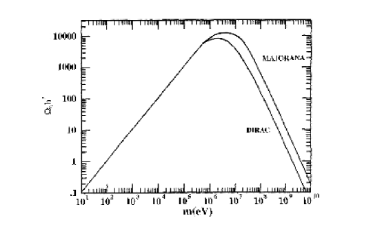
Figure 8: Contribution of neutrinos of different masses to $\Omega h^{2}$, from [6]

Although neutrinos are not cold dark matter candidates, they remain excellent prospects for hot dark matter. Nevertheless, because one knows that hot dark matter alone cannot describe the power spectrum of density fluctuations[31], one expects $\Omega_{\nu}<1$. Acceptable fits to the power spectrum of density fluctuations suggest typically[31] $\Omega_{\nu}\simeq 0.2$. Using $h^{2}\simeq 0.3$, if neutrinos are the HDM, this gives

$$\sum m_{\nu_{i}}\simeq 5-6~{}{\rm eV}~{}.$$ (48)

This ratio is consistent with the bounds[30] given in Eq. (46). Unfortunately, however, there is as yet no direct particle physics evidence that the known neutrinos have masses that satisfy Eq. (48). Nevertheless, there is tantalizing indirect evidence for neutrino masses (through hints of neutrino oscillations) and this evidence is compatible with Eq. (48). Because of its importance to the issue at hand, I review next some of this information and its implications.

First, let me make a comment on prospects for improving the direct neutrino mass bounds quoted in[30]. Clearly, even though the kinematical techniques that give the bounds on $m_{\nu_{\mu}}$ and $m_{\nu_{\tau}}$ can perhaps be improved somewhat, there is no hope to directly measure masses in the few eV range for these particles. This is not so for $\nu_{e}$. In fact, the tritium $\beta$-decay experiments that lead to the bound of $m_{\nu_{e}}\leq 15~{}{\rm eV}$ quoted by the Particle Data Group[30], actually all have sensitivities of order 1-2 eV! The reason for the much weaker bound quoted, is that all the latest precision experiments[32] are plagued by an anomalous unexplained excess of events beyond the tritium beta decay endpoint. This excess actually leads to an average mass-squared that is negative ($\langle m_{\nu_{e}}^{2}\rangle=(-27\pm 20)~{}{\rm eV}^{2})$.[30] Until this excess is understood, one cannot set a real bound for $m_{\nu_{e}}$, although the potential sensitivity to eV masses is there.

In this context, one should mention a different piece of evidence that suggests that $\nu_{e}$ itself cannot be the dominant form of the HDM. This latter constraint comes from double-beta decay, where searches for the neutrinoless mode in ${}^{76}{\rm Ge}$ decay[33] lead to a limit on the effective neutrino Majorana mass responsible for this process of

$$\langle m_{\nu}\rangle_{ee}\leq(0.5-1.5)~{}{\rm eV}~{}.$$ (49)

Here $\langle m_{\nu}\rangle_{ee}$ is the sum of the neutrino masses entering in the process, convoluted with the appropriate mixing matrix element coupling these neutrinos (and antineutrinos) to electrons:

$$\langle m_{\nu}\rangle_{ee}=\sum_{i}U^{2}_{ei}m_{i}~{}.$$ (50)

If mixing of electrons to neutrinos other than $\nu_{e}$ is not large $(U_{e1}\simeq 1)$, then Eq. (49) is also a bound on $m_{\nu_{e}}$. However, this is not a true bound because if neutrinos are Dirac particles, the particle and antiparticle contributions in Eq. (50) automatically cancel and $\langle m_{\nu}\rangle_{ee}\equiv 0$.

Fortunately, one can probe neutrino masses indirectly by looking for evidence for oscillations of one neutrino species into another. If neutrinos have mass, neutrinos can mix with one another and this mixing can be revealed through neutrino oscillation experiments. At present there are a number of tantalizing hints arising from experiments looking for neutrino oscillations which have an important bearing on the question of neutrino mass. To discuss these experiments, it is necessary first to briefly discuss a bit of phenomenology.

If neutrinos have mass, the weak interaction eigenstates (the neutrinos produced by weak interaction processes–e.g. $W^{+}\to e^{+}\nu_{e}$), are not the same as the mass eigenstates (i.e. the observed particles of well defined mass, denoted here by $\nu_{i}$). However, these states are related by a unitary transformation, so that each $\nu_{\ell}~{}\{\ell=e,\mu,\tau\}$ can be written as a superposition of the $\nu_{i}$:

$$\nu_{\ell}=\sum_{i}U_{\ell i}\nu_{i}~{}.$$ (51)

Conventionally, one only examines the $2\times 2$ case, assuming that, as in the quark case, the $3\times 3$ matrix will be nearly diagonal with dominant mixing among pairs of neutrinos. In this case, for instance, Eq. (51) for $\nu_{e}$ and $\nu_{\mu}$ just involves a simple orthogonal $2\times 2$ matrix:

$$\left(\begin{array}[]{c}\nu_{e}\\ \nu_{\mu}\end{array}\right)=\left(\begin{array}[]{cc}\cos\theta&\sin\theta\\ -\sin\theta&\cos\theta\end{array}\right)\left(\begin{array}[]{c}\nu_{1}\\ \nu_{2}\end{array}\right)~{}.$$ (52)

The mass eigenstates $\nu_{i}$ have the usual quantum mechanical evolution with time:

$$|\nu_{i}(t)\rangle=e^{-iE_{i}t}|\nu_{i}(0)\rangle~{}.$$ (53)

Imagine then producing at $t=0$ a $\nu_{e}$ from a weak decay

$$|\nu(0)\rangle\equiv|\nu_{e}\rangle=\cos\theta|\nu_{1}(0)\rangle+\sin\theta|\nu_{2}(0)\rangle~{}.$$ (54)

At a later time, because the states $\nu_{1}$ and $\nu_{2}$ have different masses, this state will evolve into a superposition of both $|\nu_{e}\rangle$ and $|\nu_{\mu}\rangle=-\sin\theta|\nu_{1}(0)\rangle+\cos\theta|\nu_{2}(0)\rangle$. That is

$$|\nu(t)\rangle = \cos\theta|\nu_{1}(t)\rangle+\sin\theta|\nu_{2}(t)\rangle$$ (55)

$$= \cos\theta e^{-iE_{1}t}|\nu_{1}(0)\rangle+\sin\theta e^{-iE_{2}t}|\nu_{2}(0)\rangle~{}.$$

Using the above, it is easy to calculate the transition probability that an initial $\nu_{e}$ state has oscillated into a $\nu_{\mu}$ state after a time $t$:

$$P(\nu_{e}\to\nu_{\mu};t) = |\langle\nu(t)|\nu_{\mu}\rangle|^{2}$$ (56)

$$= \frac{1}{2}\sin^{2}2\theta[1-\cos(E_{1}-E_{2})t]~{}.$$

In all cases of interest $|p|\gg m_{i}$. Hence $E_{i}\simeq|p|+\frac{m_{t}^{2}}{2|p|}$, with $|p|\equiv E_{\nu}$ being essentially the neutrino energy. Also, in this case, the time $t$ in Eq. (56) can just be replaced by the distance travelled (in units of the speed of light): $t=L/[c]$. Whence, one finds the following formula for the probability that, as a result of neutrino mixing, an initial $\nu_{e}$ of energy $E_{\nu}$ has oscillated after a distance $L$ into a $\nu_{\mu}$:

$$P(\nu_{e}\to\nu_{\mu};L) = \sin^{2}2\theta\sin^{2}\left[\frac{(m_{1}^{2}-m_{2}^{2})L}{4E_{\nu}}\right]$$ (57)

$$= \sin^{2}2\theta\sin^{2}\left[1.27\frac{\Delta m^{2}({\rm eV})L(m)}{E_{\nu}({\rm MeV})}\right]~{}.$$

Of course,

$$P(\nu_{e}\to\nu_{e};L)=1-P(\nu_{e}\to\nu_{\mu};L)~{}.$$ (58)

One sees from the above formulas that the probability of oscillation is sensitive to the mixing angle $\theta$. Further, if one wants to probe a particular $\Delta m^{2}$ range, then for a given neutrino energy $E_{\nu}$ there are appropriate distances $L$ where the effect is maximum. If the neutrinos are not nearly degenerate, then the $\Delta m^{2}$ range one wants to probe to find out whether neutrinos contribute significantly to the dark matter problem (cosmologically significant neutrinos) is $\Delta m^{2}\sim 25~{}{\rm eV}^{2}$. This is the goal of the CHORUS and NOMAD experiments at CERN, which for $\Delta m^{2}$ in this range hope to be sensitive to $\nu_{\mu}\to\nu_{\tau}$ oscillations as low as $\sin^{2}2\theta_{\mu\tau}\geq 10^{-3}$.

Up to now the CERN experiments have only given limits.[34] However, in other regions of $\Delta m^{2}$ there are various hints of neutrino oscillations. In fact, there is an embarrassment of riches! The LSND experiment[35] sees a signal of $\bar{\nu}_{\mu}\to\bar{\nu}_{e}$ oscillations in a narrow range in $\Delta m^{2}$ around (0.2-2) ${\rm eV}^{2}$, with $\sin^{2}2\theta\simeq 10^{-2}~{}{\rm eV}^{2}$. The ratio of $\nu_{\mu}$ to $\nu_{e}$ neutrinos, observed in large underground experiments, arising from decay processes in the atmosphere shows a deficit[36] from what is expected. This atmospheric anomaly can be interpreted either as being due to $\nu_{\mu}\to\nu_{\tau}$ or $\nu_{\mu}\to\nu_{e}$ oscillations, with $\Delta m^{2}\sim(0.3-3)\times 10^{-2}~{}{\rm eV}^{2}$ and large mixing angles $\sin^{2}2\theta\simeq O(1)$. Finally, experiments measuring the flux of solar neutrinos, also show a dearth of neutrinos compared to the predictions of the, so called, standard solar model.[39] One can reconcile the observations of all of these solar neutrino experiments by appealing to $\nu_{e}\to\nu_{\mu}$ or $\nu_{e}\to\nu_{\tau}$ neutrino oscillations, which are enhanced in matter by the so-called MSW mechanism,[40] provided that $\Delta m^{2}\sim(0.3-1.2)\times 10^{-5}~{}{\rm eV}^{2}$ with rather small mixing: $\sin^{2}2\theta\sim(4-10)\times 10^{-3}$.[41]

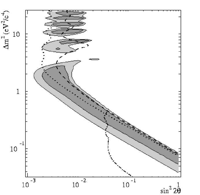
Figure 9: Signal region for the LSND experiment, along with exclusion limits from other experiments [35]

Because we know of only three neutrino species, these hints cannot all be true, since we have at most only two mass differences! Even if one were to eliminate one of the hints (LSND perhaps–since, as Fig. 9 make clear, the allowed region is almost ruled out by other negative findings), because the favored mass differences are small, it appears that to have cosmologically significant neutrinos one must have near mass degeneracy. For example, the pattern $m_{\nu_{1}}\simeq m_{\nu_{2}}\simeq m_{\nu_{3}}\simeq 1-2~{}{\rm eV}$, with $\Delta m^{2}_{12}\sim 10^{-5}~{}{\rm eV}^{2}$; $\Delta m^{2}_{23}\sim 10^{-3}~{}{\rm eV}^{2}$ would explain the solar and atmospheric anomaly. If this were really the case, then cosmologically significant neutrinos would produce no signal in CHORUS and NOMAD! Hopefully, in the next five years with upcoming neutrino oscillation experiments (as well, perhaps, with some clarification in the direct tritium $\beta$-decay experiments) one should be able to sort out this somewhat confusing situation, thereby arriving at a better understanding of whether or not neutrinos can contribute to the dark matter in the Universe.

Before closing this section, I would like to make an important theoretical point. Neutrino masses in the eV and sub-eV ranges are very interesting from a particle physics point of view, since they are most likely a signal for a new large mass scale. In general, because neutrinos are neutral, they can have both Dirac - particle/anti-particle—and Majorana - particle/particle masses. That is, one can write

$${\cal{L}}_{\rm mass}=-m_{D}\bar{\nu}_{\rm L}\nu_{\rm R}-\frac{1}{2}m^{\rm R}_{M}\nu^{T}_{\rm R}C\nu_{\rm R}-\frac{1}{2}m^{\rm L}_{M}\nu^{T}_{\rm L}C\nu_{\rm L}+h.c.~{},$$ (59)

where $C$ is a charge conjugation matrix.[44] Because $\nu_{\rm L}$ is part of an SU(2) doublet, while $\nu_{\rm R}$ (if it exists!) is part of an SU(2) singlet, it is clear that in the standard model $m_{M}^{\rm R},m_{D}$ and $m_{M}^{\rm L}$, respectively, carry effective SU(2) quantum numbers of 0, 1/2 and 1. In particular, while $m_{M}^{\rm R}$ can be a totally independent mass parameter, $m_{D}$ and $m_{M}^{\rm L}$ must be proportional to the vacuum expectation value of an SU(2) doublet and triplet field, respectively. We know, as a result of the experimentally very successful interrelation between $M_{W}$ and $M_{Z}$: $M_{Z}^{2}\cos^{2}\theta_{W}=M^{2}_{W}$, that what causes the breakdown of the electroweak theory through its VEV transforms dominantly as an SU(2) doublet. Thus, if $\nu_{\rm R}$ exists, we expect $m_{M}^{\rm L}\ll m_{D}$, with $m_{D}\sim m_{\ell}$—the mass of the corresponding lepton.

It was realized long ago by Yanagida[45] and Gell-Mann, Ramond and Slansky,[46] that if the Majorana mass of the right-handed neutrinos $m_{M}^{\rm R}$ is very large, $m_{M}^{\rm R}\gg m_{D}$, the above scenario produces very tiny neutrino masses. If one neglects altogether $m_{M}^{L}$, $m_{M}^{L}\simeq 0$, one has a $2\times 2$ neutrino mass matrix of the form

$${\cal{M}}=\left(\begin{array}[]{cc}0&m_{D}\\ m_{D}&m_{M}^{\rm R}\end{array}\right)~{}.$$ (60)

This matrix has a very heavy neutrino, mostly $\nu_{\rm R}$, with mass $m_{M}^{\rm R}$ and a very light neutrino, mostly $\nu_{\rm L}$, with mass

$$m_{\nu}\simeq\frac{m_{D}^{2}}{m_{M}^{\rm R}}\sim\frac{m_{\ell}^{2}}{m_{M}^{\rm R}}~{}.$$ (61)

This, so-called, see-saw mechanism [45] can produce eV neutrino masses provided $m_{M}^{\rm R}$ is sufficiently large (e.g. for $m_{\nu_{\tau}}$ one has eV neutrinos associated with the tau if $m_{M}^{\rm R}\sim 10^{10}~{}{\rm GeV}!$). Thus detecting light neutrino masses is tantamount to discovering a large scale—the scale responsible for the right-handed neutrino Majorana mass.

6 Supersymmetric Candidates for Dark Matter

Supersymmetric extensions of the Standard Model for the strong and electroweak interactions provide excellent candidates for cold dark matter. Supersymmetry, as is well known[48], is a fermion-boson symmetry. Thus, if it were a true symmetry of nature, we would expect a doubling of all the degrees of freedom. Thus, in these extensions of the Standard Model, there is a plethora of undiscovered particles. Some of these particles turn out to be good dark matter candidates. This is plausible because a supersymmetric extension of the standard model preserves the strength of the couplings. For instance, the supersymmetric vertex joining a squark (the scalar partner of the quark), a quark and a gaugino (the spin-1/2 partner of a gauge boson) has the same strength as the quark-quark-gauge boson vertex. As a result, (some) of the interaction cross sections for supersymmetric (SUSY) particles will have the strength of the weak interactions (provided these particles are not much heavier than the weak bosons) and thus will satisfy Zeldovich’s criteria for cold relics, Eq. (45).

Most supersymmetric extensions considered contain a discrete symmetry, called $R$-parity:

$$R=(-1)^{3{\rm B+L}+2S}~{},$$ (62)

which is +1 for particles and -1 for sparticles. If $R$ parity is conserved, then the lightest supersymmetric particle, the LSP, by necessity is stable. If it is neutral, as is usually assumed to be the case to avoid cosmological difficulties associated with their luminosity,[49] the LSP provides an excellent candidate for cold dark matter.

We know that if supersymmetry exists it must be broken in nature. Otherwise, the masses of the supersymmetric partners, $\tilde{m}$, would be the same as that of the ordinary particles, $m$, in gross contradiction with experiment. However, we do not know really how supersymmetry breaks down. As a result, which particle is the LSP is model dependent. Nevertheless, one can make some general observations.

There are three important scales associated with SUSY breaking. The first of these is, obviously, the masses of the sparticles themselves, $\tilde{m}$. The second is the scale, $\Lambda$, which is associated with the spontaneous breaking of supersymmetry. This is assumed to occur in a, so called, hidden sector, separated from the ordinary interactions of particles. The last scale, $M$, is the scale associated with whatever phenomena acts as the messenger connecting the hidden sector with ordinary matter. This connection is shown pictorially in Fig. 10. Both $\Lambda$ and $M$ are model dependent, but one expects the masses of the sparticles to be of order

$$\tilde{m}\sim\frac{\Lambda^{2}}{M}~{}.$$ (63)

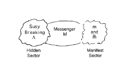
Figure 10: Scales associated with SUSY breaking

It is an attractive possibility that supersymmetry resolves the naturalness problem of electroweak symmetry breaking, related to why the scale of electroweak breaking $v\sim 250~{}{\rm GeV}$ is so much less than the Planck mass. For this to be the case, SUSY states cannot themselves have masses much bigger than $v$. Hence, it is generally assumed that supersymmetric partners must themselves be of mass $\tilde{m}\sim v$.[50] Thus $\Lambda$ and $M$, the parameters associated with supersymmetry breaking, are constrained physically to produce $\Lambda^{2}/M\sim v$.

With this constraint in mind, two main scenarios have emerged, with each scenario producing a different LSP. The first scenario arises out of supergravity models,[51] where the hidden sector is connected to the ordinary sector by gravitational interactions. Here $M\sim M_{\rm P}$ and thus $\Lambda\sim 10^{11}~{}{\rm GeV}$. In the second scenario[52] the messenger sector is associated with gauge interactions with a scale around $M\sim 10^{6}~{}{\rm TeV}$. To get $\Lambda^{2}/M\sim v$ necessitates then a much lower scale $\Lambda$ of spontaneous supersymmetry breaking, $\Lambda\sim 10^{3}~{}{\rm TeV}$.

In both scenarios the gravitino, the spin-3/2 supersymmetric partner of the graviton, becomes massive as a result of the spontaneous breaking of supersymmetry, with a mass of order

$$m_{3/2}\sim\frac{\Lambda^{2}}{M_{\rm P}}~{}.$$ (64)

From the above, one sees that in the supergravity scenario, the gravitino mass is also of $O(v)$—typical of all the other masses of the supersymmetric partners. Thus, in this case, it is generally assumed that the gravitino is not the LSP, but that the LSP is a neutralino. This is the lightest spin-1/2 partner of the neutral bosonic particles in the theory—the two gauge bosons, $\gamma$ and $Z$, and the two neutral Higgs bosons $H_{\rm u}$ and $H_{\rm d}$. In general, the neutralino is some particular superposition of all these spin-1/2 partners

$$\chi=a_{\gamma}\tilde{\gamma}+a_{Z}\tilde{Z}+a_{\rm u}\tilde{H}_{\rm u}+a_{\rm d}\tilde{H}_{\rm d}~{},$$ (65)

where the $a_{i}$ are model dependent coefficients. In contrast, in the scenario where the messenger are gauge interactions, with $M\sim 10^{6}~{}{\rm TeV}$ and $\Lambda\sim 10^{3}~{}{\rm TeV}$, the gravitino is extraordinarily light,

$$m_{3/2}\sim\frac{\Lambda^{2}}{M_{\rm P}}\sim O({\rm KeV})\ll\tilde{m}~{},$$ (66)

and is the LSP. While neutralinos, with $m_{\chi}\sim O(10-10^{3}~{}{\rm GeV})$, are typical cold dark matter relics, gravitinos, with $m_{3/2}\sim O({\rm KeV})$, act as warm dark matter. I discuss both of these cases, in turn.

The typical supergravity model[51] which gives neutralino CDM is characterized by a set of universal soft supersymmetry breaking parameters, specified at the scale $\Lambda$. In addition, it contains as a parameter the vacuum expectation ratio between the $H_{\rm u}$ and $H_{\rm d}$ Higgs bosons: $\tan\beta=\langle H_{\rm u}\rangle/\langle H_{\rm d}\rangle$. The, so called, minimal supersymmetric standard model (MSSM)[53] has actually only 2 additional parameters, besides $\tan\beta$, which determine the LSP mass, $m_{\chi}$, and the coefficients $a_{i}$ in Eq. (65). These are the common mass, $m_{1/2}$, of all the gauginos and a mass parameter $\mu$ characterizing the supersymmetric coupling between the $H_{\rm u}$ and $H_{\rm d}$ supermultiplets. However, even in this minimal model, the actual contribution of the neutralino LSP to $\Omega_{\rm CDM}$ depends on the neutralino annihilation cross sections. These, in turn, depend on other model parameters, the universal soft breaking mass $m_{o}$ given to all the scalars and certain coefficients ($A$ and $B$) which typify the strength of trilinear and bilinear soft interaction terms.[53]

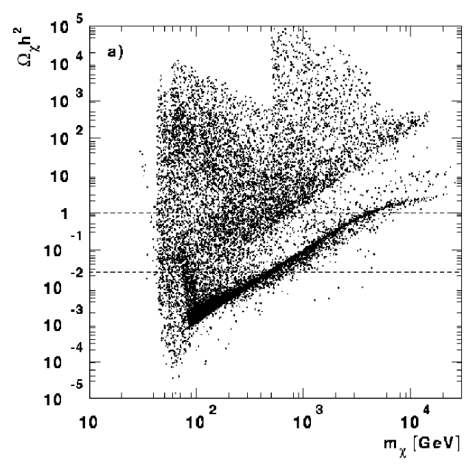
Figure 11: Contribution to $\Omega_{\chi}$ of various neutralino LSP models, from [55]

As a result, even in the MSSM, there is a large region of parameter space which produces a neutralino LSP which potentially could be the cold dark matter in the universe. Typically, what one requires for a viable model is that $\Omega_{\chi}h^{2}=0.2\pm 0.1$. As can be seen in Fig. 11, there are plenty of models (each represented by a dot) which have $50~{}{\rm GeV}\leq m_{\chi}\leq 200~{}{\rm GeV}$ and lead to $\Omega_{\chi}h^{2}$ in the desired range, provided that $\tan\beta$ is small and the resulting pseudoscalar Higgs mass $m_{A}$ is large ($m_{A}\sim 500~{}{\rm GeV}$).[54] [55] In general, an LSP much below about 50 GeV runs into trouble with the negative results from LEP on Higgs searches, as well as on the direct production of supersymmetric pairs.[56] Thus there are regions in parameter space that are already excluded, serving to rule out some potential CDM models. Clearly the discovery of an LSP would have an enormous impact on the CDM question, much reducing the parameter freedom one still has now, even for the simplest models.

In gauge mediated supersymmetry breaking models, in contrast, the gravitino is the LSP. Here one has much less freedom since there are not that many parameters to vary. Gravitino interactions scale as $1/\Lambda^{2}$, and so are typically very much weaker than weak interactions

$$\sigma_{3/2}\sim\left[\frac{1~{}{\rm TeV}}{\Lambda}\right]^{4}\sigma_{\rm weak}\ll\sigma_{\rm weak}~{}.$$ (67)

As a result, the freeze-out of these interactions occurs at an earlier epoch in the Universe, when there were more thermal degrees of freedom. Thus, gravitinos have a smaller abundance compared to neutrinos of the same mass.[57] Typically, one finds

$$\Omega_{3/2}h^{2}\simeq\left[\frac{m_{3/2}}{1~{}{\rm KeV}}\right]\left[\frac{100}{g^{*}(T_{f})}\right]~{},$$ (68)

where $g^{*}(T_{f})$ is the number of degrees of freedom at freeze-out. Because it takes gravitinos of mass of order 1 KeV to close the Universe, cosmologically significant gravitinos have a smaller Jean’s mass than neutrinos

$$M^{\rm Jeans}_{3/2}\sim\frac{M^{3}_{\rm P}}{m^{2}_{3/2}}\sim 10^{12}~{}M_{\odot}~{}.$$ (69)

Thus, in contrast to neutrinos, the gravitino free-streaming length is rather small, of order $\lambda_{3/2}\sim 1~{}{\rm Mpc}$, much closer to that of cold dark matter. Hence, gravitinos are typical warm dark matter—matter that is relativistic at decoupling but does not form only large structures. Indeed, as I just mentioned, the spectrum of density fluctuations for gravitino dark matter is quite similar to that of cold dark matter. This is seen clearly in Fig. 12, from a recent study of Borgani, Masiero, and Yamaguchi.[58]

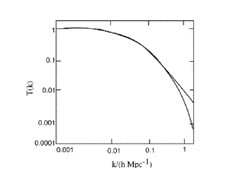
Figure 12: Transfer function for gravitinos and CDM showing their similarity, from [58]

Gravitinos, in my view, are not a particularly attractive form of dark matter, as to get the needed $\Omega_{3/2}$ one needs to have the gravitino mass ($m_{3/2}\sim\Lambda^{2}/M_{\rm P}$) finely tuned around a KeV. But this is not the worse trouble! Because of its extremely tiny interaction cross section [cf Eq. (67)] gravitino dark matter does not have any hope to be detected ever. In contrast, if the CDM is due to a neutralino LSP, in principle, it may be detectable by experimental means.

Calculation of the rates expected in low background experiments (for instance, those using a ${}^{73}{\rm Ge}$ detector of sufficient mass), depend both on the density of LSPs in our galaxy and on the neutralino-nucleon scattering cross section. This latter cross section depends again on the various parameters in the supersymmetric model. Except for very light nuclei, it turns out that scalar exchange dominates, since it leads to coherent scattering of the neutralinos on the target nuclei, so that $\sigma_{\chi A}\sim A^{2}$. Fig. 13 shows that the expected rates of neutralino CDM for a ${}^{73}{\rm Ge}$ detector are of the order of $10^{-2}-10^{-3}$ events/Kg-day. Given that present-day detectors (e.g. CDMS [59]) are operating with at best one Kg of Ge, one is still looking for a factor of $10^{2}-10^{3}$ improvement to have some hope of detecting a potential signal for neutralino cold dark matter. This is a daunting, but perhaps not impossible, task. As I said earlier, the experimental observation of a neutralino LSP in a particle physics experiment would give enormous impetus to the lofty goal of direct dark matter detection!

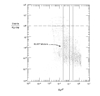
Figure 13: Expected rates from neutralino dark matter, from [54]

7 Axions as CDM Candidates

Axions are pseudo Goldstone bosons associated with a spontaneously broken global chiral symmetry, $U(1)_{\rm PQ}$, introduced to “solve” the, so called, strong CP problem.[60] The Lagrangian of the electroweak and strong interactions, in general, possesses an effective interaction involving the gluon field strengths, $G_{a}^{\mu\nu}$ and their duals $\tilde{G}_{a}^{\mu\nu}$:

$${\cal{L}}_{\rm eff}=\bar{\theta}\frac{\alpha_{s}}{8\pi}G_{a}^{\mu\nu}\tilde{G}_{a\mu\nu}~{}.$$ (70)

This interaction breaks P, T, and CP and produces a very large neutron electric dipole moment unless the parameter $\bar{\theta}$ is very small. This is the strong CP problem—why is $\bar{\theta}$ so small? The imposition of an additional global chiral symmetry on the standard model suggested by Quinn and myself,[60] essentially serves to replace the $\bar{\theta}$ parameter by a dynamical field—the axion field.[62] Instead of the CP violating interaction (70) one now has instead, a CP-conserving effective interaction of the axion field $a(x)$ with the gluons:

$${\cal{L}}_{\rm PQ}=\frac{a}{f}\frac{\alpha_{s}}{8\pi}G_{a}^{\mu\nu}\tilde{G}_{a\mu\nu}~{},$$ (71)

where $f$ is a scale associated with the spontaneous breakdown of $U(1)_{\rm PQ}$.

The axion is the Nambu-Goldstone boson associated with the spontaneous breakdown of the $U(1)_{\rm PQ}$ symmetry. However, because this symmetry has a chiral anomaly—reflected in the appearance of the interaction (71)—the axion is not truly massless but acquires a small mass. This mass is slightly model-dependent, but is of order

$$m_{a}\sim\frac{m_{\pi}f_{\pi}}{f}\sim\left(\frac{6\times 10^{6}}{f[{\rm GeV}]}\right)~{}{\rm eV}~{}.$$ (72)

One sees that, for large $f$, axions are very light. Since all couplings of the axion scales as $1/f$, these particles, if they exist, are also very weakly coupled. Although axions are not stable since they can decay into two photons, the lifetime for the process $a\to 2\gamma$ scales as $\tau\sim f^{5}$[61] and becomes enormous for large $f$.

Quinn and I[60] made the natural assumption that the scale of $U(1)_{\rm PQ}$ breaking coincided with the electroweak scale, $f\sim v$. Unfortunately, these weak-scale axions have been ruled out experimentally.[61] If $f$ is not of $O(v)$, it turns out that astrophysics constrains $f\gg v$. This is easy to understand. Axions provide an extremely efficient way to cool down stars, completely affecting their evolution. Only if $f\geq 5\times 10^{9}~{}{\rm GeV}$, are axion couplings sufficiently weak so as not to run into trouble with a variety of astrophysical observations—ranging from the evolution of red giants, to properties of the observed neutrino pulses from SN 1987a.[63] For $f\geq 5\times 10^{9}~{}{\rm GeV}$, the axions are so light, so weakly coupled, and so long-lived to be effectively “invisible”.[64] However, these invisible axions have potential cosmological consequence, and they prove to be interesting cold dark matter candidates! Let me review the arguments for this.[65]

Axions are typical non-thermal relics, since their properties change as the Universe evolves. At the $U(1)_{\rm PQ}$ phase transition, which occurs when the Universe’s temperature $T\sim f$, axions are produced as real Nambu-Goldstone bosons $(m_{a}=0)$. At such high temperatures the axion potential due to QCD is ineffective and the $\bar{\theta}$ interaction of Eq. (70) is not cancelled out. As the Universe cools towards temperatures of order of the QCD-scale $\Lambda_{\rm QCD},~{}T\sim\Lambda_{\rm QCD}$, two things happen: the axion potential turns on, serving to cancel $\bar{\theta}$, and the axion acquires its mass, which is of $O(\Lambda^{2}_{\rm QCD}/f)$. This relaxation of the axion field to its present configuration, however, happens in an oscillatory way. The energy density associated with these oscillations, as we shall see, acts as cold dark matter.[65]

The $\bar{\theta}$ parameter in Eq. (70) can be thought of as an effective VEV for the axion field: $\langle a\rangle=\bar{\theta}f$, with the correct vacuum state driving $\langle a\rangle\to 0$. In the early Universe at $T\sim f$, in this language, the axion field has an effective vacuum expectation $\langle a\rangle=\bar{\theta}f$. As the temperature lowers towards $T\sim\Lambda_{\rm QCD}$, the QCD potential for the axion turns on and $\langle a\rangle$ is driven to zero. One can study the time evolution of $\langle a\rangle$ by studying the equation of motion for the axion field in the expanding Universe:[65]

$$\frac{d^{2}\langle a\rangle}{dt^{2}}+3\frac{\dot{R}(t)}{R(t)}\frac{d\langle a\rangle}{dt}+m_{a}^{2}(t)\langle a\rangle=0~{}.$$ (73)

It is clear from the above that the effect of the expansion of the Universe is to provide a drag term for $\langle a\rangle$. At early times, or high temperatures, the axion mass vanishes and $\langle a\rangle$ is fixed to its initial value $\langle a\rangle=f\bar{\theta}$. When the axion mass $m_{a}(t)$ begins to turn on, as the Universe’s temperature cools towards $T\sim\Lambda_{\rm QCD}$, $\langle a\rangle$ undergoes damped oscillations about $\langle a\rangle=0$.

I shall not try to sketch here the computation of the effective energy density associated with these oscillations of $\langle a\rangle$, but refer to Ref.[61] for an elementary discussion. I quote, however, the result of a recent detailed calculation[66] which gives the contribution to $\Omega_{0}$ of these oscillations. One finds:

$$\Omega_{a}h^{2}=C\left[\frac{f}{10^{12}~{}{\rm GeV}}\right]^{n}\bar{\theta}^{2}~{}.$$ (74)

Here $C$ is a constant of $O(1)$ which depends on the details of the QCD phase transition, while the exponent $n$ is near unity, $n=1.18$. One sees that if the initial value for $\langle a\rangle/f=\bar{\theta}$ is of $O(1)$—as one may expect naively—then these oscillations of the axion VEV can close the Universe if $f\sim 10^{12}~{}{\rm GeV}$. Because what is oscillating is $\langle a\rangle$, these oscillations correspond physically to coherent, zero momentum, oscillations of the axion field. Since $\vec{p}_{a}=0$, axion oscillations are prototypical cold dark matter.

From the above, it appears that coherent axion oscillations can give rise to $\Omega=1$ provided $f\simeq 10^{12}~{}{\rm GeV}$ or $m_{a}\simeq 6\times 10^{-6}~{}{\rm eV}$. This is predicated on having an initial misallignment angle $\bar{\theta}\sim O(1)$. However, Linde[67] has argued that in inflationary cosmology, with the reheating temperature $T_{\rm reheating}<f$ so that there is not a post-inflationary $U(1)_{\rm PQ}$ phase transition, there is no reason why the misallignment angle cannot be very small: $\bar{\theta}^{2}\ll 1$. In this case one could have $\Omega_{a}\sim O(1)$ for smaller axion masses (or $f\gg 10^{12}~{}{\rm GeV}$):

$$\Omega_{a}\sim O(1)~{}~{}\hbox{if}~{}~{}m_{a}\simeq 6\times 10^{-6}\bar{\theta}^{2}~{}{\rm eV}~{}.$$ (75)

There are other arguments, however, which suggest that axion masses much heavier than $m_{a}\simeq 6\times 10^{-6}~{}{\rm eV}$ can close the Universe. These arguments apply in inflationary scenarios where the reheating temperature $T_{\rm reheating}>f$. In this case, one must worry about axionic strings formed at the $U(1)_{\rm PQ}$ phase transition. The decay of these strings into axions also contributes to the Universe’s energy density and this contribution can dominate that due to coherent axion oscillations.[68] Unfortunately, there is considerable controversy on this point, with some authors—notably P. Sikivie and collaborators[69]—obtaining $\Omega_{\rm string~{}decay}\sim\Omega_{\rm oscillation}$, with others[70] deducing $\Omega_{\rm string~{}decay}\gg\Omega_{\rm oscillation}$. If one were to believe this latter estimate, then one obtains $\Omega_{a}\sim O(1)$ for axion masses as heavy as $m_{a}\sim 10^{-4}~{}{\rm eV}$. These masses are perilously close to the mass range excluded by astrophysics, [63] $m_{a}\geq 10^{-3}~{}{\rm eV}$, corresponding to $f<5\times 10^{9}~{}{\rm GeV}$.

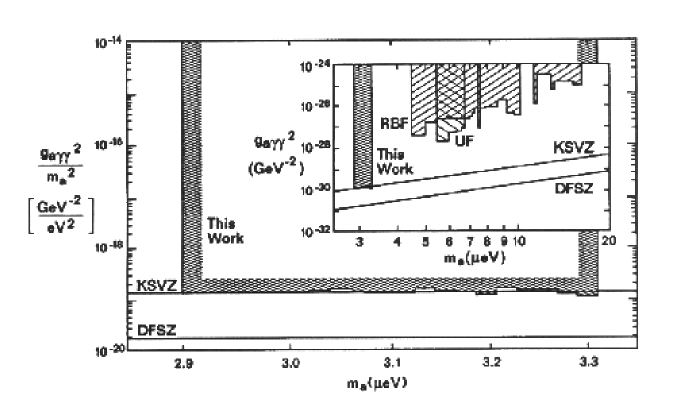
Figure 14: Results of invisible axion searches

These controversies may be resolved experimentally if axions are the dark matter in the Universe (and hence are also the dominant form of the dark matter in our galaxy!). The basic idea for these experiments is due to Sikivie[71] and uses the fact that axions couple to the electromagnetic field in a way analogous to how they couple to gluons [cf. Eq. (71)]:

$${\cal{L}}_{a\gamma\gamma}=g_{a\gamma\gamma}a\vec{E}\cdot\vec{B}$$ (76)

with $g_{a\gamma\gamma}\sim 1/f$. Because of Eq. (76) axions in our galactic halo in the presence of a strong magnetic field can be resonantly converted into photons in an appropriate cavity. Experiments are presently underway at both the Lawrence Livermore Laboratory[72] and at Kyoto University[73] which are sensitive to “standard” invisible axions if they are the dominant form of dark matter. Fig. 14 shows recent results from the Livermore experiment [72] in the $g^{2}_{a\gamma\gamma}-m_{a}$ plane (along with some regions already excluded by some initial pioneering experiments)[74] and the theoretical expectations of invisible axion models. The hope is that when both the Livermore and Kyoto experiments are completed, in 3-5 years, one will know whether axions are, or are not, an important component of the dark matter in the Universe

8 Perspectives on Dark Matter

It is useful at this stage to try to bring some perspective on the issue of dark matter from a particle physics point of view. As we saw, particle physics provides an interesting array of dark matter candidates. Among these, it appears that perhaps the neutralino LSP is the particle physics relic which is the most plausible dark matter candidate. In the simplest supersymmetric extension of the standard model, the MSSM, there is a rather large range in parameter space which gives rise to a neutralino LSP that has $\Omega_{\chi}h^{2}\sim O(1)$. In contrast, both for axions, gravitinos and neutrinos, the critical density in the Universe obtains only for some specific values of the parameters characterising these excitations (e.g. for axions one needs the scale of $U(1)_{\rm PQ}$ breaking, $f$, to be of $O(10^{12}~{}{\rm GeV})$).

Although, on the face of it, the above argument seems very reasonable, I am not sure it is totally compelling. For instance, in a similar vein one could argue also that having $\Omega_{B}=0.05$ is unnatural, since it requires a peculiar tuning of the nucleon mass! I believe a more sensible point of view to take is the following. Of all the cosmological scenarios, the inflationary scenario for the Universe appears to make the most sense. If this scenario is correct, then $\Omega=1$ is a boundary condition one should seriously impose as a constraint on the sum of all the particle species which are important in the Universe today. That is, we should demand that

$$1=\Omega=\sum_{1}\Omega_{i}~{}.$$ (77)

The particular weight of each of the components $\Omega_{i}$ in Eq. (77) is a reflection of intrinsic particle physics properties. The only cosmological constraint is that the sum of the $\Omega_{i}$ must add up to unity. So, if particle physics arguments lead to $f\simeq 10^{12}~{}{\rm GeV}$, or $m_{\nu_{\tau}}\simeq 5~{}{\rm eV}$, then that particular component will be important in the sum appearing in Eq. (77). From this point of view, “what you see is what you get”! If the parameters in the neutrino sector lead to some neutrino masses being in the eV range, then $\Omega_{\nu}$ is an important component of $\Omega$. If that is not the case, then $\Omega_{\nu}$ is not important. So, from this view point, there is no difference in pedigree between dark matter which is a significant component for a range of particle physics parameters (like the LSP), or relics which are important only for the specific value of some particle physics parameters (like a KeV gravitino).

Adopting this point of view then, it is perfectly sensible to have various particle physics excitations (say: baryons, neutralinos and neutrinos) play an important role in the Universe now. This is a welcome result, which is reinforced by the power spectrum of density fluctuations in the Universe. This spectrum also suggests that there is more than one component which contributes to the energy density of the Universe. Indeed, present data on this spectrum seems to be best fit by having a variety of matter components contributing. For instance, recent work by Primack and collaborators[75] suggests that the power spectrum of density fluctuations is optimally fit by having

$$\Omega_{\rm B}=0.05;~{}~{}~{}\Omega_{\rm CDM}=0.75;~{}~{}~{}\Omega_{\rm HDM}=0.20~{}.$$ (78)

These results are particularly interesting since the existence, or not, of HDM provides a critical constraint (arising from cosmology) on the particle physics which determines the neutrino mass matrix. If it were really possible to establish the need for neutrino hot dark matter, for example through the influence it has on the angular spectrum of the CMBR,[43] then this, along with the constraints imposed by neutrino oscillation experiments would do much to fix the shape of the neutrino mass spectrum. As we discussed earlier, if one can establish both the need for neutrino hot dark matter (which necessitates probably that $\sum_{i}m_{\nu_{i}}\simeq(5-6~{}{\rm eV})$) and of neutrino oscillations with small mass squared differences, then one is forced into a world of nearly degenerate neutrino masses, with $m_{\nu_{i}}\simeq 1-2~{}{\rm eV}$. Such a result would provide a compelling argument for renewing the direct searches in tritium beta decay for electron neutrino masses in the eV range.

9 The Sakharov Conditions for Baryogenesis

In a classic paper, in 1967, Andrei Sakharov[1] discussed the conditions necessary to obtain dynamically an asymmetry between matter and antimatter in the Universe. Sakharov’s conditions for obtaining this asymmetry are three-fold:[1]

(i) The underlying physical theory must possess processes that violate baryon number (B is not conserved).

(ii) The interactions which lead to B-violation, in addition must violate C and CP.

(iii) To establish this asymmetry dynamically, furthermore, the B-violating processes must be out of equilibrium in the Universe.

Let me comment briefly on each of these points. First, it is pretty clear that if B is conserved then the total number of baryons minus anti-baryons is a constant in time. In this case, then the difference $n_{\rm B}-n_{\rm\bar{B}}$ is a constant that is set by some initial boundary conditions. Thus $\eta$ is not generated dynamically, but is just a reflection of these initial boundary conditions and one is left to wonder why one has a value $\eta\sim 10^{-10}$.

Similarly, it is also quite understandable why the second Sakharov condition is needed. If C and CP are good symmetries, one can transform $n_{\rm B}$ into $n_{\rm\bar{B}}$ by one of these symmetry transformations. Hence, even if B were to be violated, but if C or CP were to be good symmetries, then one could never obtain a non-vanishing value for $\eta$.

The third Sakharov condition is slightly more subtle, but is also readily understandable physically. Roughly speaking, B-violating decays serve to create a matter-antimatter asymmetry. However, this asymmetry is destroyed by inverse decays. In thermal equilibrium, the rates for B-violating decays and their inverses are the same, hence $n_{\rm B}-n_{\rm\bar{B}}=0$.

It is useful to demonstrate this last fact explicitly. The rate of change of $\Delta n_{\rm B}=n_{\rm B}-n_{\rm\bar{B}}$ as a result of B-violating processes, if these processes are in equilibrium, is given by the thermodynamic equation

$$\frac{d\Delta n_{\rm B}}{dt}=\gamma_{\not{\mbox{B}}}e^{-\mu/T}-\gamma_{\not{\mbox{B}}}e^{\mu/T}~{}.$$ (79)

Here $\gamma_{\not{\mbox{B}}}$ is the rate of B-violation per unit volume and $\mu$ is the chemical potential. At high temperatures, one can expand the exponential factors and the above expression reduces to

$$\frac{d\Delta n_{\rm B}}{dt}\simeq-\frac{2\mu}{T}\gamma_{\not{\mbox{B}}}~{}.$$ (80)

However, in this temperature regime, one has simply that

$$\Delta n_{\rm B}=\frac{4}{\pi^{2}}\mu T^{2}~{}.$$ (81)

Hence

$$\frac{d\Delta n_{\rm B}}{dt}\simeq-\frac{\pi^{2}}{2}\left(\frac{\gamma_{\not{\mbox{B}}}}{T^{3}}\right)\Delta n_{\rm B}=-\frac{\pi^{2}}{2}\Gamma_{\not{\mbox{B}}}\Delta n_{\rm B}~{},$$ (82)

where $\Gamma_{\not{\mbox{B}}}$ is just the rate for B-violation, since $V=T^{-3}$. Thus, it follows from (82) that

$$\Delta n_{\rm B}=(\Delta n_{\rm B})_{0}\exp\left[-\frac{\pi^{2}}{2}\Gamma_{\not{\mbox{B}}}t\right]~{}.$$ (83)

Eq. (83) tells one that, if B-violating processes are ever in equilibrium, then these processes serve to destroy any pre-existing asymmetry $(\Delta n_{\rm B})_{0}$. This is a very nice result[76] since it tells us that the value of $\eta$ one computes dynamically, as a result of B-violating processes going out of equilibrium, is independent of any initial asymmetry $(\Delta n_{\rm B})_{0}$. Hence, the observed value of $\eta$ in the Universe now depends only on the B-violating (and C- and CP-violating) dynamics—due to particle physics—and on the cosmology which drives these processes out of equilibrium in the early Universe.

I examine next cosmological circumstances (along with the relevant particle physics) which can lead to baryogenesis.

10 Baryogenesis at the GUT Scale: Issues and Challenges

Grand Unified Theories (GUTs) were the first theories which explicitly realized Sakharov’s conditions for baryogenesis.[77] These theories naturally contain B-violating processes which also violate C and CP. An example is provided by $SU(5)$,[78] in which the fermions of each generation are members of a $\bar{5}\sim(d^{c}_{\rm L};e_{\rm L}\nu_{\rm L})$ and a $10\sim(u_{\rm L}d_{\rm L};u^{c}_{\rm L};d^{c}_{\rm L})$ representation and the ordinary Higgs doublet $(\phi^{+}\phi^{0})$ is augmented by a Higgs triplet $\chi$ into a field $5_{\rm H}\sim(\chi;\phi^{+}\phi^{0})$—with $\chi$ transforming under $SU(3)\times SU(2)\times U(1)$ as $\chi\sim(3,1)_{-1/3}$. In $SU(5)$, the Higgs quintet $5_{\rm H}$ can couple to the fermions in two separate ways $[5_{\rm H}~{}5~{}\overline{10}~{}\hbox{and}~{}5_{\rm H}~{}10~{}10]$, with the corresponding complex Yukawa couplings being sources for C and CP violation. These couplings allow the triplet Higgs field $\chi$ to decay to both the $d\nu$ (B = 1/3) and $\bar{u}\bar{d}$ (B = -2/3) final states. Hence, in $SU(5)$ baryon number is clearly not conserved.

Because one knows experimentally that baryon number is conserved to high accuracy, one knows that a theory like $SU(5)$, where the $SU(3)$, $SU(2)$ and $U(1)$ forces are unified, must break down to $SU(3)\times SU(2)\times U(1)$ at a very high scale: $M_{X}\sim 10^{15}-10^{16}~{}{\rm GeV}$.[79] This unification scale $M_{X}$ is quite near the Planck scale $M_{\rm P}\sim 10^{19}~{}{\rm GeV}$. We know that at temperatures near the Planck scale, $T\sim M_{\rm P}$, the Universe is expanding very rapidly. Thus it is not surprising that the C, CP and B-violating decays of GUTs have rates which are slow with respect to the expansion rate of the Universe at $T\sim M_{X}$. That is

$$\frac{\dot{R}}{R}\sim\frac{T^{2}}{M_{\rm P}}>\Gamma_{\rm B-viol.}~{}~{}~{}~{}~{}~{}(T\sim M_{X})~{}.$$ (84)

Hence, the processes alluded above in GUTs also fulfill Sakharov’s third condition—that the relevant B-, C-, and CP-violating interactions be out of equilibrium in the early period of expansion of the Universe after the Big Bang.

These qualitative features, however, in practice do not lead to successful simple scenarios for baryogenesis at the GUT scale. Although it is possible to obtain $\eta\sim 10^{-10}$ in some GUT models, these models have a number of generic difficulties which are worth discussing here. Again, it is useful to consider the $SU(5)$ example alluded above to help focus on the source of these difficulties.

In $SU(5)$, the ratio $\eta$ is generated through the out of equilibrium decay of the Higgs triplet $\chi$ at temperatures $T\sim M_{X}$. One has

$$\eta=\frac{n_{\rm B}-n_{\bar{\rm B}}}{n_{\gamma}}\simeq A\Delta{\rm B}_{\chi}~{}.$$ (85)

Here $A$ is a kinematical/dynamical factor related to the way the $\chi$ decays go out of equilibrium, while $\Delta B_{\chi}$ is the baryon asymmetry proper:

$$\Delta B_{\chi}=\sum_{f}\frac{B_{f}\{\Gamma(\chi\to f)-\Gamma(\bar{\chi}\to\bar{f})\}}{\Gamma_{\chi}^{\rm total}}~{},$$ (86)

reflecting the differences in the weighted ratio of $\chi$ and $\bar{\chi}$ decays into particular final states $f$ with different baryon number $B_{f}$. It should be clear from the form of Eq. (86) that $\Delta B_{\chi}$ vanishes if C or CP is conserved, since then $\Gamma(\chi\to f)=\Gamma(\bar{\chi}\to\bar{f})$.

It is easy to see that, for the example in question, one has simply

$$\Delta B_{\chi}=r-\bar{r}$$ (87)

where

$$r=\frac{\Gamma(\chi\to d\nu)}{\Gamma_{\chi}^{\rm total}}~{};~{}~{}~{}~{}~{}~{}\bar{r}=\frac{\Gamma(\bar{\chi}\to\bar{d}\bar{\nu})}{\Gamma_{\chi}^{\rm total}}~{}.$$ (88)

Eq. (87) has three characteristics:

(i) It vanishes if there is no C or CP violation. This is obvious, since then $\bar{r}=r$.

(ii) $\Delta B_{\chi}$ vanishes also if one includes only lowest order processes. Again this is easy to see since, at tree level, $r=\bar{r}$.

(iii) Finally, and less obviously, $\Delta B_{\chi}$ also vanishes if the underlying $\chi$-decays do not have an s-channel discontinuity.

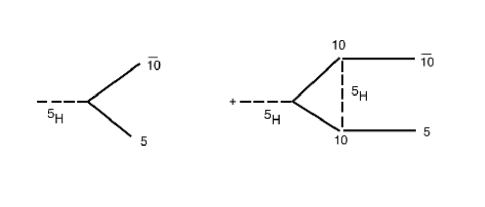
Figure 15: Graphs contributing to $r$ at one-loop order

One can see these three conditions at work by examining schematically the contribution to $r$ in the $SU(5)$ model we discussed earlier. At one-loop order, these contributions are given by the graphs shown in Fig. 15. Let us denote by $\gamma_{0}$ the rate associated with the tree graph decay in Fig. 15 and by $\gamma_{1}I(M_{\chi}^{2}-i\epsilon)$ the contribution of the one-loop graph. In general both $\gamma_{0}$ and $\gamma_{1}$ are intrinsically complex as a result of the complex $\chi$ couplings, while the dynamical quantity $I(M_{\chi}^{2}-i\epsilon)$ has an imaginary part as a result of the associated loop integration. A simple calculation, using Fig. 15, gives for the rate difference $r-\bar{r}$ the expression:

$$(r-\bar{r}) \sim |\gamma_{0}+\gamma_{1}I(M^{2}_{\chi}-i\epsilon)|^{2}-|\gamma_{0}^{*}+\gamma_{1}^{*}I(M_{\chi}^{2}-i\epsilon)|^{2}$$ (89)

$$\sim {\rm Im}~{}\gamma_{0}\gamma_{1}^{*}~{}~{}{\rm Im}~{}(I(M_{\chi}^{2}-i\epsilon))~{}.$$

One sees that this rate difference vanishes unless there is both an intrinsic CP violating phase difference in the couplings involved [Im $\gamma_{0}\gamma_{1}^{*}$] as well as some imaginary part [Im $(I(M_{\chi}^{2}-i\epsilon))$ ] arising from the (one-loop) scattering dynamics. In view of Eq. (89), one sees that the ratio $\eta=\Delta n_{\rm B}/n_{\gamma}$ is proportional to

$$\eta=A\Delta B_{\chi}=A(r-\bar{r})\sim A~{}{\rm Im}~{}\gamma_{0}\gamma_{1}^{*}~{}{\rm Im}~{}I~{}.$$ (90)

The RHS of Eq. (90) embodies the essence of GUT baryogenesis. The ratio $\eta$ depends on the out of equilibrium dynamics [through $A$] and it vanishes unless there is both an intrinsic CP and C violating phase [Im $\gamma_{0}\gamma_{1}^{*}$] and the GUT dynamics is rich enough to generate an s-channel discontinuity[Im $I(M^{2}_{\chi}-i\epsilon)$]. The knowledge of each of these individual pieces is clearly model-dependent and quite rudimentary, since we have no direct evidence for the existence of any GUTs ! Thus, at this stage, it is really not possible to deduce a firm prediction for $\eta$. Even so, in general, one finds $\eta$ to be too small unless one further complicates the GUT dynamics.

Let me illustrate the above point in the, by now familiar, $SU(5)$ context. Without loss of generality one can make the $5_{\rm H}~{}5~{}\overline{10}$ Higgs coupling matrix $f$ real. Then it is easy to show that (for 3 families) the $5_{\rm H}~{}10~{}10$ coupling matrix $h$ has 3 phases.[80] So GUTs, because they involve further Higgs couplings, have more phases than the 3-family CKM phase connected with the couplings of the Higgs doublet $\Phi$ to quarks. Even so, in this model, one cannot generate an intrinsic CP violating phase at one loop order. The tree and one-loop level contributions in Fig. 15, corresponding to the process $5_{\rm H}\to 10~{}\bar{5}$, give

$$\gamma_{0}\sim f~{};~{}~{}\gamma_{1}\sim fhh^{{\dagger}}~{}.$$ (91)

Hence

$${\rm Im}~{}\gamma_{0}\gamma_{1}^{*}\sim{\rm Im}~{}{\rm Tr}~{}fhh^{{\dagger}}f^{{\dagger}}=0~{}.$$ (92)

One can check that other possible contributions to the decay $5_{\rm H}\to 10~{}\bar{5}$, involving gauge exchange in the $t$-channel rather than Higgs exchange, are similarly relatively real. As shown in Fig. 16, one can eventually[81] obtain a non-vanishing $\eta$ for this model at higher order, from the interference of a tree-level process with a 3-loop process. The resulting $\Delta B_{\chi}$, however,

$$\Delta B_{\chi}\sim{\rm Im}~{}{\rm Tr}[h^{{\dagger}}ff^{{\dagger}}hff^{{\dagger}}h^{{\dagger}}h]$$ (93)

has such a large number of Yukawa couplings that $\eta$ is at best of $O(10^{-15})$.[81]

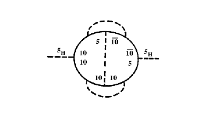
Figure 16: Interference graph giving $r\neq 0$ in $SU(5)$

This difficulty can be remedied by using more elaborate GUTs (or including more low-energy states). However, there are two further generic problems connected with these types of models which serve to dampen the enthusiasm for attributing baryogenesis in the Universe to some GUT processes. The first of these additional problems is related to monopoles. In general GUTs lead to an overproduction of monopoles in the early Universe, badly violating one of the main features we know about the Universe now–namely that the present Universe’s energy density is near the critical density $\rho\sim\rho_{c}$.[2]

’t Hooft and Polyakov[83] showed that monopoles always form when a symmetry group breaks down to a subgroup containing a $U(1)$ factor–like the standard model group. Hence, if GUTs exist, one expects that in the very early Universe at $T\sim M_{X}$, during the GUT phase transition, magnetic monopoles are formed. Generically, these GUT monopoles are superheavy, having a mass of order $M_{\rm M}\sim\frac{M_{X}}{\alpha_{\rm G}}\sim 10^{17}~{}{\rm GeV}$. During the GUT phase transition, domains of the broken phase of the GUT group form which are of typical size $\xi\sim\frac{1}{T_{c}}\sim\frac{1}{M_{X}}$. The superheavy GUT monopoles physically correspond to topological knots between these domains and hence have a density $n_{\rm M}\sim\xi^{-3}$. This density is comparable to the photon density at this stage of the Universe

$$n_{\rm M}(T_{c})\sim\xi^{-3}\sim T_{c}^{3}\sim n_{\gamma}(T_{c})~{}.$$ (94)

However, such a large monopole density is extremely problematic, because of the large mass of the GUT monopoles .[2] Indeed, from (94) one deduces that

$$\Omega_{\rm M}\big{|}_{\rm now}\sim M_{\rm M}n_{\gamma}\big{|}_{\rm now}\sim 10^{21}$$ (95)

completely in contradiction with what we know!

Inflation provides a resolution of the monopole problem by inflating exponentially the size of the domains—essentially reducing the monopole density to one per observable Universe. However, to re-establish $\eta$ in such a scenario, one has to reheat the Universe after the inflationary period to temperatures $T_{\rm reheat}\sim 10^{14}-10^{15}~{}{\rm GeV}$, which is difficult to achieve.[84] Thus, the monopole problem, even if it is resolved by inflation, argues against GUT baryogenesis.

There is another argument which also provides ammunition against the idea that the baryon asymmetry in the Universe was produced at the GUT scale. As we will discuss shortly in more detail, it turns out that quantum effects in the electroweak interactions can lead to the violation of total fermion number (B+L—violation).[4] In the middle 1980’s Kuzmin, Rubakov and Shaposhnikov (KRS)[5] argued that these (B+L)-violating processes, which are extremely weak at $T=0$, could become strong enough at temperatures near the electroweak phase transition, $T\sim M_{W}$, to go back into equilibrium in the Universe. The return of (B+L)-violating processes into equilibrium in the Universe at $T\ll M_{X}$ serves to erase any (B+L)-asymmetry produced in the Universe at temperatures of the order of the GUT scale, $T\sim M_{X}$. Hence, only a (B-L) asymmetry produced by GUTs survives to low temperatures.

This consideration kills, for example, the baryon number asymmetry one imagined was produced in the $SU(5)$ example discussed earlier. It is easy to check that for $\chi$-decays

$$\Delta B_{\chi}=\Delta L_{\chi}=r-\bar{r}~{},$$ (96)

so that

$$\Delta n_{\rm B-L}=\Delta n_{\rm B}-\Delta n_{\rm L}=0~{}.$$ (97)

Thus, as a result of the KRS mechanism, in this case no baryon asymmetry survives at low temperatures, even if such an asymmetry were to be generated at the GUT scale by the out of equilibrium decays of the Higgs triplet $\chi$. Of course, one can invent more elaborate GUTs scenarios in which at the GUT scale one produces both a (B+L)- and a (B-L)-asymmetry, thereby bypassing this conundrum.[85]

11 The KRS Mechanism and Baryogenesis at the Electroweak Scale

In this section I want to discuss further the KRS mechanism[5] because, besides erasing any previous (B+L)–asymmetry, it is possible that through this mechanism one can actually produce the observed baryon asymmetry in the Universe during the electroweak phase transition. This is an exciting possibility, and one that has received considerable attention in recent years.[86] In the Standard Model, both baryon number, B, and lepton number, L, are classical symmetries. That is, they are symmetries of the Standard Model Lagrangian:

$${\cal{L}}_{\rm SM}\begin{array}[]{c}\\[-7.22743pt] \longrightarrow\\[-7.22743pt] \mbox{\tiny L,B}\end{array}{\cal{L}}_{\rm SM}~{}.$$ (98)

However, because of the chiral nature of the electroweak interactions, at the quantum level both the baryon number current, $J_{\rm B}^{\mu}$, and the lepton number current, $J_{\rm L}^{\mu}$, are not conserved. Hence neither B, nor L, remains a good symmetry at the quantum level, although their difference, B-L, is still a conserved quantum number.

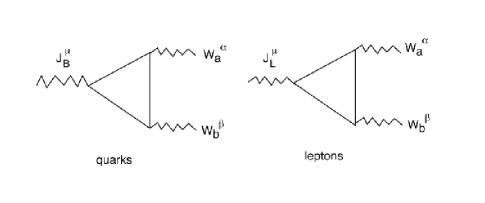
Figure 17: Triangle graphs contributing to the B and L anomalies

The violation of B and L in the standard model comes about as a result of the existence of chiral anomalies[87] in their respective currents. For our purposes, it suffices to focus only on the $SU(2)$ gauge field contribution to this anomaly. The triangle graphs contributing to the anomalous divergence of $J_{\rm B}^{\mu}$ and $J_{\rm L}^{\mu}$ are shown in Fig. 17 and produce an equal divergence for both currents[87]

$$\partial_{\mu}J_{\rm B}^{\mu}=\partial_{\mu}J_{\rm L}^{\mu}=-N_{g}\frac{\alpha_{2}}{8\pi}W_{a}^{\mu\nu}\tilde{W}_{a\mu\nu}~{},$$ (99)

where $N_{g}$ is the number of generations and $\alpha_{2}=g_{2}^{2}/4\pi$. Clearly it follows then that

$$\partial_{\mu}J_{\rm B-L}^{\mu} = 0$$

$$\partial_{\mu}J_{\rm B+L}^{\mu} = -N_{g}\frac{\alpha_{2}}{4\pi}W_{a}^{\mu\nu}\tilde{W}_{a\mu\nu}~{}.$$ (100)

These equations, per se, do not automatically lead to a violation of (B+L)-number. To get a change in B+L [$\Delta({\rm B+L})\not=0$] requires having processes involving non Abelian gauge field configurations which have a non-trivial index $\nu$:

$$\nu=\frac{\alpha_{2}}{8\pi}\int d^{4}xW_{a}^{\mu\nu}\tilde{W}_{a\mu\nu}~{},$$ (101)

since, in view of (100),

$$\Delta({\rm B+L})=2N_{g}~{}\nu~{}.$$ (102)

’t Hooft[4] was the first to estimate the size of the amplitudes which contain gauge field configurations having such a non-trivial index $\nu$. These amplitudes arise in processes where the pure gauge field configurations at $t=+\infty$ and $t=-\infty$ differ by a so-called, “large” gauge transformation[88]. In the $A^{o}=0$ gauge, pure gauge fields can be classified by how their associated gauge transformations go to unity at spatial infinity

$$\Omega_{n}{(\vec{r})}\begin{array}[]{c}\\[-7.22743pt] \longrightarrow\\[-7.22743pt] \mbox{\tiny${\vec{r}}\to\infty$}\end{array}e^{2\pi in}.$$

One can show that the index $\nu$ is related to the difference in the indices $n_{\pm}$ characterizing the gauge vacuum configurations at $t=\pm\infty$ [$\nu=n_{+}-n_{-}$].[88] ’t Hooft’s estimate[4] of the size of the amplitudes leading to (B+L) violation essentially involved the WKB probability for tunneling from a vacuum characterized by index $n$ to one where the index was $n+\nu$. His result[4]

$$A_{\rm(B+L)-violating}\sim{\rm exp}\left[-\frac{2\pi}{\alpha_{2}}\nu\right]$$ (103)

has a typical WKB form, involving the inverse of the gauge coupling constant squared in the exponent. However, since the weak coupling constant squared $\alpha_{2}$ is very small $(\alpha_{2}\sim 1/30)$, the result (104) is extraordinarily tiny: $A_{\rm(B+L)-violating}\sim 10^{-80\nu}$ !

’t Hooft’s result (104) is valid at $T=0$. What Kuzmin, Rubakov and Shaposhnikov[5] realized was that the situation can be radically different in the early Universe, when the (B+L)-violating processes happen in a non-zero thermal background. When $T\not=0$, the gauge vacuum change needed for $\Delta({\rm B+L})\not=0$ transitions to happen can occur not only by tunneling, but also via a thermal fluctuation. In this latter case, the transition probability is not given by the square of the WKB amplitude (104), but instead by a Boltzman factor:

$$P_{\rm(B+L)-violation}\sim{\rm exp}\left[-\frac{V_{o}(T)}{T}\right]~{}.$$ (104)

In the above, $V_{o}(T)$ is the (temperature dependent) height of the barrier which separates inequivalent gauge vacuum configurations.

It turns out that one can estimate $V_{o}$ also by semiclassical methods; in this case, by using a static solution of the electroweak theory with minimum energy and winding number $n=1/2$. This solution, first found by Klinkhamer and Manton[89], has been dubbed by them a sphaleron. Essentially, one takes $V_{o}(T)$ to be the energy associated with the sphaleron configuration in the presence of a thermal bath: $V_{o}(T)=E_{\rm sph}(T)$. This energy has the typical form expected of a classical extended object. It is proportional to the mass of the gauge field associated with the symmetry which suffers the breakdown and is inversely proportional to the gauge coupling constant [c.f. the formula characterizing the monopole mass]. For the sphaleron, one has

$$E_{\rm sph}=\frac{2M_{W}}{\alpha_{2}}f(M_{\rm H}/M_{W})~{},$$ (105)

where $f$ is a function of order unity.

Because the $W$ mass, $M_{W}(T)$, vanishes as the temperature $T$ approaches the temperature of the electroweak phase transition, $T\to T_{EW}$, the probability of (B+L)-violating processes occurring in the Universe becomes large as the Universe’s temperature approaches $T_{EW}$. This is basically the fundamental observation made by Kuzmin, Rubakov and Shaposhnikov.[5] That is, one expects that

$$P_{\rm(B+L)-violation}(T)\sim{\rm exp}\left[-\frac{E_{\rm sph}(T)}{T}\right]\begin{array}[]{c}\\[-7.22743pt] \longrightarrow\\[-7.22743pt] \mbox{\tiny$T\to T_{EW}$}\end{array}1~{}.$$ (106)

The original suggestion of KRS has been confirmed subsequently by much more detailed calculations.[90] Furthermore, one has found also a fast rate for (B+L)-violation, above the temperature of the electroweak phase transition.[91] These results are summarized below in a pair of formulas giving the transition probability per unit volume, per unit time, for temperatures below and above the temperature of the electroweak phase transition. One finds:

$$\gamma_{\rm(B+L)-violation} = C\left[\frac{M_{W}^{7}}{(\alpha_{2}T)^{3}}\right]{\rm exp}-\frac{E_{\rm sph}(T)}{T}~{}~{}~{}(T<T_{EW})$$

$$\gamma_{\rm(B+L)-violation} = C^{\prime}[\alpha_{2}T]^{4}~{}~{}~{}(T>T_{EW})~{},$$ (107)

where $C$ and $C^{\prime}$ are constants of order one. These results imply that the rate of (B+L)-violating processes, originating in the standard model, is more rapid than the Universe’s expansion rate $H\sim T^{2}/M_{\rm P}$ for rather a large temperature interval:[92]

$$\Gamma_{\rm(B+L)-violation}=\frac{\gamma_{\rm(B+L)-violation}}{T^{3}}>H~{}~{}{\rm for}~{}~{}T_{EW}\sim 10^{2}~{}{\rm GeV}\leq T\leq 10^{12}~{}{\rm GeV}~{}.$$ (108)

A consequence of the above is that any (B+L)-asymmetry established above $T_{\rm max}\sim\alpha_{2}^{4}M_{\rm P}\sim 10^{12}~{}{\rm GeV}$ (by, for example, some GUT processes) will get washed out.

Given these results, two possibilities emerge for trying to explain the observed value of $\eta\sim 10^{-10}$:

i) The baryon-antibaryon asymmetry underlying $\eta$ is the result of a (B-L), or perhaps simply an L, asymmetry generated at high temperatures. Since the baryon number can be written as

$$B=\frac{1}{2}(B+L)+\frac{1}{2}(B-L)~{},$$ (109)

and all the (B+L)-asymmetry is erased by the KRS mechanism, one needs to have some (B-L) asymmetry produced at high temperature to generate a non-vanishing value for $\eta$ now.

ii) The observed value of $\eta$ is the result of processes occurring at the electroweak phase transition. Baryogenesis is simply the reflection of the violation of (B+L) in the standard model–electroweak baryogenesis.

For the remainder of this section, I want to discuss this latter possibility. This is a very intriguing suggestion[93] and one which has generated an enormous amount of interest recently.[86] It is clear that to be able to generate $\eta$ at the electroweak phase transition, one needs this transition to be of first order, so as to get a deviation from thermal equilibrium. As one goes through the phase transition, the Higgs VEV, which vanished above $T_{EW}$, jumps to a non-zero value $\langle\phi(T^{*})\rangle$ for temperatures below that of the electroweak phase transition.

However, to try to obtain through this non-equilibrium processes $\eta\sim 10^{-10}$ needs much more than just having a first-order phase transition. There are actually two other main requirements. First, one must make sure that the asymmetry $\Delta n_{\rm B+L}$ created at the electroweak phase transition does not get erased by having the (B+L)-violating processes still be in equilibrium at $T^{*}$. This requires that

$$\Gamma_{\rm(B+L)-violation}(T^{*})=C\left[\frac{M_{W}^{7}}{\alpha_{2}^{3}T^{*6}}\right]{\rm exp}\left[-\frac{E_{\rm sph}(T^{*})}{T^{*}}\right]<H(T^{*})\sim\frac{T^{*2}}{M_{\rm P}}~{}.$$ (110)

Numerically, this condition is equivalent to the requirement[86]

$$\frac{E_{sph}(T^{*})}{T^{*}}\geq 45~{}~{}\hbox{or}~{}~{}\frac{\langle\phi(T^{*})\rangle}{T^{*}}\geq 1~{}.$$ (111)

That is, to avoid erasure of the produced $\Delta n_{\rm B+L}$ after the electroweak phase transition, this transition must be strongly first order, giving rise to a large jump for the Higgs VEV.

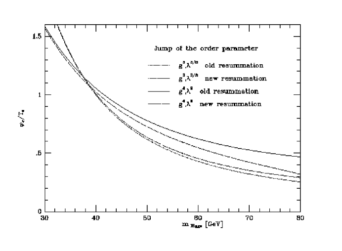
Figure 18: Jump in the order parameter in units of the critical temperature

One can compute the jump in $\langle\phi(T^{*})\rangle$ from the temperature-dependent effective potential for the electroweak theory. Although there are a number of uncertainties in this calculation,[94] it is now generally agreed[86] that in the Standard Model with only one Higgs doublet one cannot get a sufficiently strong first-order phase transition, unless the Higgs boson is light. The present LEP bounds on the Higgs boson mass, $M_{H}>77.5~{}{\rm GeV}$[95] are already sufficiently strong so as to rule out this simplest version of the Standard Model as the source of the Universe’s matter–anti-matter asymmetry. This is made clear by Fig. 18, taken from[94], which shows that for $M_{H}\sim 75~{}{\rm GeV}$ one expects $\langle\phi(T^{*})\rangle/T^{*}\simeq 0.5$, in contradiction with the requirement of Eq. (112). For such high values of the Higgs mass, standard model processes could create a baryon asymmetry $\Delta n_{\rm B+L}$ at the electroweak phase transition, but this asymmetry would then get destroyed again at $T^{*}$, since the rate of (B+L)-violation is still quite fast at this temperature compared to the Universe’s expansion rate.

The situation, in this respect, is considerably better in supersymmetric extensions of the Standard Model. Carena, Quiros and Wagner, [96] for example, recently showed that the inequality (112) can be satisfied in the MSSM, provided that one has a light stop, as well as small values for tan $\beta$ and a reasonably light Higgs. The values for $m_{\tilde{t}}$ and $m_{h}$ required by [96] to allow for baryogenesis at the weak scale are low enough that these particles should be observable in the near future already at LEP 200 and/or at the Tevatron, when the Main Injector is put into operation. So perhaps one may, in this way, soon get indirect evidence for electroweak baryogenesis.

The second important requirement for believing that baryogenesis occurred at the electroweak scale is to actually be able to carry out a detailed dynamical calculation for $\eta$, yielding $\eta\sim 10^{-10}$. Even if the electroweak phase transition is sufficiently strongly first order, so that the produced $\Delta n_{\rm B+L}$ is not erased, it is not obvious that one can produce a big enough $\Delta n_{\rm B+L}$ so as to give $\eta\sim 10^{-10}$.

In the case of electroweak baryogenesis, the matter-antimatter asymmetry is produced when bubbles of the true vacuum grow and fill up the Universe after the electroweak phase transition. As the Universe goes through the (assumed) first-order electroweak phase transition, CP-violating processes occurring in matter in the expanding bubble of true vacuum are crucial to establishing a matter-antimatter asymmetry. The rate of (B+L)-violation per unit volume, $\gamma_{\rm(B+L)-violation}$, is rapid in the symmetric vacuum surrounding the bubbles of true vacuum [$\gamma^{\rm outside}_{\rm(B+L)-violation}\sim(\alpha_{2}T)^{4}$]. However, by assumption, if Eq. (112) holds, within the bubbles of true vacuum this same rate is negligible [$\gamma^{\rm inside}_{\rm(B+L)-violation}\simeq 0$]. This rate difference is the key for establishing an asymmetry.

A full dynamical calculation of $\eta$ is very difficult. Nevertheless, one can sketch pictorially what is going on simply by thinking of the expanding true vacuum bubble as a wall sweeping through a plasma of quarks and antiquarks. Because of CP-violating processes in the wall, the scattering of quarks and antiquarks off the wall, as this wall sweeps through the plasma, is not the same. This difference in scattering will create an excess, say, of antiquarks over quarks in the symmetric vacuum, $-\Delta n_{q}$, and an opposite excess of quarks over antiquarks, $\Delta n_{q}$, in the true vacuum. The fast (B+L)-violating interactions in the symmetric vacuum, however, rapidly erase the antiquark excess, $-\Delta n_{q}$, leaving a quark excess, $\Delta n_{q}$, in the true vacuum bubble. This is the source of the baryon asymmetry.

There are many issues one has to resolve, or understand, to perform a reliable calculation of the above processes. For instance, what is the bubble wall thickness?; what is the bubble value velocity?; etc. Nevertheless, although an actual calculation is difficult, one can at least arrive at an order of magnitude estimate for $\eta$. Recall that the asymmetry is produced by the erasure of the antiquark excess in the symmetric vacuum. Hence

$$\eta\sim\frac{\gamma_{\rm B+L~{}violation}}{T^{3}}\Big{|}^{T^{*}}_{\rm sym~{}vacuum}\sim C^{\prime}\alpha_{2}^{4}T^{*}~{}.$$ (112)

If one assumes, quite naturally, that all time scales in the problem are set by $1/T^{*}$,[97] then the proportionality constant in Eq. (113)—besides the factor of $\alpha_{2}^{4}$—is set by the amount of CP-violation in the quark and antiquark scattering off the bubble wall. Calling this factor $\epsilon_{CP-violation}$, one arrives at the estimate

$$\eta\simeq[\alpha_{2}]^{4}\epsilon_{\rm CP-violation}\simeq 10^{-6}\epsilon_{\rm CP-violation}~{}.$$ (113)

This estimate is confirmed by more detailed calculations, like those done recently by Huet and Nelson.[97]

Taking Eq. (114) as a reasonable guesstimate for electroweak baryogenesis, one sees that this process is effective in creating a sufficiently large baryon-antibaryon asymmetry only if there is enough CP-violation! That is, one needs to generate in the bubble walls at least $\epsilon_{\rm CP-violation}\sim 10^{-4}$. It turns out, however, that the standard model of flavor violation—the CKM model[98]—fails miserably in this task. In this case, because of the GIM mechanism,[99] there is no CP-violation unless the quark masses are different. Whence, one expects in this case that $\epsilon_{\rm CP-violation}$ contains a number of GIM factors, which vanish if there is quark degeneracy. In particular, on general grounds, one expects

$$[\epsilon_{\rm CP-violation}]^{\rm CKM} \sim \frac{[\lambda^{6}\sin\delta]}{[T^{*}]^{12}}\cdot[(m_{t}^{2}-m_{u}^{2})(m_{t}^{2}-m_{c}^{2})(m_{c}^{2}-m_{u}^{2})$$ (114)

$$\cdot (m_{b}^{2}-m_{d}^{2})(m_{b}^{2}-m_{s}^{2})(m_{s}^{2}-m_{d}^{2})]~{}.$$

The first square bracket contains the usual family mixing suppression factor, [100] while the second factor involves a product of GIM factors. The result which follows from Eq. (115), $\epsilon^{\rm CKM}_{\rm CP-violation}\sim 10^{-18}$, is very small, falling far short of what is needed.

Eq. (115), however, may be too naive an estimate. For example, one can avoid altogether the GIM suppression factor of Eq. (115) in models where there are some non-flavor violating sources of CP-violation at the electroweak scale. Examples of such models are provided by multi-Higgs models, or models involving a supersymmetric extension of the Standard Model. Thus, if one believes that baryogenesis is really an electroweak-scale phenomenon, one is forced to contemplate theories which can provide a big enough $\epsilon_{\rm CP-violation}$. Particle physics theories which produce this result are necessarily enlargements of the Standard Model, since the Standard Model itself cannot provide enough $\epsilon_{\rm CP-violation}$. If baryogenesis occurred at the electroweak scale, these considerations argue that one is to expect both physics beyond the Standard Model, and other CP-violating phases besides the standard CKM phase, already at this scale. Conversely, if one were to find these phenomena experimentally in the future, this would also provide indirect evidence for electroweak baryogenesis.

12 Generating a B-asymmetry from an L-asymmetry

If the matter-antimatter asymmetry is not generated by electroweak baryogenesis then, as I mentioned earlier, this asymmetry must arise from processes which violate B-L at early times in the Universe. Because all (B+L)-asymmetries generated above temperatures of order $T\sim 10^{12}~{}{\rm GeV}$ are erased by the KRS mechanism, purely L-violating processes effectively are equivalent to (B-L)-violating processes. However, these (B-L)-violating, or L-violating, processes cannot themselves go back into equilibrium after the asymmetry is generated, because that would serve again to erase this asymmetry. As we shall see, this last requirement has some (mild) implications for neutrino masses.

I want to illustrate this last point by discussing briefly a specific model, due to Fukugita and Yanagida,[101] where what is violated is actually lepton number. In the Fukugita-Yanagida scenario there are generic L-violating operators in the theory (arising from some GUT processes). These operators give rise both to a neutrino mass for $\nu_{\rm L}$s and to lepton number violating processes. The simplest operator of this kind is one which involves the usual $SU(2)\times U(1)$ left-handed lepton doublet L for the first generation and the Higgs field $\Phi$:

$${\cal{L}}_{\Delta L=2}=\frac{m_{\nu_{e}}}{v^{2}}L^{T}C\vec{\tau}L\cdot\Phi^{{\dagger}}\vec{\tau}\Phi+{\rm h.c.}~{}.$$ (115)

When $\Phi$ is replaced by its VEV, this term gives rise to a mass term for the left-handed electron neutrino. At the same time, this term also contributes to the L-violating process $\nu_{e}\nu_{e}\to\Phi\Phi$. A straightforward calculation gives for the rate of L-violation

$$\Gamma_{\rm L-violation}=\langle n\sigma(\nu_{e}\nu_{e}\to\Phi\Phi)\rangle\simeq\frac{m^{2}_{\nu_{e}}}{\pi^{3}v^{4}}T^{3}~{}.$$ (116)

If the masses of the neutrinos were to be large, this rate could be actually faster than the Universe’s expansion rate at temperatures below $T\sim 10^{12}~{}{\rm GeV}$, where (B+L)-violating processes, due to the KRS mechanism[5], are themselves fast. If this were to be the case, then no matter-antimatter asymmetry would ever be generated at all! The necessary out of equilibrium condition $\Gamma_{\rm L-violation}<H\sim T^{2}/M_{\rm P}$, imposes therefore a constraint on how large neutrino masses can be. Using the above result, one arrives at the bound[102]

$$m_{\nu_{e}}<\frac{0.4~{}{\rm eV}}{[T/10^{12}~{}{\rm GeV}]}~{}.$$ (117)

That is, if neutrino masses are larger than this, then fast L-violating processes (in conjunction with the KRS mechanism) can erase any previously established matter-antimatter asymmetry. Of course, this bound is really rather soft in that it originates from only one possible type of L-violating interaction. Nevertheless, it is representative of a class of generic bounds which exist if one does not attribute the observed matter-antimatter asymmetry to electroweak processes.[102]

This said, however, one should mention that it is possible to avoid the above constraint. The simplest way to do this[103] is to actually generate the matter-antimatter asymmetry of the Universe from L-violating processes which go out of equilibrium much below $T\sim 10^{12}~{}{\rm GeV}$. This generally necessitates the introduction of right-handed neutrinos, with the out of equilibrium decays of $\nu_{\rm R}$ generating the required asymmetry. The difficulty in these scenarios, however, is producing a big enough asymmetry.[103] I will not discuss this matter in detail here. Suffice it to say that some successful models exist. These models have the peculiar feauture that $\eta$ is driven by the CP-violating phases in the neutrino sector! This last fact is easy to understand since these phases, $\delta_{\nu}$. are the ones which drive the lepton asymmetry [$\Delta n_{\rm L}\sim\sin\delta_{\nu}$] and through the KRS mechanism, $\Delta n_{\rm B}=\Delta n_{\rm L}$.

13 The Lessons of Baryogenesis for Particle Physics

The above discussion of baryogenesis, either as a result of GUT models or through Standard Model processes has been very speculative. I believe, however, that there are two overarching lessons one can draw from it. The first of these is that there are a plethora of particle physics scenarios which can serve to generate a matter-antimatter asymmetry in the Universe. Thus, Sakharov’s intuition, that this asymmetry is dynamically generated and not the result of some peculiar initial boundary condition, is most likely true.

The second lesson one draws from these disquisitions is that what is crucial for the whole issue of baryogenesis is the existence of other CP-violating phases, besides the usual CKM phase. An important goal, therefore, from a particle physics point of view is to try to discover these phases experimentally. This is a difficult, but perhaps not impossible task. I would like to end these lectures by making a few remarks on this point, particularly as it concerns electroweak baryogenesis.

Electroweak baryogenesis suggests the presence of flavor diagonal CP-violating phases. These phasess arise quite naturally in multi-doublet Higgs models and in supersymmetric extension of the Standard Model. These phases, in general, do not contribute significantly to CP-violating quantities which are sensitive to the CKM phase—like the CP-asymmetries in B decays to CP self-conjugate states.[104] However, they can give rather large contribution to some CP-violating parameters which are small in the CKM model, like the electric dipole moment of the neutron. For example, supersymmetric extensions of the Standard Model give an electron dipole moment of the neutron which is of order[105]

$$d_{n}\simeq\frac{10^{-18}\sin\phi_{\rm SUSY}}{M^{2}_{\rm SUSY}({\rm GeV})}{\rm ecm}~{}.$$ (118)

In the above $\phi_{\rm SUSY}$ and $M_{\rm SUSY}$ are generic SUSY phases and masses. One sees that for $M_{\rm SUSY}\sim 100~{}{\rm GeV}$, the present limits for the electric dipole moment of the neutron, of order $d_{n}\leq 10^{-25}~{}{\rm ecm},$[30] requires $\phi_{\rm SUSY}\leq 10^{-3}$. In fact, there is no real explanation why the SUSY violating phases should be so small.[106] So, it is obviously very important that one should push the experimental limit for $d_{n}$ beyond $10^{-25}~{}{\rm ecm}$, as a supersymmetric signal may just be lurking around the corner! Unfortunately, this is a very difficult task in practice as experiments may have already reached their ultimate sensitivity limit.

Fortunately, $d_{n}$ is not the only quantity which is sensitive to flavor diagonal, CP-violating phases. Another interesting measurable quantity, which perhaps is experimentally more accessible, is the transverse muon polarization in the decays $K^{+}\to\pi^{0}\mu^{+}\nu_{\mu}$. This quantity measures the $T$-violating correlation:

$$\langle p_{T}^{\mu}\rangle=\langle\vec{s}_{\mu}\cdot(\vec{p}_{\mu}\times\vec{p}_{\pi}\rangle~{}.$$ (119)

Although $\langle p_{T}^{\mu}\rangle$ is not a purely CP-violating signal, the final state interactions in this decay which could also produce a transverse polarization are negligibly small [$\langle p_{T}^{\mu}\rangle_{\rm FSI}<10^{-6}$[107]]. Thus a measurement of this quantity should test CP-violation.

What is interesting about $\langle p_{T}^{\mu}\rangle$ is that this quantity vanishes in the Standard Model.[108] However, if there are CP-violating effective scalar interactions arising from physics beyond the standard model, one can get a significantly large transverse muon polarization. For instance, Grossman[109] finds that CP-violating phases in the Higgs sector (in multi-Higgs models) which satisfy the present bound on $d_{n}$, give a bound on $\langle p_{T}^{\mu}\rangle\leq 10^{-2}$. Remarkably, the present bounds on $\langle p_{T}^{\mu}\rangle$ are precisely at this level[110]

$$\langle p_{T}^{\mu}\rangle=(-3.1\pm 5.3)\times 10^{-3}~{}.$$ (120)

There is an experiment underway at KEK at the moment which hopes to push the error on $\langle p_{T}^{\mu}\rangle$ to perhaps as low as $\delta\langle p_{T}^{\mu}\rangle\sim 5\times 10^{-4}$.[111] Whether this can be achieved remains to be seen. However, in the near term, perhaps this is the best chance for finding some non-CKM sources of CP-violation. This is an exciting and important discovery window. If found, a non-vanishing value for $\langle p_{\rm T}^{\mu}\rangle$ would have profound implications, not only for particle physics but also for cosmology.

14 Acknowledgments

I am grateful to Ahmed Ali for having invited me to lecture at the Nathiagali Summer College which proved to be a remarkable experience, particularly because of the wonderful hospitality shown to me there. This work is supported in part by the Department of Energy under Grant No. DE-FG03-91ER40662, Task C.

References

- [1] A. D. Sakharov, JETP Lett. 5 (1967) 24.
- [2] J. Preskill, Phys. Rev. Lett. 43 (1979) 1365; Y. Zeldovich and M. Khlopov, Phys. Lett. 79B (1979) 239.
- [3] A. Guth, Phys. Rev. D20 (1981) 347; A. D. Linde, Phys. Lett. 108B (1982) 389; A. Albrecht and P. J. Steinhardt, Phys. Rev. Lett. 48 (1982) 1220.
- [4] G. ’t Hooft, Phys. Rev. Lett. 37 (1976) 8.
- [5] V. Kuzmin, V. Rubakov, and M. Shaposhnikov, Phys. Lett. 155B (1985) 36.
- [6] See, for example, E. W. Kolb and M. Turner, The Early Universe (Addison-Wesley, Redwood City, California, 1990).
- [7] G. Steigman, D. N. Schramm, and J. Gunn, Phys. Lett. 66B (1977) 202.
- [8] G. Gamow, Phys. Rev. 70 (1945) 572; R. A. Alpher, H. Bethe, and G. Gamow, Phys. Rev. 73 (1948) 803; R. A. Alpher, J. W. Follin, Jr., and R. C. Herman, Phys. Rev. 92 (1953) 1347.
- [9] R. Wagoner, W. A. Fowler, and F. Hoyle, Astrophysical Journal 148 (1967) 3; P. J. E. Peebles, Astrophysical Journal 146 (1966) 542.
- [10] C. Copi, D. N. Schramm and M. Turner, Phys. Rev. D55 (1997) 3389
- [11] K. Olive, D. N. Schramm, G. Steigman, M. Turner, and J. Yang, Astrophysical Journal 246 (1981) 587.
- [12] D. Decamp et al. (ALEPH Collaboration), Z. Phys. C48 (1990) 365,
- [13] The LEP Collaborations (ALEPH, DELPHI, L3, OPAL) CERN-PPE/97-154 and CERN-PPE/96-188.
- [14] C. Copi, D. N. Schramm and M. Turner, Science 267 (1995) 192.
- [15] K. Olive, E. Skillman, and G. Steigman, astro-ph/9611166.
- [16] M. Rogers and C. Hogan, Astrophysical Journal 459 (1996), L1.
- [17] D. Tytler, X. M. Fen, and S. Burles, Nature 381 (1996) 207; S. Burles and D. Tytler, Astrophysical Journal 450 (1996) 584.
- [18] J. C. Mather et al. (COBE PIRAS Collaboration), Astrophysical Journal 420 (1994) 439.
- [19] For a recent review, see, for example, G. A. Tammann, astro-ph/9805013.
- [20] For a discussion, see, for example, J. R. Primack, in Particle Physics and Cosmology at the Interface, eds. J. Pati, P. Ghose, and J. Maharana (World Scientific, Singapore, 1995).
- [21] See, for example, J. Binney and S. Tremaine, in Galactic Dynamics (Princeton University Press, Princeton, 1987).
- [22] A. Dekel, D. Burnstein, and D. M. White, in Critical Dialogues in Cosmology, ed. N. Turok (World Scientific, Singapore, 1997).
- [23] A. G. Riess et al., astro-ph/9805201
- [24] S. Perlmutter et al., Nature 391 (1998) 51
- [25] S. Weinberg, Gravitation and Cosmology (Wiley, New York, 1972)
- [26] A. G. Cohen, A. De Rujula and S. L. Glashow, Astrophysical Journal 495 (1998) 539
- [27] R. Cowsik and J. McClelland, Phys. Rev. Lett. 29 (1972) 669.
- [28] A. Szalay and G. Marx, Astron. Astrophysics 49 (1972) 487.
- [29] Y. Zeldovich, Zh. Eksp. Teor. Fiz. 48 (1965) 986
- [30] Particle Data Group, R. M. Barnett et al., Phys. Rev. D54 (1996), 1.
- [31] J. Holtzman and J. A. Primack, Astrophysical Journal 405 (1993) 428.
- [32] A. I. Belasev et al., Phys. Lett. B350 (1995) 263; W. Stoeffl and D. Berman, Phys. Rev. Lett. 75 (1995) 3237.
- [33] Heidelberg-Moscow Collaboration, M. Günther et al., Phys. Rev. D55 (1997) 54.
- [34] J. Alteguer et al. (NOMAD Collaboration), CERN-EP/98-57, Phys Lett. B (to be published); E. Eskot et al. (CHORUS Collaboration), CERN-EP/97-149, Phys. Lett. B (to be published).
- [35] LSND Collaboration C. Athanassopoulos et al., Phys. Rev. C54 (1996) 2685; Phys. Rev. Lett. 77 (1996) 3082. See, however, also Karmen Collaboration, B. Armbruster et al., Phys. Rev. C57 (1998) 3414.
- [36] K. S. Hirata et al., Phys. Lett. 205B (1988) 416; 280B (1992) 146; R. Becker-Szendy et al., Phys. Rev. D46 (1992) 3720; Y. Fukuda et al., Phys. Lett. 335B (1994) 237.
- [37] Y. Fukuda et al., Phys. Lett. B (in press); hep-ex/9803006.
- [38] M. Appolonio et al., Phys. Lett. B420 (1998) 397.
- [39] J. N. Bahcall and M. M. Pinsonneault, Rev. Mod. Phys. 67 (1995) 78.
- [40] L. Wolfenstein, Phys. Rev., D17 (1978) 2369; S. P. Mikheyev and A. Yu. Smirnov, Sov. J. Nucl. Phys. 42 (1985) 913; Nuovo Cimento 96 (1986) 17.
- [41] N. Hata and P. Langacker, Phys. Rev. D56 (1997) 6107.
- [42] For a discussion, see, for example, D. O. Caldwell, hep-ph/9804367.
- [43] S. Burns, Ph.D. Thesis, UCLA, September 1997.
- [44] See, for example, R. D. Peccei, in Heavy Flavor Physics, eds. K. Chao, C. Gao, and D. Qin (World Scientific, Singapore, 1981).
- [45] T. Yanagida, in Proceedings of the Workshop on Unified Theory and the Baryon Number of the Universe, KEK, Japan (1979);
- [46] M. Gell-Mann, P. Ramond, and R. Slansky, in Supergravity, ed. P. van Neuwenhuizen (North-Holland, Amsterdam, 1979).
- [47] S. Weinberg, Proceedings of the XXIII International Conferrence in High Energy Physics, Berkeley, California, 1986, ed. S. Locken (World Scientific, Singapore, 1987).
- [48] For a review, see, for example, P. West, Introduction to Supersymmetry and Supergravity, (World Scientific, Singapore, 1986).
- [49] J. Ellis, T. K. Gaisser, and G. Steigman, Nucl. Phys. B177 (1981) 427.
- [50] For a discussion, see, for example, H. P. Nilles, Phys. Rept. C110 (1984) 1.
- [51] P. Nath, R. Arnowitt, and A. H. Chamseddine, Applied Supergravity, (World Scientific, Singapore, 1986).
- [52] M. Dine and A. Nelson, Phys. Rev. D48 (1993) 1272; M. Dine, A. Nelson, and Y. Shirman, Phys. Rev. D51 (1995) 1362; M. Dine et al., Phys. Rev. D53 (1996) 2658.
- [53] For a discussion, see, for example, J. Gunion and H. E. Haber, Nucl. Phys. B272 (1986); M. Drees and M. M. Nojiri, Phys. Rev. D47 (1993) 376.
- [54] A. Bottino, F. Donato, G. Mignola, S. Scopel, P. Belli, and A. Incicchiti, Phys. Lett. B402 (1997) 103; see also D. Bottino, astro-ph/9611137.
- [55] J. Edsio and P. Gondolo, Phys. Rev. D56 (1997) 1879.
- [56] J. Ellis, T. Falk, K. Olive, and M. Schmitt, Phys. Lett. B413 (1997) 355.
- [57] H. R. Pagels and J. R. Primack, Phys. Rev. Lett. 48 (1982) 223.
- [58] S. Borgani, A. Masiero, and M. Yamaguchi, Phys. Lett. 356B (1996) 189; S. Borgani and A. Masiero, hep-ph/9701417.
- [59] D. Akerib et al., astro-ph/9712343.
- [60] R. D. Peccei and H. R. Quinn, Phys. Rev. Lett. 48 (1977) 1440; Phys. Rev. D16 (1977) 1791.
- [61] R. D. Peccei, in CP Violation, ed. C. Jarlskog (World Scientific, Singapore, 1989).
- [62] S. Weinberg, Phys. Rev. Lett. 40 (1978) 223; F. Wilczek, Phys. Rev. Lett. 40 (1978) 279.
- [63] G. Raffelt, Stars as Laboratories for Fundamental Physics, (University of Chicago Press, Chicago, 1996).
- [64] J. Kim, Phys. Rev. Lett. 43 (1979) 103; M. Shifman, A. I. Vainshtein, and. V. I. Zakharov, Nucl. Phys. B166 (1980) 493; M. Dine, W. Fischler, and M. Srednicki; Phys. Lett. 104B (1981) 199; A. P. Zhitnisky, Sov. J. Nucl. Phys. 31C (1980) 260.
- [65] J. Preskill, M. Wise, and F. Wilczek, Phys. Lett. 120B (1983) 127; L. Abbott and P. Sikivie, Phys. Lett. 120B (1983) 133; M. Dine and W. Fischler, Phys. Lett. 120B (1983) 137.
- [66] M. Turner, Phys. Rept. 197 (1990) 67.
- [67] A. D. Linde, Phys. Lett. 201B (1988) 437.
- [68] R. Davis, Phys. Lett. 180B (1985) 225.
- [69] D. D. Harari and P. Sikivie, Phys. Lett. 195B (1987) 361; C. Hagmann and P. Sikivie, Nucl. Phys. 363B (1991) 247.
- [70] R. A. Battye and E. P. S. Shellard, Nucl. Phys. 428 (1994) 260; Phys. Rev. Lett. 75 (1994) 4354; Phys. Rev. D53 (1996) 1811.
- [71] P. Sikivie, Phys. Rev. Lett. 51 (1983) 1415; 52 (1984) 695(E); Phys. Rev. D32 (1985) 1988.
- [72] C. Hagmann et al., Phys. Rev. Lett. 80 (1998) 2043.
- [73] I. Ogawa, S. Matsuki, and K. Yamamoto, Phys. Rev. D53 (1995) R1740.
- [74] S. de Panfilis et al., Phys. Rev. Lett. 59 (1987) 839; W. W. Wuensch et al. Phys. Rev. D40 (1989) 3153; C. Hagmann et al. Phys. Rev. D42 (1990) 1297.
- [75] S. Ghigna et al. Astrophysical Journal 479 (1997) 550.
- [76] S. Weinberg, Phys. Rev. Lett. 42 (1979) 860.
- [77] M. Yoshimura, Phys. Rev. Lett. 41 (1978) 281; A . Yu. Ignatiev, N. Krasnikov, V. A. Kuzmin, and A. N. Tavklidhze, Phys. Lett. 76B (1978) 436; S. Dimopoulos and L. Susskind, Phys. Rev. D18 (1978) 450.
- [78] H. Georgi and S. L. Glashow, Phys. Rev. Lett. 32 (1974) 32.
- [79] See, for example, P. Langacker and N. Polonsky, Phys. Rev. D52 (1995) 308.
- [80] See, for example, A. Masiero, R. D. Peccei, and R. N. Mohapatra, Phys. Lett. 108B (1992) 111.
- [81] J. Ellis, M. K. Gaillard, and D. V. Nanopoulos, Phys. Lett. 80B (1979) 360; 82B (1979) 464(E); S. Barr, G. Segre, and A. Weldon, Phys. Rev. D20 (1979), 2494.
- [82] G. Segre and M. S. Turner, Phys. Rev. Lett. 99B (1981) 339.
- [83] G. ’t Hooft, Nucl. Phys. B79 (1974) 276; A. M. Polyakov, JETP Lett. 20 (1974) 194.
- [84] A. D. Dolgov and A. Linde, Phys. Lett. 118B (1982) 389; L. F. Abbott, E. Fahri, and M. Wise, Phys. Lett. 117B (1982) 29; See, however, also L. A. Kofman, A. D. Linde, and A. A. Starobinsky, Phys. Rev. Lett. 73 (1996) 3195.
- [85] See, for example, R. D. Mohapatra, Unification and Supersymmetry (Springer-Verlag, New York, 1986).
- [86] V. A. Rubakov and M. E. Shaposhnikov, Usp. Fiz. Nauk. 166 (1996) 493 (hep-ph/9603208); A. Cohen, D. B. Kaplan, and A. Nelson, Ann. Rev. Nucl. Part. Sci. 43 (1993) 67.
- [87] S. L. Adler, Phys. Rev. 177 (1969) 47, J.S. Bell and R. Jackiw, Nuovo Cimento 60 (1969) 47
- [88] C. G. Callan, R. Dashen, and D. Gross, Phys. Lett. 63B (1976) 334; R. Jackiw and C. Rebbi, Phys. Rev. Lett. 37 (1976) 172.
- [89] F. Klinkhamer and N. Manton, Phys. Rev. 30 (1984) 2212.
- [90] P. Arnold and L. Mc Lerran, Phys. Rev. D36C (1987) 581; M. Dine et al., Nucl. Phys. B342 (1990) 381.
- [91] S. Yu. Khlebnikov, ed. M. E. Shaposhnikov, Nucl. Phys. 308B (1988) 88.
- [92] See, for example, R. D. Peccei, Proceedings of the XXVI International Conference on High Energy Physics, J. R. Stanford, ed., AIP Conference Proceedings (AIP, New York, 1993) 272.
- [93] M. E. Shaposhnikov, JETP Lett. 44 (1986) 465; Nucl. Phys. 287B (1987) 757; Physica Scripta 56 (1991) 103.
- [94] W. Buchmüller, Z. Fodor, and A. Hebecker, Nucl. Phys. B447 (1995) 317.
- [95] ALEPH, DELPHI, L3, and OPAL Collaborations, CERN-EP/98-046.
- [96] M. Carena, M. Quiros, and C. Wagner, Nucl. Phys. B461 (1996) 407; See, also, M. Carena, M. Quiros, A. Riotto, I. Vilja, and C. Wagner, hep-ph/9702409.
- [97] P. Huet and A. Nelson, Phys. Rev. D51 (1995) 379; D53 (1996) 4578.
- [98] N. Cabibbo, Phys. Rev. Lett. 10 (1963) 531; M. Kobayashi and T. Maskawa, Prog. Theo. Phys. 49 (1973) 652.
- [99] S. L. Glashow, J. Iliopoulos, and L. Maiani, Phys. Rev. D2 (1970) 1285.
- [100] C. Jarlskog, Phys. Rev. Lett. 55 (1985) 109; C. Jarlskog, in CP Violation, ed. C. Jarlskog (World Scientific, Singapore, 1989).
- [101] M. Fukugita and T. Yanagida, Phys. Lett. 174B (1986) 174.
- [102] See, for example, W. Buchmüller and M. Plumacher, Phys. Lett. 389B (1996) 73.
- [103] M. Luty, Phys. Rev. D45 (1992) 455.
- [104] For a detailed exposition, see, for example, I. I. Bigi, V. A. Khoze, A. I. Sanda, and N. G. Uraltsev, in CP Violation, ed. C. Jarlskog (World Scientific, Singapore, 1989).
- [105] R. Arnowitt, J. L. Lopez, and D. V. Nanopoulos, Phys. Rev. D42 (1990) 2423; R. Arnowitt, M. J. Duff, and K. S. Stelle, Phys. Rev. D43 (1991) 3086.
- [106] For a discussion, see, for example, K. Choi, Nucl. Phys. B (Proc. Suppl.) 37A (1994) 181.
- [107] A. R. Zhitnitski, Sov. J. Nucl. Phys. 31 (1980) 529.
- [108] M. Leurer, Phys. Rev. Lett. 62 (1989) 1967.
- [109] Y. Grossman, Nucl. Phys. B426 (1994) 355.
- [110] S. R. Blatt et al., Phys. Rev. D27 (1983) 1056.
- [111] For a discussion, see Y. Kuno, Nucl. Phys. B (Proc. Suppl.) 37A (1994) 87.