YCTP-21-98

SU-4240-683

hep-ph/9808415

Putative Light Scalar Nonet

Deirdre Black^a   Amir H. Fariborz^a

Francesco Sannino^b   Joseph Schechter^a
  a Department of Physics, Syracuse University, Syracuse, NY 13244-1130, USA.

^b Department of Physics, Yale University, New Haven, CT 06520-8120, USA.

Abstract

We investigate the “family” relationship of a possible scalar nonet composed of the $a_{0}(980)$, the $f_{0}(980)$ and the $\sigma$ and $\kappa$ type states found in recent treatments of $\pi\pi$ and $\pi K$ scattering. We work in the effective Lagrangian framework, starting from terms which yield “ideal mixing” according to Okubo’s original formulation. It is noted that there is another solution corresponding to dual ideal mixing which agrees with Jaffe’s picture of scalars as $qq\bar{q}\bar{q}$ states rather than $q\bar{q}$ states. At the Lagrangian level there is no difference in the formulation of the two cases (other than the numerical values of the coefficients). In order to agree with experiment, additional mass and coupling terms which break ideal mixing are included. The resulting model turns out to be closer to dual ideal mixing than to conventional ideal mixing; the scalar mixing angle is roughly $-17^{\circ}$ in a convention where dual ideal mixing is $0^{\circ}$.

PACS number(s): 13.75.Lb, 11.15.Pg, 11.80.Et, 12.39.Fe

I Introduction

Recently there has been renewed discussion [1]-[19] about evidence for low energy broad scalar resonances in the $\pi\pi$ and $\pi K$ scattering channels. In the approach [1, 2, 3] on which the present paper is based, a need was found for a $\pi\pi$ resonance ($\sigma$) at 560 MeV and a $\pi K$ resonance ($\kappa$) around 900 MeV. That approach, motivated by the ${1}/{N_{c}}$ [20] approximation to QCD, involves suitably regularized (near the poles) tree level diagrams computed from a chiral Lagrangian and containing resonances within the energy range of interest. Attention is focussed on the real parts which satisfy crossing symmetry but may in general violate the unitarity bounds. Then the unknown parameters (properties of the scalars) are adjusted to satisfy the unitarity bounds (i.e. to agree with experiment). In this way an approximate amplitude satisfying both crossing symmetry and unitarity is obtained.

Similar results for the scalars have been obtained in different models [4]-[19] although there is not unanimous agreement. These are, after all, attempts to go beyond the energy region where chiral perturbation theory [21] can provide a practical systematic framework.

Now if one accepts a light $\sigma$ and $\kappa$ and notes the existence of the isovector scalar $a_{0}(980)$ as well as the $f_{0}(980)$ there are exactly enough candidates to fill up a nonet of scalars, all lying below 1 GeV. Presumably these are not the “conventional” p-wave quark-antiquark scalars but something different. It would then be necessary (see for example the discussion on page 355 of [22]) to have an additional nonet of “conventional” heavier scalars.

Most mesons fit nicely into a pattern where they have quantum numbers of quark-antiquark ($q\bar{q}$) bound states with various orbital angular momenta. Furthermore, their masses and decays are (roughly) explained according to a nonet scheme, first proposed by Okubo [23], known as “ideal mixing”. It has been widely recognized that the low-lying scalars (at least the well observed $a_{0}(980)$ and $f_{0}(980)$) do not appear to fit this usual pattern. Hence Jaffe [24] proposed an attractive scheme, in the context of the MIT bag model [25], in which the light scalars are taken to have a $qq\bar{q}\bar{q}$ quark structure (and zero relative orbital angular momenta). Other models explaining light scalars as “meson-meson” molecules [26] or as due to unitarity corrections related to strong meson-meson interactions [4, 12] also involve four quarks at the microscopic level and may possibly be related.

Our concern in the present paper is to study the nonet structure of the light scalars based on the approach of [1]-[3]. There, an effective chiral Lagrangian treatment was used. In such a treatment, only the $SU(3)$ flavor properties of the scalars are relevant [27]. At this level, one would not expect any difference in the formulation of our model since both Okubo’s model and Jaffe’s model use nonets with the same $SU(3)$ flavor transformation properties. In fact, we shall show (in Section II) that the effective Lagrangian defining ideal mixing in Okubo’s scheme has two “solutions”. The one he choses explains the light vector mesons with a natural quark-antiquark structure. The other solution is identical to Jaffe’s model of the scalars. We note that it may be formally regarded as having a dual-quark dual-antiquark structure, where the dual quark is actually an anti-diquark.

The initial appearance is that the four masses of the light nonet candidates obey the ordering relation [Eq. (9) below] of the dual ideal mixing picture but not the more stringent requirement of this picture Eq. (4). Furthermore the decay $f_{0}(980)\rightarrow\pi\pi$ is experimentally observed but is predicted to vanish according to ideal mixing. Thus, it is necessary to consider some corrections to the ideal mixing model. When such correction terms are added [to yield a structure like Eq. (10)] the new model actually displays two different solutions for the particle eigenstates corresponding to a given scalar mass spectrum (see the discussion in Section III) so it becomes unclear as to whether the ordinary or the dual ideal mixing picture is more nearly correct. In order to resolve this question the predictions for the scalar-pseudoscalar-pseudoscalar coupling constants are first computed for each of these two solutions. The five coupling constants needed for $\pi K$ scattering are found to depend on only two parameters - A and B in Eq. (27). Then (see Section IV) the $\pi K$ scattering is recalculated taking these two parameters as quantities to be fit. However it turns out that both solutions yield equally probable fits to the $\pi K$ scattering amplitudes. Finally, the question is resolved by noting that only one of the two solution sets gives results which could be compatible with the previous [2] $\pi\pi$ scattering analysis and with the $f_{0}(980)\rightarrow\pi\pi$ decay rate.

The favored solution is characterized by a scalar $\sigma-f_{0}$ mixing angle which is closer to the dual form of ideal mixing than to the usual form. Using a convention [see Eq.(23)] where an angle $\theta_{s}=0$ means dual ideal mixing and $\left|\theta_{s}\right|=\frac{\pi}{2}$ means conventional ideal mixing, the favored solution has $\theta_{s}\approx-17^{\circ}$. It should be noted that this result is based on an analysis of scalar coupling constants which are related to each other “kinematically” but which are related to experiment through “dynamical” models of $\pi K$ and $\pi\pi$ scattering.

Some technical details are put in three Appendixes. Appendix A contains a brief discussion of some key features of the $qq\bar{q}\bar{q}$ scalars as expected in the quark model. Appendix B shows how the needed terms of the Lagrangian including the scalar nonet may be presented in chiral covariant form. Finally Appendix C contains a list of the various scalar-pseudoscalar-pseudoscalar coupling constants and their relations to the parameters of our Lagrangian and to the scalar and pseudoscalar mixing angles.

II Scalar Nonet Masses

For orientation, it may be useful to start off by paraphrasing Okubo’s classic discussion [23] of the “ideal mixing” of a meson nonet field, which we denote as the $3\times 3$ matrix $N_{a}^{b}(x)$. In our case the field will have $J^{P}=0^{+}$ rather than $J^{P}=1^{-}$ as in the original case. The notation is such that a lower index transforms under flavor $SU(3)$ in the same way as a quark while an upper index transforms in the same way as an antiquark. In this discussion it is not strictly necessary to mention the quark substructure of N - only its flavor transformation property will be of relevance. This lack of specificity turns out to be an advantage for our present purpose.

The “ideal mixing” model may be defined by the following mass terms of an effective Lagrangian density:

$${\cal L}_{mass}=-a{\rm{Tr}}(NN)-b{\rm{Tr}}(NN{\cal M}),$$ (1)

where a and b are real constants while ${\cal M}$ is the “spurion matrix” ${\cal M}={\rm diag}(1,1,x)$ , $x$ being the ratio of strange to non-strange quark masses in the usual interpretation. Iso-spin invariance is being assumed. The names of the scalar particles with non-trivial quantum numbers are:

$$N=\left[\begin{array}[]{c c c}N_{1}^{1}&a_{0}^{+}&\kappa^{+}\\ a_{0}^{-}&N_{2}^{2}&\kappa^{0}\\ \kappa^{-}&{\bar{\kappa}}^{0}&N_{3}^{3}\end{array}\right],$$ (2)

with $a_{0}^{0}=(N_{1}^{1}-N_{2}^{2})/\sqrt{2}$. There are two iso-singlet states: the combination $(N_{1}^{1}+N_{2}^{2}+N_{3}^{3})/\sqrt{3}$ is an $SU(3)$ singlet while $(N_{1}^{1}+N_{2}^{2}-2N_{3}^{3})/\sqrt{6}$ belongs to an $SU(3)$ octet. These will in general mix with each other when $SU(3)$ is broken. Diagonalizing the fields in Eq. (1) yields the diagonal (ideally mixed) states $(N_{1}^{1}+N_{2}^{2})/\sqrt{2}$ and $N_{3}^{3}$.

Now it is easy to read off the particle masses from Eq. (1) in terms of $a$, $b$ and $x$. This information is conveniently described by the two sum rules:

$$m^{2}\left(a_{0}\right)=m^{2}\left(\frac{N_{1}^{1}+N_{2}^{2}}{\sqrt{2}}\right),$$ (3)

$$m^{2}\left(a_{0}\right)-m^{2}\left(\kappa\right)=m^{2}\left(\kappa\right)-m^{2}\left(N_{3}^{3}\right).$$ (4)

There are two characteristically different kinds of solutions, depending on whether both sides of Eq. (4) are positive or negative. Okubo’s original scheme amounts to the choice that both sides of Eq. (4) are negative. Then

$$m^{2}\left(N_{3}^{3}\right)>m^{2}\left(\kappa\right)>m^{2}\left(a_{0}\right)=m^{2}\left(\frac{N_{1}^{1}+N_{2}^{2}}{\sqrt{2}}\right).$$ (5)

This is consistent with a quark model interpretation of the composite nonet field:

$$N_{a}^{b}\sim q_{a}{\bar{q}}^{b},$$ (6)

identifying $q_{1},q_{2},q_{3}=u,d,s$. Specifically, Eq. (6) states that $N_{3}^{3}$ is composed of one strange quark and one strange antiquark, $\kappa$ of one non-strange quark and one strange antiquark while $a_{0}$ and $(N_{1}^{1}+N_{2}^{2})/{\sqrt{2}}$ have zero strange content. Thus the ordering in Eq. (5) naturally follows if the strange quark is heavier than the non-strange quark, as has been well established. This ideal mixing picture works well for the vector mesons (with the reidentifications $N_{3}^{3}\rightarrow\phi$, $(N_{1}^{1}+N_{2}^{2})/{\sqrt{2}}\rightarrow\omega$, $\kappa\rightarrow K^{*}$ and $a_{0}\rightarrow\rho$) and reasonably well for most of the other observed meson multiplets (see page 98 of [22]). The exceptions are the low-lying $0^{-}$ and $0^{+}$ nonets. It is generally accepted that the deviation of the $0^{-}$ nonet from this picture can be understood from the special connection of the pseudoscalar flavor singlet with the $U(1)_{A}$ anomaly of QCD. The case of the $0^{+}$ nonet has been less clear, in part because the existence of the scalar states needed to fill up a low-lying nonet has been difficult to establish.

Now a long time ago, Jaffe [24] suggested that the low-lying scalars might have a quark substructure of the form $qq\bar{q}\bar{q}$ rather than $q\bar{q}$. This model can be put in the identical form as our previous discussion of Eqs. (1) - (4) by introducing the “dual” flavor quarks (actually diquarks):

$$T_{a}=\epsilon_{abc}{\bar{q}}^{b}{\bar{q}}^{c},\quad\quad{\bar{T}}^{a}=\epsilon^{abc}q_{b}q_{c},$$ (7)

wherein it should be noted that the quark fields are anticommuting quantities. Then we should write the scalar nonet as

$$N_{a}^{b}\sim{T_{a}}{{\bar{T}}^{b}}\sim\left[\begin{array}[]{c c c}\bar{s}\bar{d}ds&\bar{s}\bar{d}us&\bar{s}\bar{d}ud\\ \bar{s}\bar{u}ds&\bar{s}\bar{u}us&\bar{s}\bar{u}ud\\ \bar{u}\bar{d}ds&\bar{u}\bar{d}us&\bar{u}\bar{d}ud\end{array}\right].$$ (8)

In the present $qq\bar{q}\bar{q}$ case both sides of Eq. (4) should be taken to be positive. The tentative identifications $f_{0}(980)=(N_{1}^{1}+N_{2}^{2})/{\sqrt{2}}$ and $\sigma=N_{3}^{3}$ would then lead to an ordering opposite to that of Eq. (5),

$$m^{2}\left(f_{0}\right)=m^{2}\left(a_{0}\right)>m^{2}\left(\kappa\right)>m^{2}\left(\sigma\right).$$ (9)

This is in evident good agreement with the experimentally observed equality of the $f_{0}(980)$ and $a_{0}(980)$ masses. Furthermore it is seen that the ordering in Eq. (9) agrees with the number of underlying (true) strange objects present in each meson according to the alternative ansatz (8).

If additional terms are added to the ideal mixing model in Eq. (1) to yield

$${\cal L}_{mass}=-a{\rm Tr}(NN)-b{\rm Tr}(NN{\cal M})-c{\rm Tr}(N)Tr(N)-d{\rm Tr}(N){\rm Tr}(N{\cal M}),$$ (10)

the states $(N_{1}^{1}+N_{2}^{2})/{\sqrt{2}}$ and $N_{3}^{3}$ will no longer be diagonal. The physical states will be some linear combination of these. This “non-ideally mixed” situation will be seen to be required in order to explain the experimental pattern of scalar decay modes. We would like to stress that, in the effective Lagrangian approach, no more than the assumption of mass terms like (10) is required; it is not necessary to assume a particular quark substructure for $N_{a}^{b}$. That field may represent a structure like (6), one like (8), a linear combination of these or something more complicated. Of course, it is still interesting to ask whether the resulting predictions are closer to those resulting from (8) or from (6).

A natural question concerns the plausibility of the “dual” ansatz in Eq. (8), which at first sight seems merely contrived to yield the ordering in Eq. (9). Jaffe [24] showed that there is a dynamical basis for such an ansatz in the MIT bag model [25]. It essentially arises from the strong binding energy in such a configuration due to a hyperfine interaction Hamiltonian of the form

$$H_{hf}=-\Delta{\sum}_{i<j}{\bf S}_{i}\cdot{\bf S}_{j}{\bf F}_{i}\cdot{\bf{F}}_{j}$$ (11)

where $\Delta$ is a positive quantity depending on the quark or antiquark wave functions. $\displaystyle{{\bf S}=\frac{\mbox{\boldmath$\sigma$}}{2}}$ is the spin operator and $\displaystyle{{\bf F}=\frac{\mbox{\boldmath$\lambda$}}{2}}$ ($\lambda$ are the Gell-Mann matrices) is the color-spin operator. The sum is to be taken over each pair $\left(i,j\right)$ of objects (i.e. $qq$, $\bar{q}\bar{q}$ or $q\bar{q}$) in the hadron of interest. Eq. (11) represents an approximation to the hyperfine interaction obtained from one gluon exchange in QCD; it is widely used in both quark model [28] as well as bag model treatments of hadron spectroscopy.

Standard application of (11) to the $\rho-\pi$ and $\Delta-N$ mass differences in the simple quark model yields:

$$\begin{array}[]{c c}\langle\pi|H_{hf}|\pi\rangle=-\Delta_{q\bar{q}},&\quad\langle\rho|H_{hf}|\rho\rangle=+\frac{1}{3}\Delta_{q\bar{q}},\\ \langle N|H_{hf}|N\rangle=-\frac{1}{2}\Delta_{qqq},&\quad\langle\Delta|H_{hf}|\Delta\rangle=+\frac{1}{2}\Delta_{qqq},\end{array}$$ (12)

in which a subscript has been given to the $\Delta$ factor for each quark configuration. It can be seen that $\Delta$ is expected to be fairly substantial - of order of several hundred MeV - in these cases. The evaluation of the expectation value of Eq. (11) for the lowest scalar $qq\bar{q}\bar{q}$ nonet state [24] is more complicated than for the above cases and yields a large enhancement factor due to the color and spin Clebsch-Gordon manipulations:

$$\langle 0^{+}|H_{hf}|0^{+}\rangle\approx-2.71\Delta_{qq\bar{q}\bar{q}}.$$ (13)

Thus, quark model arguments make plausible a strongly bound $qq\bar{q}\bar{q}$ configuration. It should be remarked that the lowest lying $0^{+}$ nonet state in the quark model which diagonalizes Eq. (11) is a particular linear combination of state 1 in which the $qq$ pair is in a $\bar{3}$ of color and is a spin singlet and state 2 in which the $qq$ pair is in a color $6$ and is a spin triplet:

$$|0^{+}\rangle\approx 0.585|1\rangle+0.811|2\rangle.$$ (14)

A derivation of Eqs. (13) and (14) is given in Appendix A.

III Scalar nonet mixings and trilinear couplings

First let us consider the consequences of the generalized mass terms (10), which allow for arbitrary deviations from ideal mixing. The squared masses of the $a_{0}$ and $\kappa$ are read off as

$$m^{2}\left(a_{0}\right) = 2a+2b$$ (15)

$$m^{2}\left(\kappa\right) = 2a+\left(1+x\right)b.$$ (16)

Using the basis $\left(N_{3}^{3},\quad\frac{N_{1}^{1}+N_{2}^{2}}{\sqrt{2}}\right)$, the mass squared matrix of the two iso-scalar mesons is also read off as

$$\left[\begin{array}[]{c c}2m^{2}\left(\kappa\right)-m^{2}\left(a_{0}\right)+2c+2dx&\sqrt{2}\left[2c+\left(1+x\right)d\right]\\ \\ \sqrt{2}\left[2c+\left(1+x\right)d\right]&m^{2}\left(a_{0}\right)+4c+4d\end{array}\right].$$ (17)

In obtaining this result Eqs. (16) were used to eliminate the parameters $a$ and $b$. The physical isoscalar states and squared masses are to be obtained by diagonalizing this matrix. Notice that the four parameters $a$, $b$, $c$ and $d$ may be essentially traded for the four masses. We will take [29] the strange to non-strange quark mass ratio $x$ to be $20.5$ for definiteness. Then, up to a discrete ambiguity, the mixing angle between the two isoscalars will be predicted.

It seems worthwhile to point out that the structure of our mass formulas provides constraints on the allowed masses. To see this, note that the diagonalization of (17) yields the following quadratic equation for $\tilde{d}=\left(1-x\right)d$:

$$6{\tilde{d}}^{2} - 8\left[m^{2}\left(a_{0}\right)-m^{2}\left(\kappa\right)\right]{\tilde{d}}$$ (18)

$$+ \left[3m^{2}\left(\sigma\right)m^{2}\left(f_{0}\right)-6m^{2}\left(\kappa\right)m^{2}\left(a_{0}\right)+3m^{4}\left(a_{0}\right)-\delta\left(4m^{2}\left(\kappa\right)-m^{2}\left(a_{0}\right)\right)\right]=0,$$ (19)

where $\delta=m^{2}\left(\sigma\right)+m^{2}\left(f_{0}\right)-2m^{2}\left(\kappa\right)$ and we have eliminated $c$ according to $6c=\delta-\left(4+2x\right)d$. Here $\sigma$ and $f_{0}$ stand respectively for the lighter and heavier isoscalar particles. In order for $\tilde{d}$ to be purely real, required at the present level of analysis, we must have

$$\left[m^{2}\left(a_{0}\right)-4m^{2}\left(\kappa\right)\right]^{2}+3m^{2}\left(a_{0}\right)\left[m^{2}\left(\sigma\right)+m^{2}\left(f_{0}\right)\right] + 9m^{2}\left(\sigma\right)m^{2}\left(f_{0}\right)$$ (20)

$$< {12m^{2}\left(a_{0}\right)\left[m^{2}\left(\sigma\right)+m^{2}\left(f_{0}\right)\right]}.$$ (21)

Taking $m\left(f_{0}\right)=980$MeV and $m\left(a_{0}\right)=983.5$ MeV, according to [22], and $m\left(\sigma\right)=550$ MeV from [2] we find that (21) limits the allowed range of $m\left(\kappa\right)$ to

$$685\>{\rm MeV}<m\left(\kappa\right)<{980\>{\rm MeV}}.$$ (22)

It is encouraging that our recent study of $\pi K$ scattering [3] (see also [15]) yielded a value for $m\left(\kappa\right)$ of about $900$MeV, within this range.

The physical particles $\sigma$ and $f_{0}$ which diagonalize (17) are related to the basis states $N_{3}^{3}$ and $(N_{1}^{1}+N_{2}^{2})/{\sqrt{2}}$ by

$$\left(\begin{array}[]{c}\sigma\\ f_{0}\end{array}\right)=\left(\begin{array}[]{c c}{\rm cos}\theta_{s}&-{\rm sin}\theta_{s}\\ {\rm sin}\theta_{s}&{\rm cos}\theta_{s}\end{array}\right)\left(\begin{array}[]{c}N_{3}^{3}\\ \frac{N_{1}^{1}+N_{2}^{2}}{\sqrt{2}}\end{array}\right),$$ (23)

which defines the scalar mixing angle $\theta_{s}$. Since Eq. (19) for $\tilde{d}$ is quadratic we expect two different solutions for the pair $\left(c,\>d\right)$ and hence for $\theta_{s}$ when we fix the four scalar masses $m\left(a_{0}\right)$, $m\left(\kappa\right)$, $m\left(\sigma\right)$ and $m\left(f_{0}\right)$. A numerical diagonalization for the choice $m\left(\kappa\right)\approx 900$ MeV as above yields the two possible solutions

$$\left(a\right)\quad {\theta}_{s} \>\approx\>-21^{\circ}$$ (24)

$$\left(b\right)\quad {\theta}_{s} \>\approx\>-89^{\circ}.$$ (25)

Solution ($a$) corresponds to a $\sigma$ particle which is mostly $N_{3}^{3}$ (presumably $qq\bar{q}\bar{q}$ type) while solution ($b$) corresponds to $\sigma$ which is $(N_{1}^{1}+N_{2}^{2})/{\sqrt{2}}$ (i.e. $q\bar{q}$ type). We see that when deviations from ideal mixing are allowed, the pattern of low lying scalar masses is by itself not sufficient to determine the quark substructure of the scalars. This statement is based on (10) which contains all terms at most linear in the mass spurion ${\cal M}$.

For the complete allowed range of $m_{\kappa}^{2}$ in Eq. (22) the two (“small” and “large”) mixing angle solutions are displayed in Fig. 1. Notice that the small angle solution is zero for $m_{\kappa}\approx 800$ MeV; this is approximately where $c=d=0$, which would correspond to the dual ideal mixing situation. In our convention $-\frac{\pi}{2}\leq{\theta_{s}}\leq\frac{\pi}{2}$.

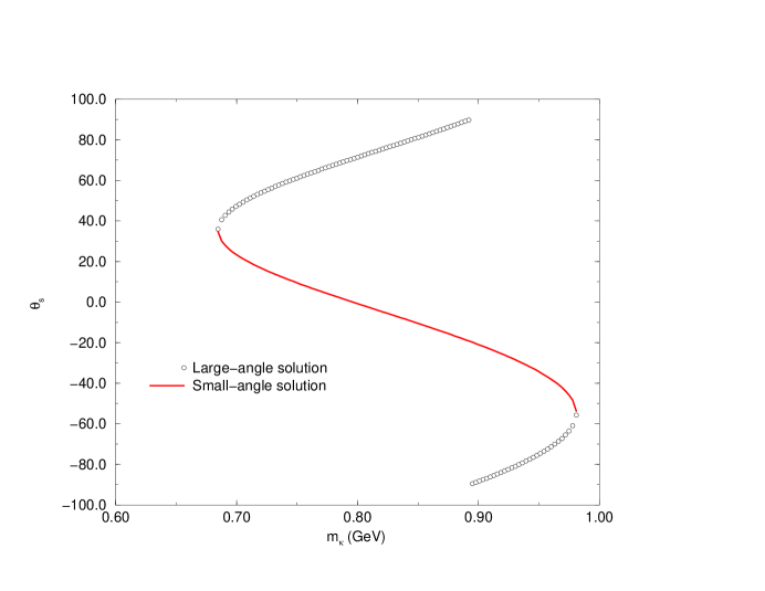
FIG. 1.: Scalar mixing angle solutions as functions of $m_{\kappa}$.

Next let us consider the trilinear scalar-pseudoscalar-pseudoscalar interaction which is related to the main decay modes of the light scalar nonet states. We denote the matrix of pseudoscalar nonet fields by $\phi_{a}^{b}\left(x\right)$. The general $SU\left(3\right)$ flavor invariant $N\phi\phi$ interaction is written as

$${\cal L}_{N\phi\phi}=A{\epsilon}^{abc}{\epsilon}_{def}N_{a}^{d}{\partial_{\mu}}{\phi}_{b}^{e}{\partial_{\mu}}{\phi}_{c}^{f} + B{\rm Tr}\left(N\right){\rm Tr}\left({\partial_{\mu}}\phi{\partial_{\mu}}\phi\right)+C{\rm Tr}\left(N{\partial_{\mu}}\phi\right){\rm Tr}\left({\partial_{\mu}}\phi\right)$$ (26)

$$+ D{\rm Tr}\left(N\right){\rm Tr}\left({\partial_{\mu}}\phi\right){\rm Tr}\left({\partial_{\mu}}\phi\right),$$ (27)

where $A,B,C,D$ are four real constants. The derivatives of the pseudoscalars were introduced in order that (27) properly follows from a chiral invariant Lagrangian in which the field $\phi_{a}^{b}$ transforms non-linearly under axial transformations. The chiral aspect of our model is largely irrelevant to the discussion in the present paper but, for completeness, will be briefly treated in Appendix B.

Notice that the first term of (27) may be rewritten as

$$2A{\rm Tr}\left(N{\partial_{\mu}}{\phi}{\partial_{\mu}}{\phi}\right)-A{\rm Tr}\left(N\right){\rm Tr}\left({\partial_{\mu}}\phi{\partial_{\mu}}\phi\right) - 2A{\rm Tr}\left(N{\partial_{\mu}}\phi\right){\rm Tr}\left({\partial_{\mu}}\phi\right)$$ (28)

$$+ A{\rm Tr}\left(N\right){\rm Tr}\left({\partial_{\mu}}\phi\right){\rm Tr}\left({\partial_{\mu}}\phi\right).$$ (29)

Thus, if desired, the complicated looking first term of (27) may be eliminated in favor of the most standard form ${\rm Tr}\left(N{\partial_{\mu}}{\phi}{\partial_{\mu}}{\phi}\right)$. Our motivation for presenting it in the way shown is that, by itself, the first term of (27) predicts zero coupling constants for both $f_{0}\rightarrow\pi\pi$ and $\sigma\rightarrow K\bar{K}$ when the “dual” ideal mixing identifications, $\sigma=N_{3}^{3}$ and $f_{0}=(N_{1}^{1}+N_{2}^{2})/{\sqrt{2}}$, are made. This is in agreement with Jaffe’s picture (see Section VB of [24]) of the dominant scalar decays arising as the “falling apart” or “quark rearrangement” of their constituents. It is easy to see from (8) that $N_{3}^{3}$ cannot fall apart into $K\bar{K}$ and that $(N_{1}^{1}+N_{2}^{2})/{\sqrt{2}}$ cannot fall apart into $\pi\pi$.

Of course $f_{0}\rightarrow\pi\pi$ must be non-zero because $f_{0}(980)$ is observed in $\pi\pi$ scattering. In fact it also vanishes with just the term ${\rm Tr}\left(N\partial_{\mu}\phi\partial_{\mu}\phi\right)$ and the “conventional” identification $\sigma=(N_{1}^{1}+N_{2}^{2})/{\sqrt{2}}$ and $f_{0}=N_{3}^{3}$. Our model contains two sources for $f_{0}\rightarrow\pi\pi$: the deviation from ideal mixing due to the $c$ and $d$ terms in (10) and also the presence of more than one term in (27). Note again that the use of (10) and (27) does not require us to make any commitment as to the quark substructure of $N_{a}^{b}$.

Using isotopic spin invariance, the trilinear $N\phi\phi$ interaction resulting from (27) must have the form

$$-{\cal L}_{N\phi\phi} = \frac{\gamma_{\kappa K\pi}}{\sqrt{2}}\left(\partial_{\mu}{\bar{K}}\mbox{\boldmath${\tau}$}\cdot\partial_{\mu}{\mbox{\boldmath${\pi}$}}\kappa+h.c.\right)+\frac{\gamma_{\sigma\pi\pi}}{\sqrt{2}}\sigma\partial_{\mu}\mbox{\boldmath${\pi}$}\cdot\partial_{\mu}{\mbox{\boldmath${\pi}$}}$$ (30)

$$+ \frac{\gamma_{\sigma KK}}{\sqrt{2}}\sigma\partial_{\mu}{\bar{K}}\partial_{\mu}{K}+\frac{\gamma_{f_{0}\pi\pi}}{\sqrt{2}}f_{0}\partial_{\mu}\mbox{\boldmath${\pi}$}\cdot\partial_{\mu}\mbox{\boldmath${\pi}$}+\frac{\gamma_{f_{0}KK}}{\sqrt{2}}f_{0}\partial_{\mu}{\bar{K}}\partial_{\mu}{K}$$ (31)

$$+ \frac{\gamma_{a_{0}KK}}{\sqrt{2}}\partial_{\mu}{\bar{K}}\mbox{\boldmath${\tau}$}\cdot{\bf a_{0}}\partial_{\mu}{K}+\gamma_{\kappa{K}\eta}\left({\bar{\kappa}}\partial_{\mu}K\partial_{\mu}{\eta}+h.c.\right)+\gamma_{\kappa{K}\eta^{\prime}}\left({\bar{\kappa}}\partial_{\mu}K\partial_{\mu}{\eta^{\prime}}+h.c.\right)$$ (32)

$$+ \gamma_{a_{0}\pi\eta}{\bf a_{0}}\cdot\partial_{\mu}\mbox{\boldmath${\pi}$}\partial_{\mu}\eta+\gamma_{a_{0}\pi\eta^{\prime}}{\bf a_{0}}\cdot\partial_{\mu}\mbox{\boldmath${\pi}$}\partial_{\mu}\eta^{\prime}$$ (33)

$$+ \gamma_{\sigma\eta\eta}\sigma\partial_{\mu}\eta\partial_{\mu}\eta+\gamma_{\sigma\eta\eta^{\prime}}\sigma\partial_{\mu}\eta\partial_{\mu}\eta^{\prime}+\gamma_{\sigma\eta^{\prime}\eta^{\prime}}\sigma\partial_{\mu}\eta^{\prime}\partial_{\mu}\eta^{\prime}$$ (34)

$$+ \gamma_{f_{0}\eta\eta}f_{0}\partial_{\mu}\eta\partial_{\mu}\eta+\gamma_{f_{0}\eta\eta^{\prime}}f_{0}\partial_{\mu}\eta\partial_{\mu}\eta^{\prime}+\gamma_{f_{0}\eta^{\prime}\eta^{\prime}}f_{0}\partial_{\mu}\eta^{\prime}\partial_{\mu}\eta^{\prime},$$ (35)

where the $\gamma$’s are the coupling constants. The fields which appear in this expression are the isomultiplets:

$$K=\left(\begin{array}[]{c}K^{+}\\ K^{0}\end{array}\right),\quad{\bar{K}}=\left(\begin{array}[]{cc}K^{-}&{\bar{K}^{0}}\end{array}\right) \quad\kappa=\left(\begin{array}[]{c}\kappa^{+}\\ \kappa^{0}\end{array}\right),\quad{\bar{\kappa}}=\left(\begin{array}[]{cc}{\kappa}^{-}&{\bar{\kappa}^{0}}\end{array}\right),$$ , (42)

$$\pi^{\pm}=\frac{1}{\sqrt{2}}\left(\pi_{1}\mp i\pi_{2}\right) \quad\pi^{0}=\pi_{3},$$ , (43)

$$a_{0}^{\pm}=\frac{1}{\sqrt{2}}\left(a_{01}\mp ia_{02}\right) \quad a_{0}^{0}=a_{03},$$ , (44)

in addition to the isosinglets $\sigma$, $f_{0}$, $\eta$ and $\eta^{\prime}$. The expressions for the $\gamma$’s in terms of the parameters $A$, $B$, $C$ and $D$ as well as the scalar and pseudoscalar mixing angles are listed, together with some related material, in Appendix C. Notice that if we restrict attention to those terms in which neither an $\eta$ nor an $\eta^{\prime}$ appear [first six terms of (35)], their coupling constants only involve two parameters $A$ and $B$. These are the terms which will be needed for the subsequent work in the present paper.

IV Testing the model’s coupling constant predictions

Now let us consider how well the five coupling constants $\gamma_{\kappa{K}\pi}$, $\gamma_{\sigma\pi\pi}$, $\gamma_{\sigma KK}$, $\gamma_{f_{0}\pi\pi}$ and $\gamma_{f_{0}KK}$, can be correlated in terms of the two parameters $A$ and $B$. These coupling constants, which are listed in Eqs. (C4-C8) are the ones which are relevant for the discussions of $\pi\pi$ scattering given in [2] and $\pi K$ scattering given in [3].

A very important question concerns the way in which these $\gamma$’s are to be related to experiment. For an “isolated” narrow resonance the magnitude of the coupling constant is proportional to the square root of the width. Actually, the only one of the five for which this prescription roughly applies is $\gamma_{f_{0}\pi\pi}$; the appropriate formula is given in Eq. (4.5) of [2]. Even here there is a practical ambiguity in that, while the $\pi\pi$ branching ratio is listed in [22], the total width is uncertain in the range $40-100$MeV. The determination $\left|\gamma_{f_{0}\pi\pi}\right|=2.43$ ${\rm GeV}^{-1}$ given in [2] is based on using $\Gamma_{tot}\left(f_{0}\right)$ as a parameter in the model analysis of $\pi\pi$ scattering and making a best fit.

The situation for $\gamma_{f_{0}KK}$ is somewhat similar due to the poorly determined $\Gamma_{tot}\left(f_{0}\right)$. There is an additional difficulty since the central value of the $f_{0}(980)$ mass is below the $K\bar{K}$ threshold. Thus the value $\left|\gamma_{f_{0}KK}\right|\approx 10$ ${\rm GeV}^{-1}$ presented in Section V of [2], is based on a model taking the finite width of the initial state into account. Incidentally, the non-negligible branching ratio for $f_{0}\rightarrow K\bar{K}$ in spite of the unfavorable phase space is an indication that the $f_{0}$ “wavefunction” has an important piece containing $s\bar{s}$.

The $\sigma$, as “seen” from the analysis of [2], for example, is neither isolated nor narrow. A suitable regularization of the tree amplitude near the $\sigma$ pole was argued to be of the form:

$$\frac{m_{\sigma}G}{m_{\sigma}^{2}-s}\rightarrow\frac{m_{\sigma}G}{m_{\sigma}^{2}-s-im_{\sigma}G^{\prime}},$$ (45)

where $G$ and $G^{\prime}$ are real. G is taken to be proportional to $\gamma_{\sigma\pi\pi}^{2}$ while $G^{\prime}$ is considered to be a regularization parameter. For a narrow resonance with negligible background it would be expected that $G^{\prime}=G$. However, considering both G and $G^{\prime}$ as quantities to be fit (or essentially equivalently, restoring local unitarity in a crossing symmetric way) yields $G^{\prime}\neq G$. The determination $\left|\gamma_{\sigma\pi\pi}\right|=7.81$ ${\rm GeV}^{-1}$ is based on such a fit.

The situation concerning $\gamma_{\kappa{K}\pi}$ is similar to the one for $\gamma_{\sigma\pi\pi}$. Making an analogous fit to the $\displaystyle{I=\frac{1}{2}}$ amplitude of $\pi K$ scattering (see Section IV of [3]) yields $\left|\gamma_{\kappa{K}\pi}\right|\approx 5$ ${\rm GeV}^{-1}$. This value, however, is based on inputting the $\left|\gamma_{f_{0}\pi\pi}\right|$, $\left|\gamma_{f_{0}KK}\right|$ and $\left|\gamma_{\sigma\pi\pi}\right|$ values obtained as above and making a particular choice of $\gamma_{\sigma KK}$. The value of $\gamma_{\sigma KK}$ was however not very accurately determined in this model; a compromise choice was $\gamma_{\sigma KK}\approx 8\>{\rm GeV}^{-1}$.

A summary of the coupling constants previously obtained is shown in Table I.

coupling constant	value (${\rm GeV}^{-1}$)	obtained from
$\left|\gamma_{f_{0}\pi\pi}\right|$	2.4	$\pi\pi$ scattering
$\left|\gamma_{f_{0}KK}\right|$	$\approx 10$	$\pi\pi$ scattering
$\left|\gamma_{\sigma\pi\pi}\right|$	7.8	$\pi\pi$ scattering
$\left|\gamma_{\kappa K\pi}\right|$	5.0	$\pi K$ scattering
$\gamma_{\sigma KK}$	$\approx 8$	$\pi K$ scattering

TABLE I.: Coupling constants previously obtained in [2] and [3].

The discussion above illustrates that it seems necessary to obtain the coupling constants of the low-lying scalars from a detailed consideration of the relevant scattering processes. It is not sufficient to read them off from [22] at the present time. Furthermore their interpretation is linked to the dynamical model from which they are obtained.

It seems to us that a relatively clean way to test the correlation between the coupling constants in Table I is to recalculate the $\pi K$ scattering amplitude and, instead of taking $\left|\gamma_{f_{0}\pi\pi}\right|$, $\left|\gamma_{f_{0}KK}\right|$ and $\left|\gamma_{\sigma\pi\pi}\right|$ from the $\pi\pi$ scattering output and regarding $\gamma_{\kappa{K}\pi}$ and $\gamma_{\sigma KK}$ as fitting parameters as in [3], just $A$ and $B$ are now taken to be fitted.

We work within the same theoretical framework that was developed in [2] for the $\pi\pi$ scattering analysis and was further explored in [3] for the case of $\pi K$ scattering. In this framework, the $\pi K$ scattering amplitude is computed in a model motivated by the ${1}/{N_{c}}$ picture of QCD and its real part is given as a sum of regularized tree level graphs which include all resonances that contribute to the amplitude up to the energy region of interest. The relevant Feynman diagrams are shown in Fig. 1 of [3].

In the $\displaystyle{I=\frac{1}{2}}$ channel, we perform a $\chi^{2}$ fit, using the MINUIT package, of this model to the experimental data. Specifically, in addition to $A$ and $B$, the parameters to be fit are the regularization parameter in the $\kappa$ propagator, $G^{\prime}_{\kappa}$ (which can also be interpreted as a total $\kappa$ decay width), and parameters of the resonance $K_{0}^{*}(1430)$: its mass $M_{*}$, its coupling $\gamma_{*}$ and the regularization parameter in its s-channel propagator $G^{\prime}_{*}$. This will be done for different choices of $m_{\kappa}$. Note that the scalar mixing angle $\theta_{s}$ (see Section III) will be different for each choice of $m_{\kappa}$. In fact, as already discussed, this actually gives two different mixing angles for each $m_{\kappa}$, one (large angle solution) closer to the $q\bar{q}$ ansatz (6) and the other (small angle solution) closer to the $qq\bar{q}\bar{q}$ ansatz (8). It is very interesting to see which one is chosen in our model. More details of the model are given in [3]. The possible values of $m_{\kappa}$ are limited by (22) for consistency with our present model for masses based on Eq. (10).

Let us first choose $m_{\kappa}=897$MeV, as obtained in [3]. Then the fit to the real part of the $\displaystyle{I=\frac{1}{2}}$ amplitude, ${\rm R}_{0}^{\frac{1}{2}}$ is shown in Fig. 2 while the fitted parameters and resulting predicted coupling constants are given in Table II. The results for both possible mixing angles corresponding to $m_{\kappa}=897$MeV are included. It is seen that the $\chi^{2}$ fits to ${\rm R}_{0}^{\frac{1}{2}}$ are essentially equally good compared to each other and compared to the one in [3]. However if we compare the coupling constants in Table II with those obtained previously in Table I we see that while the coupling constants $\gamma_{f_{0}\pi\pi}$, $\gamma_{f_{0}KK}$, $\gamma_{\sigma\pi\pi}$ and $\gamma_{\kappa K\pi}$ obtained with $\theta_{s}\approx-20^{\circ}$ agree with those obtained earlier in connection with $\pi\pi$ and $\pi K$ scattering, their values obtained with $\theta_{s}\approx-89^{\circ}$ do not agree so well.

Furthermore the value of $\gamma_{f_{0}\pi\pi}$ obtained with $\theta_{s}\approx-89^{\circ}$ would lead to a value for the $f_{0}$ width several times larger than the experimentally allowed range. It thus seems that the $qq\bar{q}\bar{q}$ picture, to which $\theta_{s}\approx-17^{\circ}$ is much closer, gives a better overall description of the scalar nonet than does the $q\bar{q}$ picture.

It is interesting to investigate the effect of changing $m_{\kappa}$ within the range given in Eq. (22). As examples, Tables III and IV show the fitted parameters for $m_{\kappa}=875$ MeV and $m_{\kappa}=800$ MeV respectively. Several trends can be discerned. As $m_{\kappa}$ decreases from 897 MeV the goodness of fit actually improves from $\chi^{2}=3.94$ to $\chi^{2}=2.3$ at $m_{\kappa}=800$ MeV. On the other hand the value of $\gamma_{f_{0}\pi\pi}$ increases so that at $m_{\kappa}=875$ MeV the $f_{0}\rightarrow\pi\pi$ width is in slightly better agreement with experiment and at $m_{\kappa}=800$ MeV it is many times larger than allowed by experiment. It seems that the fit at $m_{\kappa}=875$ MeV is not very different from the one at $m_{\kappa}=897$ MeV; this gives an estimate of the “theoretical uncertainty” in our calculation. On the other hand $m_{\kappa}=800$ MeV seems to be ruled out, as are still lower values of $m_{\kappa}$.

Another argument in favor of the larger values of $m_{\kappa}$ can be made by examining the $\displaystyle{I=\frac{3}{2}}$ $\pi K$ amplitude , shown in Fig. 3. It is seen that decreasing $m_{\kappa}$ worsens the agreement with experiment. This feature arises because $\gamma_{\sigma KK}$, to which the $\displaystyle{I=\frac{3}{2}}$ amplitude is sensitive, increases with decreasing $m_{\kappa}$. This situation was discussed in more detail in section V of [3], where it was noted that higher mass resonances may be important in this channel.

We note that the three parameters describing the $K_{0}^{*}(1430)$ are stable to varying $m_{\kappa}$.

All the fits yield for the parameters $A$ and $B$ that $\frac{B}{A}{>}\!\!\!\!{{}_{\sim}}-1$. Using (27) then shows that ${\cal L}_{N\phi\phi}$ approximately looks like

$${\cal L}_{N\phi\phi}\approx 2A\left[{\rm Tr}\left(N\partial_{\mu}\phi\partial_{\mu}\phi\right)-\rho{\rm Tr}\left(N\right){\rm Tr}\left(\partial_{\mu}\phi\partial_{\mu}\phi\right)\right]+\cdot\cdot\cdot,$$ (46)

where $\rho$ is a positive number slightly less than unity and the three dots stand for the $C$ and $D$ terms which only contribute to vertices involving at least one $\eta$ or $\eta^{\prime}$.

Using this model we can also estimate the partial decay width of $a_{0}(980)\rightarrow K{\bar{K}}$ which is entirely determined in terms of the parameter $A$ [see Eq.(C4)]. As in the case of $f_{0}(980)$, the resonance lies below the decay threshold so the effect of the finite width of the decaying state must be taken into account [see for example footnote 2 of [2]]. The results are shown in Table V (taking $m_{\kappa}=897$ MeV) corresponding to the extremes of the total width range given in [22]. Also the effect of the mass difference between the charged and neutral kaons is taken into account. The numerical values seem reasonable.

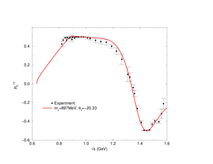
FIG. 2.: Comparison of the theoretical prediction of $R_{0}^{1/2}$ with its experimental data.

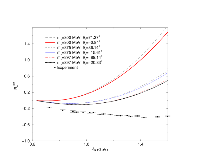
FIG. 3.: Comparison of the theoretical predictions of $R_{0}^{3/2}$ with its experimental data.

$\begin{array}[]{|c|c|c|}\hline\cr{\rm Fitted\hskip 5.69046ptParameter}&{\rm\theta_{s}=-20.33}&{\rm\theta_{s}=-89.14}\\ \hline\cr G^{\prime}_{\kappa}&314\pm 3\>{\rm MeV}&322\pm 3\>{\rm MeV}\\ \hline\cr M_{*}&1390\pm 4\>{\rm MeV}&1389\pm 4\>{\rm MeV}\\ \hline\cr\gamma_{*}&4.42\pm 0.09\>{\rm GeV}^{-1}&4.4\pm 0.09\>{\rm GeV}^{-1}\\ \hline\cr G^{\prime}_{*}&275\pm 10\>{\rm MeV}&273\pm 11\>{\rm MeV}\\ \hline\cr A&2.51\pm 0.03\>{\rm GeV}^{-1}&2.57\pm 0.03\>{\rm GeV}^{-1}\\ \hline\cr B&-1.95\pm 0.04\>{\rm GeV}^{-1}&-2.12\pm 0.04\>{\rm GeV}^{-1}\\ \hline\cr\chi^{2}&3.94&3.95\\ \hline\cr\vrule\lx@intercol\hfil{\rm Predicted\hskip 5.69046ptCouplings}\hfil\lx@intercol\vrule\lx@intercol\\ \hline\cr\gamma_{\kappa K\pi}&-5.02\>{\rm GeV}^{-1}&-5.14\>{\rm GeV}^{-1}\\ \hline\cr\gamma_{\sigma\pi\pi}&7.26\>{\rm GeV}^{-1}&4.33\>{\rm GeV}^{-1}\\ \hline\cr\gamma_{f\pi\pi}&1.46\>{\rm GeV}^{-1}&-6.56\>{\rm GeV}^{-1}\\ \hline\cr\gamma_{\sigma KK}&9.62\>{\rm GeV}^{-1}&13.69\>{\rm GeV}^{-1}\\ \hline\cr\gamma_{fKK}&10.10\>{\rm GeV}^{-1}&-5.78\>{\rm GeV}^{-1}\\ \hline\cr\end{array}$

TABLE II.: Extracted parameters from a fit to the $\pi K$ data. $m_{\kappa}=897$ MeV.

$\begin{array}[]{|c|c|c|}\hline\cr{\rm Fitted\hskip 5.69046ptParameter}&{\rm\theta_{s}=-15.61}&{\rm\theta_{s}=86.14}\\ \hline\cr G^{\prime}_{\kappa}&346\pm 2\>{\rm MeV}&357\pm 3\>{\rm MeV}\\ \hline\cr M_{*}&1389\pm 4\>{\rm MeV}&1388\pm 4\>{\rm MeV}\\ \hline\cr\gamma_{*}&4.42\pm 0.09\>{\rm GeV}^{-1}&4.39\pm 0.09\>{\rm GeV}^{-1}\\ \hline\cr G^{\prime}_{*}&275\pm 10\>{\rm MeV}&272\pm 10\>{\rm MeV}\\ \hline\cr A&2.87\pm 0.03\>{\rm GeV}^{-1}&2.96\pm 0.03\>{\rm GeV}^{-1}\\ \hline\cr B&-2.34\pm 0.03\>{\rm GeV}^{-1}&-2.56\pm 0.04\>{\rm GeV}^{-1}\\ \hline\cr\chi^{2}&3.23&3.26\\ \hline\cr\vrule\lx@intercol\hfil{\rm Predicted\hskip 5.69046ptCouplings}\hfil\lx@intercol\vrule\lx@intercol\\ \hline\cr\gamma_{\kappa K\pi}&-5.75\>{\rm GeV}^{-1}&-5.92\>{\rm GeV}^{-1}\\ \hline\cr\gamma_{\sigma\pi\pi}&8.36\>{\rm GeV}^{-1}&-4.58\>{\rm GeV}^{-1}\\ \hline\cr\gamma_{f\pi\pi}&2.53\>{\rm GeV}^{-1}&8.13\>{\rm GeV}^{-1}\\ \hline\cr\gamma_{\sigma KK}&10.45\>{\rm GeV}^{-1}&-15.62\>{\rm GeV}^{-1}\\ \hline\cr\gamma_{fKK}&12.76\>{\rm GeV}^{-1}&8.30\>{\rm GeV}^{-1}\\ \hline\cr\end{array}$

TABLE III.: Extracted parameters from a fit to the $\pi K$ data. $m_{\kappa}=875$ MeV.

$\begin{array}[]{|c|c|c|}\hline\cr{\rm Fitted\hskip 5.69046ptParameter}&{\rm\theta_{s}=-0.84}&{\rm\theta_{s}=71.37}\\ \hline\cr G^{\prime}_{\kappa}&450\pm 2\>{\rm MeV}&479\pm 2\>{\rm MeV}\\ \hline\cr M_{*}&1387\pm 4\>{\rm MeV}&1384\pm 4\>{\rm MeV}\\ \hline\cr\gamma_{*}&4.40\pm 0.09\>{\rm GeV}^{-1}&4.36\pm 0.09\>{\rm GeV}^{-1}\\ \hline\cr G^{\prime}_{*}&273\pm 10\>{\rm MeV}&268\pm 11\>{\rm MeV}\\ \hline\cr A&4.32\pm 0.03\>{\rm GeV}^{-1}&4.50\pm 0.04\>{\rm GeV}^{-1}\\ \hline\cr B&-3.91\pm 0.03\>{\rm GeV}^{-1}&-4.29\pm 0.04\>{\rm GeV}^{-1}\\ \hline\cr\chi^{2}&2.34&2.39\\ \hline\cr\vrule\lx@intercol\hfil{\rm Predicted\hskip 5.69046ptCouplings}\hfil\lx@intercol\vrule\lx@intercol\\ \hline\cr\gamma_{\kappa K\pi}&-8.64\>{\rm GeV}^{-1}&-9.01\>{\rm GeV}^{-1}\\ \hline\cr\gamma_{\sigma\pi\pi}&11.76\>{\rm GeV}^{-1}&-4.15\>{\rm GeV}^{-1}\\ \hline\cr\gamma_{f\pi\pi}&7.65\>{\rm GeV}^{-1}&14.52\>{\rm GeV}^{-1}\\ \hline\cr\gamma_{\sigma KK}&11.41\>{\rm GeV}^{-1}&-20.91\>{\rm GeV}^{-1}\\ \hline\cr\gamma_{fKK}&24.12\>{\rm GeV}^{-1}&19.85\>{\rm GeV}^{-1}\\ \hline\cr\end{array}$

TABLE IV.: Extracted parameters from a fit to the $\pi K$ data. $m_{\kappa}=800$ MeV.

decay widths	$\Gamma_{a_{0}}^{tot}=50\>{\rm MeV}$	$\Gamma_{a_{0}}^{tot}=100\>{\rm MeV}$
$\Gamma{\left({a_{0}^{0}}\rightarrow{K^{0}\bar{K^{0}}}\right)}$	0.924 MeV	2.049 MeV
$\Gamma\left(a_{0}^{0}\rightarrow K^{+}K^{-}\right)$	1.371 MeV	2.455 MeV

TABLE V.: Predicted $a_{0}\rightarrow K\bar{K}$ decay widths

V Discussion

We studied the family relationship of a possible scalar nonet composed of the $f_{0}(980)$, the $a_{0}(980)$ and the $\sigma$ and $\kappa$ type states found in recent treatments of $\pi\pi$ scattering and $\pi K$ scattering. The investigation was carried out in the effective Lagrangian framework, starting from the notion of “ideal mixing”. First it was observed that Okubo’s original treatment allows two solutions: one the conventional (e.g. vector meson) $q\bar{q}$ type and the other a “dual” picture which is equivalent to Jaffe’s $qq\bar{q}\bar{q}$ model.

The four masses of our scalar nonet candidates have a similar, but not identical pattern to the one expected in the dual ideal mixing picture. In order to allow for a deviation from ideal mixing, we have added more terms to the Lagrangian [see (10)]. The resulting mass, mixing and scalar-pseudoscalar-pseudoscalar coupling patterns [see (27)] were discussed in detail. The outcome of this analysis is that the dual picture is in fact favored. More quantitatively, the appropriate scalar mixing angle in Eq. (23) comes out to be about $-17^{\circ}\pm 4^{\circ}$ compared with $0^{\circ}$ for dual ideal mixing and $\pm 90^{\circ}$ for conventional ideal mixing. This corresponds to $m_{\kappa}$ ranging from $865-900$ MeV.

The coupling constant results obtained here may be useful for a number of applications in low energy hadron phenomenology. These are defined in Eq. (35) and listed in Appendix C. Typical values of $A$ and $B$ may be read from the small magnitude angle solution in Tables II and III. We expect to improve and further check the accuracy of this model by extending the underlying models of $\pi\pi$ and $\pi K$ scattering to higher energies and to other channels. Finally, it may be interesting to compare our results with those of quark model and lattice gauge theory approaches to QCD.

A Diagonalization of Hyperfine Hamiltonian

In this Appendix, we give some explicit details of the derivation of (13) and (14) which, while not being explicitly used in our approach, furnish the main reason for expecting the scalar $qq\bar{q}\bar{q}$ states to be especially strongly bound. Our results agree with those of Jaffe who followed a different method.

Let us begin by considering only flavor quantum numbers in order to write down the quark content of members of a $qq\bar{q}\bar{q}$ scalar nonet. Taking the quarks to be in the fundamental representation, $\bf{3}$, of $SU(3)_{f}$ we have the familiar irreducible decomposition of products of quark states:

$${\bf{3}}\bigotimes{\bf{3}}={\bf{6}}\bigoplus{\bf{\bar{3}}}$$ (A1)

$${\bf{\bar{3}}}\bigotimes{\bf{\bar{3}}}={\bf{\bar{6}}}\bigoplus{\bf{3}}.$$ (A2)

So the only possibility for obtaining a $qq\bar{q}\bar{q}$ flavor nonet is from the combination $\displaystyle{{\bf{\bar{3}}}\bigotimes{\bf{3}}}$ of $q^{2}\bigotimes{{\bar{q}}^{2}}$ states. Let $q_{i}$ be a basis for the representation space ${\bf{3}}$, where i=1,2 and 3 correspond to up, down and strange quarks respectively, with conjugate (antiquark) basis ${\bar{q}}^{i}$. Then we can consider “dual quark” bases corresponding to the $qq$ and $\bar{q}\bar{q}$ flavor triplet spaces (thus the states are antisymmetric with respect to exchange of flavor indices), namely $T_{m}:=\epsilon_{mjk}{\bar{q}}^{j}{\bar{q}}^{k}$ and $T^{m}:=\epsilon^{mjk}q_{j}q_{k}$. Up to (anti)symmeterization and linear combinations we have the flavor nonet given in Eq. (8). Since $T^{m}$ and $T_{m}$ contain at most one strange quark each the nonet states contain at most two strange quarks. We note also that, in contrast to the conventional $q\bar{q}$ scalar nonet, $N_{3}^{3}$ is non-strange in this realization.

In order to complete the description of $qq\bar{q}\bar{q}$ scalar nonets we consider the spin and color quantum numbers. Using the facts that (i) the $qq$ and $\bar{q}\bar{q}$ parts of the state are individually totally antisymmetric and (ii) the overall $qq\bar{q}\bar{q}$ hadron must be a color singlet, where the quarks transform according to the fundamental representation of $SU(3)_{c}$, we obtain just two possibilities which include scalar flavor nonets (noting that ${\bf{6_{c}}}\bigotimes{\bf{{\bar{6}}_{c}}}={\bf 1_{c}}\bigoplus{\bf{8_{c}}}\bigoplus{\bf{27_{c}}}$), namely

$${|0^{+},{\bf 9}\rangle}_{1}:={\left[0^{+},{\bf{\bar{3}}_{f}},{\bf{\bar{3}}_{c}}\right]}_{qq}\bigotimes{\left[0^{+},{\bf{3_{f}}},{\bf{3_{c}}}\right]}_{\bar{q}\bar{q}}$$ (A3)

$${|0^{+},{\bf 9}\rangle}_{2}:={\left[1^{+},{\bf{\bar{3}}_{f}},{\bf{6_{c}}}\right]}_{qq}\bigotimes{\left[1^{+},{\bf{3_{f}}},{\bf{\bar{6}}_{c}}\right]}_{\bar{q}\bar{q}},$$ (A4)

where we have shown the spin-parity, flavor and color representations respectively for $qq$ and $\bar{q}\bar{q}$ separately.

The “hyperfine” interaction Hamiltonian needed for our discussion is given in Eq. (11).

Given two representations of SU(n) we have the well-known relationship between the quadratic Casimirs of these representations, say ${{\bf J}_{A}}^{2}$ and ${{\bf J}_{B}}^{2}$, and that of their product:

$${{\bf J}_{A}}\cdot{{\bf J}_{B}}=\frac{1}{2}\left[{{\bf J}_{total}}^{2}-{{\bf J}_{A}}^{2}-{{\bf J}_{B}}^{2}\right].$$ (A5)

It can be seen, using (A5), that the parts of the hyperfine Hamiltonian which involve sums over $qq$ or $\bar{q}\bar{q}$ pairs are diagonal with respect to the bases for the scalar nonets chosen in (A3) and (A4). In order to calculate the expectation value of the $q\bar{q}$ terms in (11) using (A5) we first expand the bases (A3) and (A4) in terms of states where the spin and color of the $q\bar{q}$ pairs are explicit.

To find the recoupling coefficients we follow Close [28], where more detail is given. For the case of spin recoupling we have, assuming that all of the quarks in the scalar meson are in relative s-wave states, that in order to couple to total angular momentum $J=0$, either both $q\bar{q}$ pairs must be in $j^{P}=1^{-}$ or both in $j^{P}=0^{-}$ states, which we denote as vector, ($V$), and pseudoscalar, ($P$) respectively. Thus we can expand the spin part of the state in the following manner:

$${|J_{total}=0\rangle}_{1\>{\rm or}\>2}=\alpha PP+\beta VV,$$ (A6)

where $\alpha$ and $\beta$ can be determined in each case by rewriting both sides (the left-hand-side will be different for the two states (A3) and (A4)) in terms of their constituent quarks and antiquarks using the usual Clebsch-Gordon identities for $SU(2)$.

Similarly for the color states we note that, since ${\bf 3}\bigotimes{\bf\bar{3}}={\bf 8}\bigoplus{\bf 1}$, only combinations of the form

$${\alpha^{\prime}}|{\bf 8_{c}}\rangle_{q\bar{q}}\bigotimes|{\bf 8_{c}}\rangle_{q\bar{q}}+{\beta^{\prime}}|{\bf 1_{c}}\rangle_{q\bar{q}}\bigotimes|{\bf 1_{c}}\rangle_{q\bar{q}}$$ (A7)

include color singlets and therefore the color parts of (A3) and (A4) can be written in terms of this basis. For brevity we simply present the results of our recoupling coefficient expansions in Table VI.

${\rm nonet}$	${\rm spins\>of}q\bar{q}{\rm\>pairs}$	${\rm color\>products\>of}q\bar{q}{\rm\>pairs}$
${|0^{+},{\bf 9}\rangle}_{1}$	$\frac{1}{2}PP+\frac{\sqrt{3}}{2}VV$	$\frac{1}{\sqrt{3}}{\bf 1}_{c}\bigotimes{\bf 1}_{c}-{\sqrt{\frac{2}{3}}}{\bf 8}_{c}\bigotimes{\bf 8}_{c}$
${|0^{+},{\bf 9}\rangle}_{2}$	$\frac{{\sqrt{3}}}{2}PP-\frac{1}{2}VV$	$\sqrt{\frac{2}{3}}{\bf 1}_{c}\bigotimes{\bf 1}_{c}+{\sqrt{\frac{1}{3}}}{\bf 8}_{c}\bigotimes{\bf 8}_{c}$

TABLE VI.: Spin and color recouplings for flavour nonets

$\begin{array}[]{|c|l|}\hline\cr\hline\cr{\rm{Representation}}&\>{\bf F}^{2}\\ \hline\cr{\bf 3}{\>{\rm or}\>}{\bf\bar{3}}&\frac{4}{3}\\ {\bf 8}&3\\ {\bf 1}&0\\ {\bf 6}&\frac{10}{3}\\ \hline\cr\hline\cr\end{array}$

TABLE VII.: SU(3) Quadratic Casimirs

In order to give an idea of the next step let us look at one of the off-diagonal elements of $\langle H_{hf}\rangle$, where $H_{hf}$ is as in (11), with respect to the basis given in (A3) and (A4). Labelling the quarks/antiquarks $q_{1}q_{2}{\bar{q}}_{3}{\bar{q}}_{4}$ we have that the only non-vanishing off-diagonal pieces in $\langle H_{hf}\rangle$ are the sums over $(13)$, $(14)$, $(23)$ and $(24)$. For example, applying (A5) yields

$${\bf S_{1}\cdot S_{3}F_{1}\cdot F_{3}}|0^{+},{\bf 9_{f}}\rangle_{1}=\frac{1}{2}\left[-{{\frac{6}{4}\cdot\frac{1}{2}}}PP+{{\frac{1}{2}\cdot\frac{\sqrt{3}}{2}}}VV\right]\left[{{-\frac{8}{3}\cdot\frac{1}{\sqrt{3}}}}{\bf 1_{c}}\bigotimes{\bf 1_{c}}-{{\frac{1}{3}\cdot\sqrt{\frac{2}{3}}}}{\bf 8_{c}}\bigotimes{\bf 8_{c}}\right],$$ (A8)

where for the color operators we have used the $SU(3)$ Casimirs given in Table VII. Finally we take the inner product with the expansion of ${|0^{+},{\bf 9}\rangle}_{2}$ in Table VI which gives that

$$\langle{\bf S_{1}\cdot S_{3}F_{1}\cdot F_{3}}\rangle_{21}=\frac{1}{4}\sqrt{\frac{3}{2}}.$$ (A9)

There are, as noted above, four such combinations, all of which contribute equally. An analogous calculation can be performed for the diagonal matrix elements giving finally:

$$\langle H_{hf}\rangle_{ab}=-\Delta\left[\begin{array}[]{c c}1&\sqrt{\frac{3}{2}}\\ \sqrt{\frac{3}{2}}&\frac{11}{6}\end{array}\right],$$ (A10)

where a and b run over the indices 1 and 2 labelling the flavor nonets ${|0^{+},{\bf 9}\rangle}_{1}$ and ${|0^{+},{\bf 9}\rangle}_{2}$. Thus the eigenstates of the hyperfine interaction correspond to mixtures of these nonets, corresponding to energies $E_{1}=-2.71\Delta$ and $E_{2}=-0.12\Delta$, which are in agreement with [24]. The corresponding eigenstates are:

$${|0^{+},{\bf 9}\rangle} = 0.585{|0^{+},{\bf 9}\rangle}_{1}+0.811{|0^{+},{\bf 9}\rangle}_{2}$$ (A11)

$${|0^{+},{\bf 9}^{*}\rangle} = 0.811{|0^{+},{\bf 9}\rangle}_{1}-0.585{|0^{+},{\bf 9}\rangle}_{2}.$$ (A12)

B Chiral Covariant Form

Here we present the terms of the total Lagrangian involving the scalar nonet $N_{a}^{b}(x)$ in chiral invariant or (for the mass terms which break the chiral symmetry) in chiral covariant form. We follow the general method of non-linear realization described in [27] but our notation is as in Appendix B of [3]. The object $\xi={\rm exp}(i\phi/F_{\pi})$ discussed there transforms as

$$\xi\rightarrow U_{L}\xi K^{\dagger}=K\xi U_{R}^{\dagger}$$ (B1)

under chiral transformation. Our nonet field is considered to transform as if it were made of “constituent” quarks, namely

$$N\rightarrow KNK^{\dagger}.$$ (B2)

With the convenient objects

$$p_{\mu}={i\over 2}\left(\xi\partial_{\mu}\xi^{\dagger}-\xi^{\dagger}\partial_{\mu}\xi\right)\hskip 14.22636pt,\hskip 14.22636ptv_{\mu}={i\over 2}\left(\xi\partial_{\mu}\xi^{\dagger}+\xi^{\dagger}\partial_{\mu}\xi\right)$$ (B3)

we write the additional Lagrangian terms involving $N$:

$${\cal L} = -{1\over 2}{\rm Tr}\left({\cal D}_{\mu}N{\cal D}_{\mu}N\right)-a{\rm Tr}(NN)-{b\over 2}{\rm Tr}\left[NN\left(\xi^{\dagger}{\cal M}\xi^{\dagger}+\xi{{\cal M}}^{\dagger}\xi\right)\right]-c{\rm Tr}(N){\rm Tr}(N)$$ (B4)

$$- {d\over 2}{\rm Tr}(N){\rm Tr}\left[N\left(\xi^{\dagger}{\cal M}\xi^{\dagger}+\xi{{\cal M}^{\dagger}}\xi\right)\right]+F_{\pi}^{2}\left[A\epsilon^{abc}\epsilon_{def}N_{a}^{d}(p_{\mu})_{b}^{e}(p_{\mu})_{c}^{f}+B{\rm Tr}(N){\rm Tr}(p_{\mu}p_{\mu})\right.$$ (B5)

$$+ \left.C{\rm Tr}(Np_{\mu}){\rm Tr}(p_{\mu})+D{\rm Tr}(N){\rm Tr}(p_{\mu}){\rm Tr}(p_{\mu})\right]$$ (B6)

where ${\cal D}=\partial_{\mu}-iv_{\mu}$ and ${\cal M}={\cal M}^{\dagger}$ is the spurion matrix defined after (1). The entire Eq.(B6) is formally invariant if we allow ${\cal M}$ to transform as ${\cal M}\rightarrow U_{L}{\cal M}U_{R}^{\dagger}$. This Lagrangian reproduces (10) and (27) but also contain interactions with extra pions. These extra interactions do not change anything in this paper or in the tree-level formulas for $\phi\phi$ scattering in [2] and [3].

C Coupling Constants

Here we find the scalar-pseudoscalar-pseudoscalar coupling constants defined in (35) in terms of the parameters $A,B,C,D$ [see (27)], the scalar mixing angle [see (23)] and the pseudoscalar mixing angle, $\theta_{p}$. The latter is defined according to:

$$\left(\begin{array}[]{c}\eta\\ \eta^{\prime}\end{array}\right)=\left(\begin{array}[]{c c}{\rm cos}\theta_{p}&-{\rm sin}\theta_{p}\\ {\rm sin}\theta_{p}&{\rm cos}\theta_{p}\end{array}\right)\left(\begin{array}[]{c}(\phi^{1}_{1}+\phi^{2}_{2})/\sqrt{2}\\ \phi^{3}_{3}\end{array}\right),$$ (C1)

where $\eta$ and $\eta^{\prime}$ are the fields which diagonalize the pseudoscalar analog of (17). The usual convention employs a different basis; in this convention the angle is $\theta_{u}$ and

$$\left(\begin{array}[]{c}\eta\\ \eta^{\prime}\end{array}\right)=\left(\begin{array}[]{c c}{\rm cos}\theta_{u}&-{\rm sin}\theta_{u}\\ {\rm sin}\theta_{u}&{\rm cos}\theta_{u}\end{array}\right)\left(\begin{array}[]{c}(\phi^{1}_{1}+\phi^{2}_{2}-2\phi^{3}_{3})/\sqrt{6}\\ (\phi^{1}_{1}+\phi^{2}_{2}+\phi^{3}_{3})/\sqrt{6}\end{array}\right).$$ (C2)

The relation between the two angles is

$$\theta_{p}=\theta_{u}+54.74^{o}\approx 37^{o}$$ (C3)

in which case (see for example [32]) $\theta_{u}\approx-18^{o}$ was taken. More recent analyses ([33] and [34]) have modified this treatment somewhat by considering derivative mixing terms as well as non-derivative ones.

Note that the basis for (C1) was chosen so that ${\bar{q}}q$ is the more natural picture for the pseudoscalar nonet, in contrast to (23) for the scalars. Because the mixing angles can take on any values, this in no way biases the analysis one way or the other.

The $\gamma$’s are predicted in the present model as

$$\gamma_{\kappa K\pi} = \gamma_{a_{0}KK}=-2A$$ (C4)

$$\gamma_{\sigma\pi\pi} = 2B{\rm sin}\theta_{s}-\sqrt{2}(B-A){\rm cos}\theta_{s}$$ (C5)

$$\gamma_{\sigma K{K}} = 2(2B-A){\rm sin}\theta_{s}-2\sqrt{2}B{\rm cos}\theta_{s}$$ (C6)

$$\gamma_{f_{0}\pi\pi} = \sqrt{2}(A-B){\rm sin}\theta_{s}-2B{\rm cos}\theta_{s}$$ (C7)

$$\gamma_{f_{0}K{K}} = 2(A-2B){\rm cos}\theta_{s}-2\sqrt{2}B{\rm sin}\theta_{s}$$ (C8)

$$\gamma_{\kappa{K}\eta} = C{\rm sin}\theta_{p}-\sqrt{2}(C-A){\rm cos}\theta_{p}$$ (C9)

$$\gamma_{\kappa{K}\eta^{\prime}} = \sqrt{2}(A-C){\rm sin}\theta_{p}-C{\rm cos}\theta_{p}$$ (C10)

$$\gamma_{a_{0}\pi\eta} = (C-2A){\rm sin}\theta_{p}-\sqrt{2}C{\rm cos}\theta_{p}$$ (C11)

$$\gamma_{a_{0}\pi\eta^{\prime}} = (2A-C){\rm cos}\theta_{p}-\sqrt{2}C{\rm sin}\theta_{p}$$ (C12)

$$\gamma_{\sigma\eta\eta} = \left[\sqrt{2}(B+D)-{1\over 2}(C+2A+4D){\rm sin}2\theta_{p}+\sqrt{2}(C+D){\rm cos}^{2}\theta_{p}\right]{\rm sin}\theta_{s}$$ (C14)

$$-\left[(B+D)-{1\over\sqrt{2}}(C+2D){\rm sin}2\theta_{p}+(A+D){\rm cos}^{2}\theta_{p}+C{\rm sin}^{2}\theta_{p}\right]{\rm cos}\theta_{s}$$

$$\gamma_{\sigma\eta^{\prime}\eta^{\prime}} = \left[\sqrt{2}(B+D)+{1\over 2}(C+2A+4D){\rm sin}2\theta_{p}+\sqrt{2}(C+D){\rm sin}^{2}\theta_{p}\right]{\rm sin}\theta_{s}$$ (C16)

$$-\left[(B+D)+{1\over\sqrt{2}}(C+2D){\rm sin}2\theta_{p}+(A+D){\rm sin}^{2}\theta_{p}+C{\rm cos}^{2}\theta_{p}\right]{\rm cos}\theta_{s}$$

$$\gamma_{\sigma\eta\eta^{\prime}} = \left[\sqrt{2}(C+D){\rm sin}2\theta_{p}+(C+2A+4D){\rm cos}2\theta_{p}\right]{\rm sin}\theta_{s}$$ (C18)

$$-\left[\sqrt{2}(C+2D){\rm cos}2\theta_{p}+(A-C+D){\rm sin}2\theta_{p}\right]{\rm cos}\theta_{s}$$

$$\gamma_{f_{0}\eta\eta} = \left[-\sqrt{2}(B+D)+{1\over 2}(C+2A+4D){\rm sin}2\theta_{p}-\sqrt{2}(C+D){\rm cos}^{2}\theta_{p}\right]{\rm cos}\theta_{s}$$ (C20)

$$-\left[(B+D)-{1\over\sqrt{2}}(C+2D){\rm sin}2\theta_{p}+(A+D){\rm cos}^{2}\theta_{p}+C{\rm sin}^{2}\theta_{p}\right]{\rm sin}\theta_{s}$$

$$\gamma_{f_{0}\eta^{\prime}\eta^{\prime}} = -\left[\sqrt{2}(B+D)+{1\over 2}(C+2A+4D){\rm sin}2\theta_{p}+\sqrt{2}(C+D){\rm sin}^{2}\theta_{p}\right]{\rm cos}\theta_{s}$$ (C22)

$$-\left[(B+D)+{1\over\sqrt{2}}(C+2D){\rm sin}2\theta_{p}+(A+D){\rm sin}^{2}\theta_{p}+C{\rm cos}^{2}\theta_{p}\right]{\rm sin}\theta_{s}$$

$$\gamma_{f_{0}\eta\eta^{\prime}} = -\left[\sqrt{2}(C+D){\rm sin}2\theta_{p}+(C+2A+4D){\rm cos}2\theta_{p}\right]{\rm cos}\theta_{s}$$ (C24)

$$-\left[\sqrt{2}(C+2D){\rm cos}2\theta_{p}+(A-C+D){\rm sin}2\theta_{p}\right]{\rm sin}\theta_{s}$$

REFERENCES

[1]
F. Sannino and J. Schechter, Phys. Rev. D52, 96 (1995).
[2]
M. Harada, F. Sannino and J. Schechter, Phys. Rev. D54, 54
(1996), Phys. Rev. Lett. 78,
1603 (1997).
[3]D. Black, A.H. Fariborz, F. Sannino, and J. Schechter,
Phys. Rev. D58, to be published.
[4] See, for example, N.A. Törnqvist, Z. Phys.
C68, 647 (1995) and references therein. In addition see
N.A. Törnqvist and M. Roos, Phys. Rev. Lett. 76, 1575
(1996).
[5] S. Ishida, M.Y. Ishida, H. Takahashi, T. Ishida,
K. Takamatsu and T Tsuru, Prog. Theor. Phys. 95, 745 (1996).
[6]
D. Morgan and M. Pennington, Phys. Rev. D48, 1185 (1993).
[7]
G. Janssen, B.C. Pearce, K. Holinde and J. Speth, Phys. Rev. D52, 2690 (1995).
[8] A.A. Bolokhov, A.N. Manashov, M.V. Polyakov and
V.V. Vereshagin, Phys. Rev. D48, 3090 (1993). See also
V.A. Andrianov and A.N. Manashov, Mod. Phys. Lett. A8, 2199
(1993). Extension of this string-like approach to the case
has been made in V.V. Vereshagin, Phys. Rev. D55, 5349 (1997)
and very recently in A.V. Vereshagin and V.V. Vereshagin hep-ph/9807399,
which is consistent with a light state.
[10]R. Kamínski, L. Leśniak and J. P. Maillet,
Phys. Rev. D50, 3145 (1994).
[11] M. Svec, Phys. Rev. D53, 2343 (1996).
[12] E. van Beveren, T.A. Rijken, K. Metzger,
C. Dullemond, G. Rupp and J.E. Ribeiro, Z. Phys. C30, 615
(1986).
[13] R. Delbourgo and M.D. Scadron, Mod. Phys. Lett. A10, 251 (1995). See also D. Atkinson, M. Harada and A.I. Sanda,
Phys. Rev. D46, 3884 (1992).
[14] J.A. Oller, E. Oset and J.R. Pelaez, hep-ph/9804209
[15]
S. Ishida, M. Ishida, T. Ishida, K. Takamatsu and T. Tsuru,
Prog. Theor. Phys. 98, 621 (1997). See also M. Ishida and S. Ishida,
Talk given at 7th International Conference on Hadron Spectroscopy (Hadron
97), Upton, NY, 25-30 Aug. 1997, hep-ph/9712231.
[17]A.V. Anisovich and A.V. Sarantsev, Phys. Lett. B413,
137 (1997).
[18]V. Elias, A.H. Fariborz, Fang Shi and T.G. Steele,
Nucl. Phys. A633, 279 (1998).
[19] V. Dmitrasinović, Phys. Rev. C53, 1383 (1996).
[20] E. Witten, Nucl. Phys. B160, 57 (1979). See also
S. Coleman, Aspects of Symmetry, Cambridge University Press
(1985). The original suggestion is given in G. ’t Hooft, Nucl. Phys. B72, 461 (1974).
[21] S. Weinberg, Physica 96A, 327 (1979). J. Gasser
and H. Leutwyler, Ann. of Phys. 158, 142 (1984); J. Gasser and
H. Leutwyler, Nucl. Phys. B250, 465 (1985). A recent review is
given by Ulf-G. Meißner, Rept. Prog. Phys. 56, 903 (1993).
[22]Review of Particle Properties, Phys. Rev. D54 (1996).
[23]S. Okubo, Phys. Lett. 5, 165 (1963).
[24]R.L. Jaffe, Phys. Rev. D15, 267 (1977).
[25]A. Chodos, R. Jaffe, K. Johnson, C. Thorn and V. Weisskopf,
Phys. Rev. D9, 3471 (1974).
[26]N. Isgur and J. Weinstein, Phys. Rev. D41, 2236
(1990).
[27]C. Callan, S. Coleman, J. Wess and B. Zumino,
Phys. Rev. 177, 2247 (1969).
[28] See section 19.3 of F.E. Close, An Introduction to
Quarks and Partons, Academic Press (1979).
[29] See for example M. Harada and J. Schechter,
Phys. Rev. D54, 3394 (1996).
[30]D. Aston et al, Nucl. Phys B296, 493 (1988).
[31]P. Estabrooks et al, Nucl Phys. B133,
490 (1978).
[32]V. Mirelli and J. Schechter, Phys. Rev. D 15, 1361
(1977)
[33]
J. Schechter, A. Subbaraman and H. Weigel, Phys. Rev. D48,
339 (1993).
[34]P. Herrera-Siklody, J.I. Latorre, P. Pascal, and J. Taron,
Nucl.Phys. B497, 345 (1997).