FTUV/98-54

IFIC/98-55

hep-ph/9808412

Charged Higgs Mass Bounds from $b\rightarrow s\gamma$$b\rightarrow s\gamma$$b\rightarrow s\gamma$ in a Bilinear R-Parity Violating Model

M. A. Díaz, E. Torrente-Lujan, and J. W. F. Valle

Departamento de Física Teórica, IFIC-CSIC, Universitat de València
Burjassot, València 46100, Spain
http://neutrinos.uv.es

The experimental measurement of $B(b\to s\gamma)$ imposes important constraints on the charged Higgs boson mass in the MSSM. If squarks are in the few TeV range, the charged Higgs boson mass in the MSSM must satisfy $m_{H^{\pm}}\>\raisebox{-2.15277pt}{$\stackrel{{\scriptstyle\textstyle>}}{{\sim}}$}\>440$ GeV. For lighter squarks, then light charged Higgs bosons can be reconciled with $B(b\to s\gamma)$ only if there is also a light chargino. In the MSSM if we impose $m_{\chi^{\pm}_{1}}>90$ GeV then we need $m_{H^{\pm}}\>\raisebox{-2.15277pt}{$\stackrel{{\scriptstyle\textstyle>}}{{\sim}}$}\>110$ GeV. We show that by adding bilinear R–Parity violation (BRpV) in the tau sector, these bounds are relaxed. The bound on $m_{H^{\pm}}$ in the MSSM–BRpV model is $\>\raisebox{-2.15277pt}{$\stackrel{{\scriptstyle\textstyle>}}{{\sim}}$}\>340$ GeV for the the heavy squark case and $m_{H^{\pm}}\>\raisebox{-2.15277pt}{$\stackrel{{\scriptstyle\textstyle>}}{{\sim}}$}\>75$ GeV for the case of light squarks. In this case the charged Higgs bosons would be observable at LEP II. The relaxation of the bounds is due mainly to the fact that charged Higgs bosons mix with staus and they contribute importantly to $B(b\to s\gamma)$.

1. The first measurement of the inclusive rate for the radiative penguin decay $b\to s\gamma$ has opened an important window for physics beyond the Standard Model (SM). The CLEO Collaboration has reported $B(b\to s\gamma)=(2.32\pm 0.57\pm 0.35)\times 10^{-4}$, where the first error is statistical and the second is systematic. Conservatively they find $1.0\times 10^{-4}<B(b\to s\gamma)<4.2\times 10^{-4}$ at $95\%$ C.L. [1]. Recently new results have been presented, the new bounds are $2.0\times 10^{-4}<B(b\to s\gamma)<4.5\times 10^{-4}$ at $95\%$ C.L. [2]. This measurement has established for the first time the existence of one–loop penguin diagrams. In addition, this inclusive branching ratio has been measured by the ALEPH Collaboration at LEP to be $B(b\to s\gamma)=(3.11\pm 0.80\pm 0.72)\times 10^{-4}$ [3], consistent with CLEO.

In the SM, loops including the $W$ gauge boson and the unphysical charged Goldstone boson $G^{\pm}$ contribute to the decay rate. The latest estimate of this decay rate in the SM is $B(b\to s\gamma)=(3.28\pm 0.33)\times 10^{-4}$ [4]. This prediction is in agreement with the CLEO measurement at the $2\sigma$ level.

In two Higgs doublet models (2HDM) the physical charged Higgs boson $H^{\pm}$ also contributes to the decay rate. In 2HDM of type I, one Higgs doublet gives mass to the fermions while the other Higgs doublet decouples from fermions. On the contrary, in 2HDM of type II, the Higgs doublet $H_{1}$ gives mass to the down-quarks and the second Higgs doublet $H_{2}$ gives mass to the up-quarks. Important constraints on the charged Higgs mass $m_{H^{\pm}}$ are obtained in 2HDM type II because the charged Higgs contribution always adds to the SM contribution [5, 6]. Constraints on $m_{H^{\pm}}$ are not important in 2HDM type I because charged Higgs contributions can have either sign.

In supersymmetric models, loops containing charginos/squarks, neutralinos/squarks, and gluino/squarks have to be included [7]. In the limit of very heavy super-partners, the stringent bounds on $m_{H^{\pm}}$ are valid in the Minimal Supersymmetric Standard Model (MSSM) because its Higgs sector is of type II [5]. Nevertheless, even in this case the bound is relaxed at large $\tan\beta$ due to two-loop effects [8]. It was shown also that by decreasing the squarks and chargino masses this bound disappears because the chargino contribution can be large and can have the opposite sign to the charged Higgs contribution, canceling it [9, 10]. Further studies have been made in the MSSM and in its Supergravity version [11, 12]. As a result, for example, most of the parameter space in MSSM-SUGRA is ruled out for $\mu<0$ especially for large $\tan\beta$.

QCD corrections are very important and can be a substantial fraction of the decay rate. Recently, several groups have completed the Next–to–Leading order QCD corrections to $B(b\to s\gamma)$. Two–loop corrections to matrix elements were calculated in [13]. The two–loop boundary conditions were obtained in [14] (see also [15]). Bremsstrahlung corrections were obtained in [16]. Finally, three–loop anomalous dimensions in the effective theory used for resumation of large logarithms $\ln(m_{W}^{2}/m_{b}^{2})$ were found in [4, 17] (see also [18]). In this work we include all these QCD corrections.

All previous work on $b\to s\gamma$ in supersymmetry has assumed the conservation of R–Parity. Here, we introduce in the superpotential of the MSSM the term $\epsilon_{3}\widehat{L}_{3}\widehat{H}_{2}$, which violates R–Parity and tau–lepton number explicitly. This is motivated by models where R–Parity is broken spontaneously [19, 20] through a right handed sneutrino vacuum expectation value. This in turn induces Bilinear R–Parity Violation (BRpV) [21, 22, 23, 24].

Relative to the calculation of $B(b\to s\gamma)$, the main difference of these models with respect to the MSSM is that in BRpV the charged Higgs boson mixes with the staus and the tau lepton mixes with the charginos. This way, new contributions have to be added and the old contributions are modified by mixing angles. In this paper we study how the BRpV model affects the $B(b\to s\gamma)$ prediction and, in particular, the bounds on the charged Higgs mass derived from the experimental constraint on the branching ratio of this decay. In the numerical part of our work, we do not embed our model into SUGRA scenarios, rather we consider all unknown parameters to be free at the weak scale, and we call this model unconstrained MSSM–BRpV.

2. The superpotential we consider here contains the following bilinear terms

$$W_{Bi}=\varepsilon_{ab}\left[-\mu\widehat{H}_{1}^{a}\widehat{H}_{2}^{b}+\epsilon_{3}\widehat{L}_{3}^{a}\widehat{H}_{2}^{b}\right]\,,$$ (1)

where both parameters $\mu$ and $\epsilon_{3}$ have units of mass, and the last one violates R–Parity and tau–lepton number.

One of the main characteristics of BRpV is that a tau sneutrino vacuum expectation value (vev) $v_{3}$ is induced. The $v_{3}$ is related to the mass parameter $\epsilon_{3}$ through a minimization condition. This non–zero sneutrino vev is present even in a basis where the $\epsilon_{3}$ term disappears from the superpotential. This basis is defined by the rotation $\mu^{\prime}\widehat{H}_{1}^{\prime}=\mu\widehat{H}_{1}-\epsilon_{3}\widehat{L}_{3}$ and $\mu^{\prime}\widehat{L}_{3}^{\prime}=\epsilon_{3}\widehat{H}_{1}+\mu\widehat{L}_{3}$, where we have set $\mu^{\prime 2}=\mu^{2}+\epsilon_{3}^{2}$. The sneutrino vev in this basis, which we denote by $v^{\prime}_{3}$, is non–zero due to mixing terms that appear in the soft sector between $\widetilde{L}_{3}$ and $H_{1}$ scalars. It is also possible to choose a basis where the sneutrino vev is zero. In this basis a non–zero $\epsilon_{3}$ term is present in the superpotential [25]. All three basis are equivalent.

In addition, a mixing between neutralinos and the tau neutrino is induced. In the rotated basis, the neutralino/neutrino mass matrix reads

$${\kern-0.24994pt\hbox{$M$}\kern-10.79166pt\kern 0.50003pt\hbox{$M$}\kern-10.79166pt\kern-0.24994pt\raise 0.43304pt\hbox{$M$}}_{N}=\left[\begin{array}[]{ccccc}M^{\prime}&0&-\frac{1}{2}g^{\prime}v^{\prime}_{1}&\frac{1}{2}g^{\prime}v_{2}&-\frac{1}{2}g^{\prime}v^{\prime}_{3}\\ 0&M&\frac{1}{2}gv^{\prime}_{1}&-\frac{1}{2}gv_{2}&\frac{1}{2}gv^{\prime}_{3}\\ -\frac{1}{2}g^{\prime}v^{\prime}_{1}&\frac{1}{2}gv^{\prime}_{1}&0&-\mu^{\prime}&0\\ \frac{1}{2}g^{\prime}v_{2}&-\frac{1}{2}gv_{2}&-\mu^{\prime}&0&0\\ -\frac{1}{2}g^{\prime}v^{\prime}_{3}&\frac{1}{2}gv^{\prime}_{3}&0&0&0\end{array}\right]$$ (2)

where $M$ and $M^{\prime}$ are the gaugino soft breaking masses. In eq. (2) the last column and row correspond to the rotated sneutrino field. Clearly, a tau neutrino mass is induced and is proportional to $v^{\prime 2}_{3}$. The experimental bound on the tau neutrino mass, given by $m_{\nu_{\tau}}<18$ MeV [26], implies an upper bound for $v^{\prime}_{3}$ of about 5–10 GeV. Cosmological bounds are stronger and have been discussed in ref. [27]. Considering that $v^{\prime}_{3}=(\epsilon_{3}v_{1}+\mu v_{3})/\mu^{\prime}$, this may seem a fine tuning, nevertheless, it is not so. The reason is that in models with universality of soft mass parameters at the unification scale, $v^{\prime}_{3}$ is radiatively generated and is proportional to the bottom quark Yukawa coupling squared. In this way, $v^{\prime}_{3}$ as well $m_{\nu_{\tau}}$ are calculable and naturally small [22].

3. In BRpV, the tau lepton mixes with the charginos forming a set of three charged fermions $F_{i}^{\pm}$, $i=1,2,3$. In the original basis where $\psi^{+T}=(-i\lambda^{+},\widetilde{H}_{2}^{1},\tau_{R}^{+})$ and $\psi^{-T}=(-i\lambda^{-},\widetilde{H}_{1}^{2},\tau_{L}^{-})$, the charged fermion mass terms in the Lagrangian are ${\cal L}_{m}=-\psi^{-T}{\kern-0.24994pt\hbox{$M$}\kern-10.79166pt\kern 0.50003pt\hbox{$M$}\kern-10.79166pt\kern-0.24994pt\raise 0.43304pt\hbox{$M$}_{C}}\psi^{+}$, with the mass matrix given by

$${\kern-0.24994pt\hbox{$M$}\kern-10.79166pt\kern 0.50003pt\hbox{$M$}\kern-10.79166pt\kern-0.24994pt\raise 0.43304pt\hbox{$M$}_{C}}=\left[\matrix{M&{\textstyle{1\over{\sqrt{2}}}}gv_{2}&0\cr{\textstyle{1\over{\sqrt{2}}}}gv_{1}&\mu&-{\textstyle{1\over{\sqrt{2}}}}h_{\tau}v_{3}\cr{\textstyle{1\over{\sqrt{2}}}}gv_{3}&-\epsilon_{3}&{\textstyle{1\over{\sqrt{2}}}}h_{\tau}v_{1}}\right]$$ (3)

and where $h_{\tau}$ is the tau Yukawa coupling. Note that in BRpV the relation between $h_{\tau}$ and $m_{\tau}$ is different than in the MSSM due to the mixing with charginos [23]. In this way, in BRpV not only the charginos contribute to $b\to s\gamma$ but also the tau lepton.

In the notation of ref. [9] we have that the chargino/tau amplitude is

$$A_{\gamma,g}^{F^{\pm}} = \sum_{i=1}^{3}\Bigg{\{}{{m_{W}^{2}}\over{m_{F_{i}^{\pm}}^{2}}}\bigg{[}|V_{i1}|^{2}f^{(1)}\Big{(}{{m_{\tilde{q}}^{2}}\over{m_{F_{i}^{\pm}}^{2}}}\Big{)}-\sum_{j=1}^{2}\bigg{|}V_{i1}R_{\tilde{t}}^{j1}-V_{i2}R_{\tilde{t}}^{j2}{{m_{t}}\over{\sqrt{2}m_{W}s_{\beta}s_{\theta}}}\bigg{|}^{2}f^{(1)}\Big{(}{{m_{\tilde{t}_{j}}^{2}}\over{m_{F_{i}^{\pm}}^{2}}}\Big{)}$$

$$\!\!\!\!\!\!\!\!\!\!\!\!\!\!\!\!\!\!\!\!-{{U_{i2}}\over{\sqrt{2}c_{\beta}s_{\theta}}}{{m_{W}}\over{m_{F_{i}^{\pm}}}}\bigg{[}V_{i1}f^{(3)}\Big{(}{{m_{\tilde{q}}^{2}}\over{m_{F_{i}^{\pm}}^{2}}}\Big{)}-\sum_{j=1}^{2}\bigg{(}V_{i1}R_{\tilde{t}}^{j1}-V_{i2}R_{\tilde{t}}^{j2}{{m_{t}}\over{\sqrt{2}m_{W}s_{\beta}s_{\theta}}}\bigg{)}R_{\tilde{t}}^{j1}f^{(3)}\Big{(}{{m_{\tilde{t}_{j}}^{2}}\over{m_{F_{i}^{\pm}}^{2}}}\Big{)}\bigg{]}\Bigg{\}}$$

where the sum goes from one to three, in order to account for the chargino and the tau lepton contributions. The matrices $V$ and $U$ are $3\times 3$ and diagonalize the chargino/tau mass matrix in eq. (3) according to

$${\bf U}^{*}{\bf M_{C}}{\bf V}^{-1}=\left[\matrix{m_{\chi^{\pm}_{1}}&0&0\cr 0&m_{\chi^{\pm}_{2}}&0\cr 0&0&m_{\tau}}\right]\,.$$ (5)

with $m_{\chi^{\pm}_{1}}<m_{\chi^{\pm}_{2}}$. The value of $h_{\tau}$ is fixed by the condition $m_{\tau}=1.777$ GeV as a function of SUSY parameters. The matrix $R_{\tilde{t}}$ is the rotation matrix which diagonalizes the stop quark mass matrix [22] necessary to take into account the left–right mixing in the stop mass matrix. We neglect this mixing for the other up–type squarks. Finally, in eq. (LABEL:Charginobsg) we have defined the angles $\beta$ and $\theta$ in spherical coordinates

$$v_{1}=v\cos\beta\sin\theta\,,\qquad v_{2}=v\sin\beta\sin\theta\,,\qquad v_{3}=v\cos\theta\,,$$ (6)

where $v=246$ GeV and the MSSM relation $\tan\beta=v_{2}/v_{1}$ is preserved.

In order to study the effect of BRpV on $B(b\to s\gamma)$ we make a scan over parameter space which contains over $5\times 10^{4}$ points. We have varied randomly the parameters in the following ranges:

$$\mid\mu,B\mid <500\,\,{\mathrm{GeV}}\,,$$

$$0.5< \tan\beta <30\,,$$

$$10< M_{L_{3}},M_{R_{3}} <1000\,\,{\mathrm{GeV}}\,,$$

$$100< M_{Q}=M_{U} <1500\,\,{\mathrm{GeV}}\,,$$

$$50< M=2M^{\prime} <1000\,\,{\mathrm{GeV}}\,,$$ (7)

$$\mid A_{t},A_{\tau}\mid <500\,\,{\mathrm{GeV}}$$

for the MSSM parameters, and

$$\mid\epsilon_{3}\mid <200\,\,{\mathrm{GeV}}\,,$$ (8)

$$\mid v^{\prime}_{3}\mid <10\,\,{\mathrm{GeV}}$$

for the BRpV parameters. In eq. (7), $B$ is the bilinear soft mass parameter associated with the $\mu$ term in the superpotential, $M_{L_{3}}$ and $M_{R_{3}}$ are the soft mass parameters in the stau sector, $M_{Q}$ and $M_{U}$ are the soft mass parameters in the stop sector. The parameters $A_{t}$ and $A_{\tau}$ are the trilinear soft masses in the stop and stau sector respectively. Note that $B_{2}$, the bilinear soft mass parameter associated with the $\epsilon_{3}$ term in the superpotential, is fixed by the minimization equations of the scalar potential.

The amplitude $A_{\gamma}^{F^{\pm}}$ is plotted in Fig. 1 as a function of the soft breaking squark mass parameter $M_{Q}$. One can clearly see that the $A_{\gamma}^{F^{\pm}}$ contribution falls as the squark mass increases. For $M_{Q}=1.5$ TeV the maximum chargino amplitude goes down to 2%.

In order to appreciate the relative importance of the tau contribution to $B(b\to s\gamma)$ in eq. (LABEL:Charginobsg), we have plotted this amplitude in Fig. 2. Clearly, the tau contribution can be neglected since it is less than 0.6% of the total. This can be understood as follows. First, the tau lepton contributions to the second line in eq. (LABEL:Charginobsg) are small due to the small tau mass, since the function $f^{(3)}(x)$ satisfies $\sqrt{x}f^{(3)}(x)\to 0$ as $x\to\infty$. On the other hand the tau contributions to the first line are small because the right-handed tau does not mix appreciably with the Higgsino, implying that $V_{31}$ and $V_{32}$ are small.

Let us also note that we in the above figures we have implemented the LEP bound on the lightest chargino mass of 90 GeV. Strictly speaking, the chargino mass bound in the MSSM does not directly apply to BRpV but we do not expect any sizeable relaxation of the bound. For a recent analysis see ref. [28].

4. We now turn to our main results. In the MSSM–BRpV, the charged Higgs sector mixes with the stau sector forming a set of four charged scalars. The mass terms in the scalar potential are given by $V_{quadratic}={\bf\Phi}^{-}{\bf M}_{S^{\pm}}^{2}{\bf\Phi}^{+T}$, where ${\bf\Phi}^{\pm}=(H_{1}^{\pm},H_{2}^{\pm},\tilde{\tau}_{L}^{\pm},\tilde{\tau}_{R}^{\pm})$ are the fields in the original basis.

The $4\times 4$ charged scalar mass matrix ${\bf M}_{S^{\pm}}^{2}$ has been studied in detail in ref. [23]. It is diagonalized by a rotation matrix ${\bf R}_{S^{\pm}}$ such that the eigenvectors are ${\bf S}^{\pm}={\bf R}_{S^{\pm}}{\bf\Phi}^{\pm}$, and the eigenvalues are ${\mathrm{diag}}(m_{G^{\pm}}^{2},m_{H^{\pm}}^{2},m_{\tilde{\tau}_{1}}^{2},m_{\tilde{\tau}_{2}}^{2})={\bf R}_{S^{\pm}}{\bf M}_{S^{\pm}}^{2}{\bf R}_{S^{\pm}}^{\dagger}$. Of course, the massless eigenvector is associated to the unphysical charged Goldstone boson $G^{\pm}$ eaten by the $W$ boson.

In contrast, if we work in the basis where the $\epsilon_{3}$ term disappears from the superpotential (described earlier), then the mass terms of the charged scalar sector are given by $V_{quadratic}={\bf\Phi^{\prime}}^{-}{\bf M^{\prime}}_{S^{\pm}}^{2}{\bf\Phi^{\prime}}^{+T}$ with ${\bf\Phi^{\prime}}^{\pm}=(H^{\prime\pm}_{1},H_{2}^{\pm},\tilde{\tau}^{\prime\pm}_{L},\tilde{\tau}_{R}^{\pm})$, and the charged scalar mass matrix reads

$$\kern-0.24994pt\hbox{$M^{\prime 2}_{S^{\pm}}$}\kern-15.13165pt\kern 0.50003pt\hbox{$M^{\prime 2}_{S^{\pm}}$}\kern-15.13165pt\kern-0.24994pt\raise 0.43304pt\hbox{$M^{\prime 2}_{S^{\pm}}$}=\left[\matrix{{\kern-0.24994pt\hbox{$M$}\kern-10.79166pt\kern 0.50003pt\hbox{$M$}\kern-10.79166pt\kern-0.24994pt\raise 0.43304pt\hbox{$M$}^{\prime 2}_{H}}&{\kern-0.24994pt\hbox{$M$}\kern-10.79166pt\kern 0.50003pt\hbox{$M$}\kern-10.79166pt\kern-0.24994pt\raise 0.43304pt\hbox{$M$}^{\prime 2T}_{H\tilde{\tau}}}\cr{\kern-0.24994pt\hbox{$M$}\kern-10.79166pt\kern 0.50003pt\hbox{$M$}\kern-10.79166pt\kern-0.24994pt\raise 0.43304pt\hbox{$M$}^{\prime 2}_{H\tilde{\tau}}}&{\kern-0.24994pt\hbox{$M$}\kern-10.79166pt\kern 0.50003pt\hbox{$M$}\kern-10.79166pt\kern-0.24994pt\raise 0.43304pt\hbox{$M$}^{\prime 2}_{\tilde{\tau}}}}\right]\,,$$ (9)

In eq. (9) we have decomposed the mass matrix in $2\times 2$ blocks. The charged Higgs sector is

$${\kern-0.24994pt\hbox{$M$}\kern-10.79166pt\kern 0.50003pt\hbox{$M$}\kern-10.79166pt\kern-0.24994pt\raise 0.43304pt\hbox{$M$}^{\prime 2}_{H}}=\left[\matrix{m^{\prime 2}_{H_{1}}+\mu^{\prime 2}+D+{\textstyle{1\over 2}}h_{\tau}^{2}v^{\prime 2}_{3}+{\textstyle{1\over 4}}g^{2}(v_{2}^{2}-v^{\prime 2}_{3})&B^{\prime}\mu^{\prime}+{\textstyle{1\over 4}}g^{2}v^{\prime}_{1}v_{2}\cr B^{\prime}\mu^{\prime}+{\textstyle{1\over 4}}g^{2}v^{\prime}_{1}v_{2}&m^{2}_{H_{2}}+\mu^{\prime 2}-D+{\textstyle{1\over 4}}g^{2}(v^{\prime 2}_{1}+v^{\prime 2}_{3})}\right]$$ (10)

with $D={\textstyle{1\over 8}}(g^{2}+g^{\prime 2})(v^{\prime 2}_{1}-v_{2}^{2}+v^{\prime 2}_{3})$ and the vacuum expectation values of the fields $H^{\prime}_{1}$ and $L^{\prime}_{3}$ satisfying $v^{\prime}_{1}=(\mu v_{1}-\epsilon_{3}v_{3})/\mu^{\prime}$ and $v^{\prime}_{3}=(\epsilon_{3}v_{1}+\mu v_{3})/\mu^{\prime}$ respectively. The soft mass parameters which appear in the new basis are related to the original soft mass parameters according to

$$m^{\prime 2}_{H_{1}}={{m_{H_{1}}^{2}\mu^{2}+M_{L_{3}}^{2}\epsilon_{3}^{2}}\over{\mu^{\prime 2}}}\,,\quad M^{\prime 2}_{L_{3}}={{m_{H_{1}}^{2}\epsilon_{3}^{2}+M_{L_{3}}^{2}\mu^{2}}\over{\mu^{\prime 2}}}\,,\quad B^{\prime}={{B\mu^{2}+B_{2}\epsilon_{3}^{2}}\over{\mu^{\prime 2}}}\,.$$ (11)

The $2\times 2$ stau sub-matrix is given by

$${\kern-0.24994pt\hbox{$M$}\kern-10.79166pt\kern 0.50003pt\hbox{$M$}\kern-10.79166pt\kern-0.24994pt\raise 0.43304pt\hbox{$M$}^{\prime 2}_{\tilde{\tau}}}=\left[\matrix{M^{\prime 2}_{L_{3}}+{\textstyle{1\over 2}}h_{\tau}^{2}v^{\prime 2}_{1}+D-{\textstyle{1\over 4}}g^{2}(v^{\prime 2}_{1}-v_{2}^{2})&{1\over{\sqrt{2}}}h_{\tau}(A_{\tau}v^{\prime}_{1}-\mu^{\prime}v_{2})\cr{1\over{\sqrt{2}}}h_{\tau}(A_{\tau}v^{\prime}_{1}-\mu^{\prime}v_{2})&M_{R_{3}}^{2}+{\textstyle{1\over 2}}h_{\tau}^{2}(v^{\prime 2}_{1}+v^{\prime 2}_{3})-D^{\prime}}\right]$$ (12)

where $D^{\prime}={\textstyle{1\over 4}}g^{\prime 2}(v^{\prime 2}_{1}-v_{2}^{2}+v^{\prime 2}_{3})$. Finally, the Higgs–stau mixing is

$${\kern-0.24994pt\hbox{$M$}\kern-10.79166pt\kern 0.50003pt\hbox{$M$}\kern-10.79166pt\kern-0.24994pt\raise 0.43304pt\hbox{$M$}^{\prime 2}_{H\tilde{\tau}}}=\left[\matrix{\mu\epsilon_{3}\Delta m^{2}/\mu^{\prime 2}-{\textstyle{1\over 2}}h_{\tau}^{2}v^{\prime}_{1}v^{\prime}_{3}+{\textstyle{1\over 4}}g^{2}v^{\prime}_{1}v^{\prime}_{3}&-\mu\epsilon_{3}\Delta B/\mu^{\prime}+{\textstyle{1\over 4}}g^{2}v_{2}v^{\prime}_{3}\cr-{1\over{\sqrt{2}}}h_{\tau}A_{\tau}v^{\prime}_{3}&-{1\over{\sqrt{2}}}h_{\tau}\mu^{\prime}v^{\prime}_{3}}\right]$$ (13)

where $\Delta m^{2}=m_{H_{1}}^{2}-M_{L_{3}}^{2}$ and $\Delta B=B_{2}-B$ indicate how much deviation from universality of soft masses we have at the weak scale. The mass matrix is diagonalized by a rotation matrix ${\bf R^{\prime}}_{S^{\pm}}$.

In models where MSSM–BRpV is embedded into Supergravity [22] and universality of soft masses is assumed at the unification scale, $\Delta m^{2}$ and $\Delta B$ are calculable, one–loop induced, and proportional to the square of the bottom quark Yukawa coupling. In addition, imposing that the vacuum expectation values are solutions of the minimization of the scalar potential we find that the following tadpole equations associated to the rotated Higgs fields must hold:

$$\mu^{\prime 2}v^{\prime}_{1}+m^{\prime 2}_{H_{1}}v^{\prime}_{1}-B^{\prime}\mu^{\prime}v_{2}+\Delta m^{2}{{\epsilon_{3}\mu}\over{\mu^{\prime 2}}}v^{\prime}_{3}+Dv^{\prime}_{1}=0$$

$$\mu^{\prime 2}v_{2}+m^{2}_{H_{2}}v_{2}-B^{\prime}\mu^{\prime}v^{\prime}_{1}+\Delta B{{\epsilon_{3}\mu}\over{\mu^{\prime}}}v^{\prime}_{3}+Dv_{2}=0$$ (14)

together with the equation associated to the rotated sneutrino field:

$$\Delta m^{2}{{\epsilon_{3}\mu}\over{\mu^{\prime 2}}}v^{\prime}_{1}+\Delta B{{\epsilon_{3}\mu}\over{\mu^{\prime}}}v_{2}+M^{\prime 2}_{L_{3}}v^{\prime}_{3}+Dv^{\prime}_{3}=0\,.$$ (15)

From this last equation we see that in SUGRA–BRpV the vacuum expectation value $v^{\prime}_{3}$ is also small and proportional to the bottom quark Yukawa coupling squared, proving that the tau neutrino mass is naturally small. As mentioned before, in our scan we work with the unconstrained MSSM–BRpV, where all the parameters are free at the weak scale. Of course, in order to have a correct electroweak symmetry breaking, we impose the tadpole equations in eqs. (14) and (15). In addition, we enforce the experimental tau neutrino mass upper limit $m_{\tau}<18$ MeV (our results are not changed if we impose $m_{\tau}<1$ MeV instead). Barring cancellations in eq. (15) the $\nu_{t}au$ constraint restricts the terms proportional to $\Delta m^{2}$ and $\Delta B$ to be small.

It is clear from eq. (13) that the Higgs–stau mixing, defined in the rotated basis, vanishes in the limit $v^{\prime}_{3}\to 0$. Therefore, charged Higgs and stau sectors defined in this basis decouple from each other. In addition, in this limit, eq. (10) and eq. (12) reduce to MSSM–looking charged Higgs and stau mass matrices. Motivated by this, we can define the charged Higgs as the massive field $S_{i}^{\pm}$ with largest component along $H^{\prime\pm}_{1}$ and $H^{\prime\pm}_{2}$, i.e., maximum $({\bf R^{\prime}}_{S^{\pm}}^{i1})^{2}+({\bf R^{\prime}}_{S^{\pm}}^{i2})^{2}$.

On the other hand, consider the charged scalar couplings to top and bottom quarks, which are equal to

$=i\lambda_{i}^{L}P_{L}+i\lambda_{i}^{R}P_{R}$

where $\lambda_{i}^{L}=R_{S^{\pm}}^{ij}\lambda^{0L}_{j}$ with $\lambda^{0L}=(0,h_{t},0,0)$, and $\lambda_{i}^{R}=R_{S^{\pm}}^{ij}\lambda^{0R}_{j}$ with $\lambda^{0R}=(h_{b},0,0,0)$. These couplings reflex the fact that only $H_{1}^{\pm}$ and $H_{2}^{\pm}$, and not weak staus, couple to quarks. Therefore, another motivated definition is to call the charged Higgs as the massive field $S_{i}^{\pm}$ with largest component along $H^{\pm}_{1}$ and $H^{\pm}_{2}$, i.e., maximum $({\bf R}_{S^{\pm}}^{i1})^{2}+({\bf R}_{S^{\pm}}^{i2})^{2}$. Both definitions coincide in the limit $\epsilon_{3}\to 0$ and are equally good. This ambiguity present in the case of non–negligible $\epsilon_{3}$ is simply due to the fact that now we have a set of four charged scalars which are a mixture of Higgs and staus. In this paper we have worked with both definitions.

5. The charged scalar amplitude contributing to $B(b\to s\gamma)$ is

$$A_{\gamma,g}^{S^{\pm}}={1\over 2}\sum_{i=2}^{4}{{m_{t}^{2}}\over{m_{S^{\pm}_{i}}^{2}}}\bigg{[}{1\over{s_{\beta}^{2}s_{\theta}^{2}}}\Big{(}{\bf R}_{S^{\pm}}^{i2}\Big{)}^{2}f^{(1)}\Big{(}{{m_{t}^{2}}\over{m_{S^{\pm}_{i}}^{2}}}\Big{)}+{1\over{s_{\beta}c_{\beta}s_{\theta}^{2}}}\Big{(}{\bf R}_{S^{\pm}}^{i1}{\bf R}_{S^{\pm}}^{i2}\Big{)}f^{(2)}\Big{(}{{m_{t}^{2}}\over{m_{S^{\pm}_{i}}^{2}}}\Big{)}\bigg{]}\,.$$ (16)

The first charged scalar ($i=1$) corresponds to the unphysical charged Goldstone boson which contributes to the SM amplitude, thus it is omitted. In BRpV, three scalars are contributing to the amplitude in eq. (16): the charged Higgs boson and the two staus. The charged scalar couplings to quarks, which multiply each function $f^{(i)}$ involve the matrix ${\bf R}_{S^{\pm}}$ which diagonalizes the charged scalar mass matrix in the unrotated basis.

In order to have an idea of the effects of BRpV on the constraints from the measurement of $B(b\to s\gamma)$ it is instructive to take the limit of very massive squarks. In this limit the chargino amplitude in eq. (LABEL:Charginobsg) can be neglected relative to the charged scalar amplitude. It is well known that in this scenario a lower limit on the MSSM charged Higgs mass is inferred. In Fig. 3 we plot the branching ratio $B(b\to s\gamma)$ as a function of the charged Higgs mass $m_{H^{\pm}}$ in the MSSM with large squark masses (in practice, masses at least equal to several TeV are necessary to suppress the chargino amplitude). The horizontal dashed line corresponds to the latest CLEO upper limit and, therefore, a lower limit of approximately $m_{H^{\pm}}>440$ GeV is found. We note that in implementing the QCD corrections we simply take the $B$ scale $Q_{b}=5$ GeV (see ref. [29] for a discussion on the uncertainties of the QCD corrections to the branching ratio).

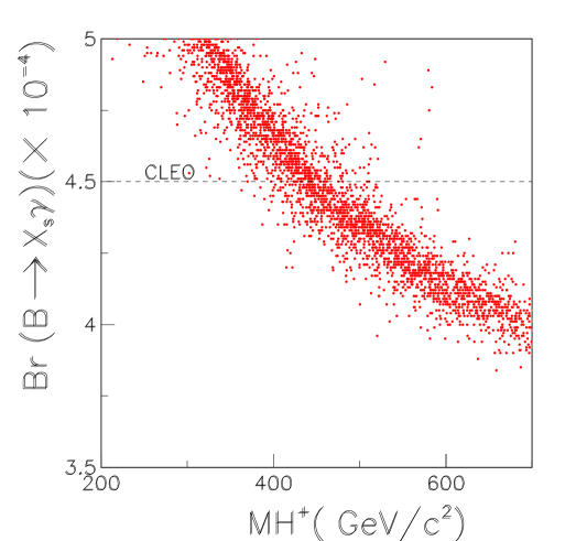
Figure 4: Branching ratio $B(b\to s\gamma)$ as a function of the charged Higgs boson mass $m_{H^{\pm}}$ in the limit of very heavy squark masses in MSSM–BRpV. The charged Higgs boson is defined as the massive charged scalar field with largest couplings to quarks.

In Fig. 4 we plot $B(b\to s\gamma)$ as a function of $m_{H^{\pm}}$ in the MSSM–BRpV model in the heavy squark limit. The difference is exclusively due to the mixing of the charged Higgs boson with the staus. The bound on the charged Higgs mass is in this case approximately $m_{H^{\pm}}>340$ GeV. Therefore, the bound is relaxed by about 100 GeV. The reason for the relaxation of the bound is simple. While the charged Higgs couplings to quarks diminish due to Higgs–Stau mixing, the contribution from the staus does not always compensate it, because staus may be heavier than the charged Higgs boson. It is important to stress that in Fig. 4 we have defined the charged Higgs as the field $S^{\pm}_{i}$ (excluding the massless Goldstone boson) that couples stronger to quarks, i.e., the massive field which maximizes the quantity $({\bf R}_{S^{\pm}}^{i1})^{2}+({\bf R}_{S^{\pm}}^{i2})^{2}$. Since in the charged Higgs loops contributing to $b\to s\gamma$ the relevant couplings are precisely those, this definition seems to be the most relevant for our purpose. Nevertheless, in order to compare, we have adopted a second way to decide which of the charged scalars we define as the charged Higgs.

In Fig. 5 we plot lower limits of $B(b\to s\gamma)$ as a function of $m_{H^{\pm}}$ in the MSSM–BRpV in the heavy squark limit. In the solid line we have the MSSM limit inferred from Fig. 3 and the dotted line is the MSSM–BRpV limit deduced from Fig. 4, where the charged Higgs is defined as the massive scalar with largest couplings to quarks. An alternative definition is to consider the charged Higgs boson as the massive field $S_{i}^{\pm}$ with largest component along $H^{\prime\pm}_{1}$ and $H^{\prime\pm}_{2}$, i.e., maximum $({\bf R^{\prime}}_{S^{\pm}}^{i1})^{2}+({\bf R^{\prime}}_{S^{\pm}}^{i2})^{2}$, as already explained in the text. This definition is motivated by the fact that in the rotated basis, where the epsilon term disappears from the superpotential, the rotated charged Higgs fields $H^{\prime\pm}_{1}$ and $H^{\prime\pm}_{2}$ decouple from the rotated staus fields as $v^{\prime}_{3}\to 0$. The corresponding lower limit of $B(b\to s\gamma)$ is represented by the dashed line in Fig. 5 and lies between the other two limits. We observe that the effect of the relaxation of the bound on $m_{H^{\pm}}$ is maintained although slightly weaker. The bound from the dashed line in Fig. 5 is approximately $m_{H^{\pm}}>370$ GeV, implying that BRpV relaxes the bound by about 70 GeV with respect to the MSSM.

Another interesting region of parameter space to explore is the region of light charged Higgs boson and light chargino. It is known that in order to have a light charged Higgs boson, its large contribution to $B(b\to s\gamma)$ must be canceled by the contribution from light charginos and stops. In Fig. 6 we plot the charged Higgs mass $m_{H^{\pm}}$ as a function of the lightest chargino mass $m_{\chi^{\pm}_{1}}$ within the MSSM. All the points satisfy the CLEO bound mentioned before. The solid vertical line is defined by $m_{\chi^{\pm}_{1}}=90$ GeV, which is approximately the experimental lower limit found by LEP2, at least for the heavy sneutrino case. Therefore, we can say that in order to have $m_{\chi^{\pm}_{1}}>90$ GeV, the CLEO measurement of $B(b\to s\gamma)$ implies that $m_{H^{\pm}}\>\raisebox{-2.15277pt}{$\stackrel{{\scriptstyle\textstyle>}}{{\sim}}$}\>110$ GeV in the MSSM.

As before, this bound on the charged Higgs boson mass is relaxed in the MSSM–BRpV model. In Fig. 7 we plot $m_{H^{\pm}}$ versus $m_{\chi^{\pm}_{1}}$ for points satisfying the CLEO bound on $B(b\to s\gamma)$ within the MSSM–BRpV. The charged Higgs boson is defined as the massive charged scalar with strongest couplings to quarks. We see from Fig. 7 that in order to have $m_{\chi^{\pm}_{1}}>90$ GeV compatible with $B(b\to s\gamma)$ we need $m_{H^{\pm}}\>\raisebox{-2.15277pt}{$\stackrel{{\scriptstyle\textstyle>}}{{\sim}}$}\>75$ GeV, therefore, relaxing the bound by about 35 GeV with respect to the MSSM.

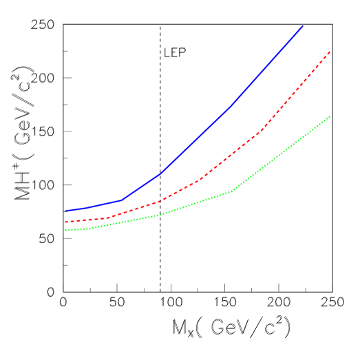
Figure 8: Lower limit of the charged Higgs boson mass as a function of the lightest chargino mass for $B(b\to s\gamma)$ compatible with CLEO measurement in the MSSM (solid) and in MSSM–BRpV (dashes and dots as explained in the text). The vertical dashed line corresponds to $m_{\chi_{1}}=90$ GeV.

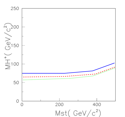
Figure 9: Lower limit of the charged Higgs boson mass as a function of the lightest stop mass for $B(b\to s\gamma)$ compatible with CLEO measurement in the MSSM (solid) and in the MSSM–BRpV (dashes and dots as explained in the text).

In Fig. 8 we give the lower bounds on $m_{H^{\pm}}$ as a function of the lightest chargino mass $m_{\chi^{\pm}_{1}}$. The solid curve corresponds to the MSSM limit extracted from Fig. 6 and the dotted curve corresponds to the MSSM–BRpV limit extracted from Fig. 7. If we define the charged Higgs boson as the massive field $S_{i}^{\pm}$ with largest component along the rotated charged Higgs fields $H^{\prime\pm}_{1}$ and $H^{\prime\pm}_{2}$, which decouple from the rotated staus fields as $v^{\prime}_{3}\to 0$, then we find the limit represented by the dashed curve. We see from this last curve that in order to have $m_{\chi^{\pm}_{1}}>90$ GeV compatible with $B(b\to s\gamma)$ we need $m_{H^{\pm}}\>\raisebox{-2.15277pt}{$\stackrel{{\scriptstyle\textstyle>}}{{\sim}}$}\>85$ GeV, therefore, relaxing the MSSM bound by about 25 GeV. In the same way, in Fig. 9 we plot the same lower bounds on $m_{H^{\pm}}$ but this time as a function of the lightest stop mass $m_{\tilde{t}_{1}}$. We observe from this figure that in order to cancel large contributions to $B(b\to s\gamma)$ due to a light charged Higgs boson, it is more important to have a light chargino rather than a light stop.

Now a word about the theoretical uncertainties on the calculation of $B(b\to s\gamma)$. If we assume a $10\%$ error, then the bound on the charged Higgs boson mass in the heavy stop limit within the MSSM reduces to $m_{H^{\pm}}\>\raisebox{-2.15277pt}{$\stackrel{{\scriptstyle\textstyle>}}{{\sim}}$}\>320$ GeV. For the same reason, the corresponding bounds on the MSSM–BRpV reduce to $m_{H^{\pm}}\>\raisebox{-2.15277pt}{$\stackrel{{\scriptstyle\textstyle>}}{{\sim}}$}\>200-250$ GeV, which corresponds to a decrease in 70–120 GeV, i.e., comparable to the values quoted above. No changes are observed in the case of light charged Higgs limits.

In summary, we have proved that the bounds on the charged Higgs mass of the MSSM coming from the experimental measurement of the branching ratio $B(b\to s\gamma)$ are relaxed if we add a single bilinear R–Parity violating term of the form $\epsilon_{3}\widehat{L}_{3}\widehat{H}_{2}$ to the superpotential. This term induces a tau neutrino mass which in models with universality of soft breaking mass parameters at the unification scale is naturally small. We study the effect of BRpV on $B(b\to s\gamma)$ by considering the unconstrained model where the values of all the unknown parameters are free at the weak scale. In this case the main constraint comes from the smallness of the tau neutrino mass. Even though in the MSSM–BRpV model the tau lepton mixes with charginos, implying that the tau-lepton also contributes to $B(b\to s\gamma)$ in loops with up–type squarks, we have shown that this contribution is negligible.

In contrast, in the MSSM–BRpV model the staus mix with the charged Higgs bosons and these contribute importantly to $B(b\to s\gamma)$ in loops with up–type quarks. For squark masses of a few TeV, where the chargino contribution is negligible, the charged Higgs mass in the MSSM has to satisfy $m_{H^{\pm}}\>\raisebox{-2.15277pt}{$\stackrel{{\scriptstyle\textstyle>}}{{\sim}}$}\>440$ GeV. This bound in the MSSM–BRpV turns out to be $m_{H^{\pm}}\>\raisebox{-2.15277pt}{$\stackrel{{\scriptstyle\textstyle>}}{{\sim}}$}\>340-370$ GeV, therefore, relaxing it in about 70–100 GeV. In order to have a light charged Higgs boson in SUSY, its large contribution to $B(b\to s\gamma)$ can only be compensated by a large contribution from a light chargino and squark. In order to satisfy the experimental bound on $B(b\to s\gamma)$ with $m_{\chi^{\pm}_{1}}>90$ GeV in the MSSM it is necessary to have $m_{H^{\pm}}\>\raisebox{-2.15277pt}{$\stackrel{{\scriptstyle\textstyle>}}{{\sim}}$}\>110$ GeV. In the MSSM–BRpV model this bound is $m_{H^{\pm}}\>\raisebox{-2.15277pt}{$\stackrel{{\scriptstyle\textstyle>}}{{\sim}}$}\>75-85$ GeV, i.e. 25–35 GeV weaker than in the MSSM. It is important to note that, in contrast to the MSSM, charged Higgs boson masses as small as these can be achieved in MSSM–BRpV already at tree level, as discussed in ref. [23]. The reason to the relaxation of the MSSM bounds can be understood as follows: while the charged Higgs couplings to quarks diminish with the presence of Higgs–Stau mixing, the contribution from the staus not always compensate this decrease because the stau mass is, in general, different from the charged Higgs boson mass, and could be larger.

Finally, a last word on our results on Fig. 5, 8 and 9 represented by the dashed and dotted curves. These denote the Higgs mass bounds we have obtained in the MSSM-BRpV model, when different basis are chosen to perform the calculation. The point to stress is that our results do not depend on the choice of basis as such. They depend only on our criterium for specifying which state corresponds to the Higgs boson and it is here where we have suggested two possible definitions which are motivated by two possible basis choices.

Figure 1: Chargino/tau amplitude contributing to $B(b\to s\gamma)$ as a function of the squark soft mass parameter $M_{Q}$ in MSSM–BRpV.

Figure 2: Tau amplitude contributing to $B(b\to s\gamma)$ as a function of the squark soft mass parameter $M_{Q}$ in MSSM–BRpV.

Figure 3: Branching ratio $B(b\to s\gamma)$ as a function of the charged Higgs boson mass $m_{H^{\pm}}$ in the limit of very heavy squark masses within the MSSM.

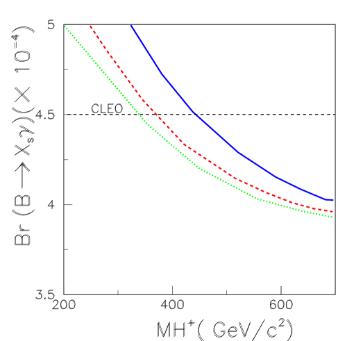
Figure 5: Lower limit on the branching ratio $B(b\to s\gamma)$ as a function of the charged Higgs boson mass $m_{H^{\pm}}$. We consider the limit of very heavy squark masses within the MSSM (solid) and the MSSM–BRpV (dashes and dots as explained in the text).

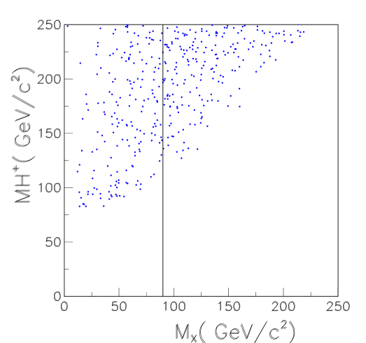
Figure 6: Charged Higgs boson mass as a function of the lightest chargino mass for $B(b\to s\gamma)$ compatible with CLEO measurement within the MSSM. The vertical dashed line corresponds to $m_{\chi_{1}}=90$ GeV.

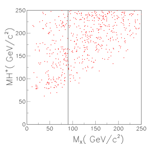
Figure 7: Charged Higgs boson mass as a function of the lightest chargino mass for $B(b\to s\gamma)$ compatible with CLEO measurement in MSSM–BRpV. The charged Higgs is defined as the massive charged scalar field with largest couplings to quarks. The vertical dashed line corresponds to $m_{\chi_{1}}=90$ GeV.

References

[1]
CLEO Collaboration (M.S. Alam et al.), Phys. Rev. Lett.74,
2885 (1995).
[2]
CLEO Collaboration (S. Glenn et al.), CLEO CONF 98-17. Talk presented at the
XXIX Intl. Conf. on High Energy Physics, ICHEP98. UBC, Vancouver, B.C., Canada, July 23-29 1998.
[3]
ALEPH Collaboration (R. Barate et al.), Report No. CERN–EP/98–044,
March 1998. Submitted to Phys. Lett. B.
[4]
K. Chetyrkin, M. Misiak, and M. Münz, Phys. Lett. B400,
206 (1997).
[5]
J.L. Hewett, Phys. Rev. Lett.70, 1045 (1993);
V. Barger, M.S. Berger, and R.J.N. Phillips, Phys. Rev. Lett.70, 1368 (1993).
[7]
S. Bertolini, F. Borzumati, A. Masiero, and G. Ridolfi,
Nucl. Phys.B353, 591 (1991).
[8]
M.A. Díaz, Phys. Lett. B304, 278 (1993).
[9]
R. Barbieri and G.F. Giudice, Phys. Lett. B309, 86 (1993).
[10]
N. Oshimo, Nucl. Phys.B404, 20 (1993);
J.L. Lopez, D.V. Nanopoulos, and G.T. Park, Phys. Rev. D48,
974 (1993);
Y. Okada, Phys. Lett. B315, 119 (1993);
R. Garisto and J.N. Ng, Phys. Lett. B315, 372 (1993);
J.L. Lopez, D.V. Nanopoulos, G.T. Park, and A. Zichichi,
Phys. Rev. D49, 355 (1994);
M.A. Díaz, Phys. Lett. B322, 207 (1994);
F.M. Borzumati, Z. Phys.C63, 291 (1994);
S. Bertolini and F. Vissani, Z. Phys.C67, 513 (1995);
J. Wu, R. Arnowitt, and P. Nath, Phys. Rev. D51, 1371 (1995);
T. Goto and Y. Okada, Prog. Theo. Phys.94, 407 (1995);
B. de Carlos and J.A. Casas, Phys. Lett. B349, 300 (1995),
erratum-ibid. B351 604 (1995).
[11]
G.V. Kraniotis, Z. Phys. C71, 163 (1996);
T.V. Duong, B. Dutta, and E. Keith, Phys. Lett. B378,
128 (1996);
G.T. Park, Mod. Phys. Lett.A11, 1877 (1996);
C.-H. Chang and C. Lu, Commun. Theor. Phys.27, 331 (1997);
H. Baer and M. Brhlik, Phys. Rev. D55, 3201 (1997);
N.G. Deshpande, B. Dutta and S. Oh, Phys. Rev. D56, 519 (1997);
R. Martinez and J-A. Rodriguez, Phys. Rev. D55, 3212 (1997);
S. Khalil, A. Masiero, and Q. Shafi, Phys. Rev. D56, 5754
(1997).
[12]
S. Bertolini and J. Matias, hep-ph/9709330;
T. Blazek and S. Raby, hep-ph/9712257;
H. Baer, M. Brhlik, D. Castano, and X. Tata, hep-ph/9712305;
W. de Boer, H.-J. Grimm, A.V. Gladyshev, and D.I. Kazakov, hep-ph/9805378.
[13]
C. Greub, T. Hurth, and D. Wyler, Phys. Lett. B380, 385 (1996);
Phys. Rev. D54, 3350 (1996).
[14]
K. Adel and Y.P. Yao, Phys. Rev. D49, 4945 (1994).
[15]
M. Ciuchini, G. Degrassi, P. Gambino, and G.F. Giudice, Report No.
CERN–TH/97–279, Oct 1997, hep–ph/9710335.
[16]
A. Ali and C. Greub Zeit. für Physik C49, 431 (1991);
Phys. lett. B259, 182 (1991); Phys. lett. B361,
146 (1995); N. Pott, Phys. Rev. D54, 938 (1996).
[17]
K. Chetyrkin, M. Misiak, and M. Münz, Report No. MPI-PHT-97-45,
Nov 1997, hep–ph/9711266.
[18]
A.J. Buras, M. Jamin, M.E. Lautenbacher, and P.H. Weisz, Nucl.
Phys. B370, 69 (1992); M. Misiak and M. Münz, Phys.
Lett. B344, 308 (1995).
[19]
A. Masiero and J.W.F. Valle, Phys. Lett. B251, 273 (1990);
J.C. Romão, A. Ioannissyan and J.W.F. Valle,
Phys. Rev. D55, 427 (1997).
[20]
M.C. González-García, J. W. F. Valle Nucl.Phys.B355:330-350,1991; K. Huitu, J. Maalampi, K. Puolamaki, e-Print
Archive: hep-ph/9705406
[21]
F. de Campos, M.A. García-Jareño, A.S. Joshipura, J. Rosiek,
and J.W.F. Valle, Nucl. Phys.B451, 3 (1995);
A. S. Joshipura and M.Nowakowski, Phys. Rev.D51, 2421 (1995);
T. Banks, Y. Grossman, E. Nardi, and Y. Nir, Phys. Rev. D52, 5319 (1995);
R. Hempfling, Nucl. Phys.B478, 3 (1996);
F. Vissani and A.Yu. Smirnov, Nucl.Phys.B460, 37 (1996);
H. P. Nilles and N. Polonsky, Nucl. Phys.B484, 33 (1997);
B. de Carlos, P. L. White, Phys.Rev.D55, 4222 (1997);
S. Roy and B. Mukhopadhyaya, Phys. Rev. D55, 7020 (1997);
M. Bisset, O.C.W. Kong, C. Macesanu, and L.H. Orr, hep-ph/9804282.
[22]
M.A. Díaz, J.C. Romão, and J.W.F. Valle, Nucl. Phys. B 524 (1998) 23-40
[hep-ph/9706315].
[23]
A. Akeroyd, M.A. Díaz, J. Ferrandis, M.A. Garcia–Jareño,
and J.W.F. Valle, hep-ph/9707395, Nucl. Phys. B xxx (1998) xx in press
[24]
M.A. Díaz, J. Ferrandis, J.C. Romão, and J.W.F. Valle,
hep-ph/9801391; A. Akeroyd, M.A. Díaz, and J.W.F. Valle,
hep-ph/9806382.
[25]
M. Bisset, O.C.W. Kong, C. Macesanu, and L.H. Orr, hep-ph/9804282.
[27]
Jose W. F. Valle, Invited talk at the Workshop on Physics beyond the
Standard Model Accelerator- and Non-Accelerator approaches (”Beyond
the Desert”) Germany, June 1997, hep-ph/9712277.
[28]
F. de Campos, O. J. P. Eboli, M. A. Garcia-Jareno, J. W. F. Valle,
hep-ph/9710545, Nucl. Phys. B.
[29] M. Misiak, S. Pokorski, and J. Rosiek, hep-ph/9703442.