Dipole Form Factors and Loop–induced
CP violation in Supersymmetry

Abstract

The one–loop Minimal Supersymmetric Standard Model (MSSM) contributions to the weak and electromagnetic dipole form factors of heavy fermions are reviewed. For the $Z$ boson on shell, the weak–magnetic and weak–electric dipole moments of the $\tau$ lepton and the $b$ quark can be defined and directly connected to observables. But far from the $Z$ peak, the weak and electromagnetic dipole form factors are not enough to account for all the new physics effects. In the context of the calculation of the process $e^{+}e^{-}\to t\bar{t}$ to one loop in the MSSM, we compare the impact on the phenomenology of the CP–violating dipole form factors of the top quark with the contribution from CP–violating box graphs. Some exemplificative observables are analyzed and the relevance of both the contributions is pointed out. The set of tensor integrals employed, the one–loop expressions for the electromagnetic and weak dipole form factors in a general renormalizable theory and the SM and MSSM couplings and conventions are also given.

1 Introduction

The investigation of the electric and magnetic dipole moments of fermions provides deep insight in particle theory. The measurement of the intrinsic magnetic dipole moment (MDM) of the electron proved the correctness of the hypothesis of half–integer spin particles [1] and is one of the most spectacular achievements of quantum field theory predictions. More precise studies of electron and muon showed afterwards the presence of an anomalous contribution to the MDM (AMDM) and imply very accurate tests of the quantum structure of the Standard Model (SM). The measurements of the $(g_{e}-2)$ and $(g_{\mu}-2)$ available [2] are in perfect agreement with the SM predictions to several orders in the perturbative expansion of the theory (cf. [3] and references therein). Furthermore, with the expected precision at the E821 Brookhaven experiment [4] it will be possible to improve the previous measurement of $(g_{\mu}-2)$ by a factor 20. Therefore the MDMs can be used, together with the precision tests at the $Z$ resonance from LEP and SLC and the new results of LEP2 and TEVATRON, to set bounds on possible New Physics effects beyond the SM [5].

The importance of the analysis of the electric dipole moment (EDM) of elementary and composite particles is intimately related to the CP violating character of the theory. In the electroweak SM there is only one possible source of CP violation, the $\delta_{\rm CKM}$ phase of the Cabibbo–Kobayashi–Maskawa (CKM) mixing matrix for quarks [6]. Currently the only place where CP violation has been measured, the neutral $K$ system, fixes the value of this phase but does not constitute itself a test for the origin of CP violation [7]. On the other hand, if the baryon asymmetry of the universe has been dynamically generated, CP must be violated. The SM cannot account for the size of the observed asymmetry [8]. In extended models (beyond the SM) many other possible explanations of CP violation can be given. In particular, in supersymmetric (SUSY) models [9, 10] CP violation can appear assuming complex soft–SUSY–breaking terms. Two physical phases remain in the GUT constrained MSSM [10, 11, 12], enough to provide the correct size of baryon asymmetry in some range of parameters [13]. But the most significant effect of the CP violating phases in the phenomenology is their contribution to the EDMs [14]. Unlike the SM, where the contribution to the EDM of fermions arises beyond two loops [15], the MSSM can give a contribution already at the one–loop level [9].

The measurements of the neutron, electron and muon EDMs [16, 17] constrain the phases and the supersymmetric spectrum in a way that may demand fine tuning (supersymmetric CP problem): SUSY particles very heavy (several TeV [18]) or phases of ${\cal O}(10^{-2})$ [9]. Very large soft–SUSY–breaking masses are unappealing as it seems natural to demand the SUSY spectrum to be at the electroweak scale. On the other side, general universal soft–SUSY–breaking terms can be taken only if the genuine SUSY CP phases are vanishing. In this case the CP violation is originated via the usual SM CKM mechanism and the supersymmetric spectrum affects the observables only through renormalization group equations and/or one–loop radiative contributions. Of course in this scenario one has to construct models in which the SUSY phases naturally vanish [19] and at the same time provide some other non–standard mechanism for explaining electroweak baryogenesis. There exist also ways of naturally obtaining small non–zero soft–phases which leave sufficient CP violation for baryogenesis [12]. But, in general, to get observable effects in most electroweak processes one has to relax the assumption of soft–term universality. Several attempts have been made, following this direction, to use CP violation from top–squark mixing: a complex parameter $A_{t}$ would yield large CP violating effects in collider processes involving top quarks [20]. Besides, due to renormalization–group–induced effects on the other low energy phases, the phase of $A_{t}$ is constrained by the EDM of the neutron [22]. One can also make the hypothesis that, due to cancellation among the different components of the neutron EDM (constituent quarks and gluons), the SUSY phases can still be kept of ${\cal O}(1)$ and the SUSY spectrum at the electroweak scale satisfying the experimental bounds [23]. Finally, in [24] it is shown that, in the constrained MSSM, large CP violating phases are compatible with the bounds on the electron and neutron EDMs as well as with the cosmological relic densities. In view of all these arguments we keep our analysis completely general and consider the SUSY CP–phases as free parameters.

Some attention has also been payed to the study of possible CP violating effects in the context of R–parity violating models [25]. In this class of models new interactions appear providing extra sources of CP violation (still preventing fast proton decay). They can explain the CP violation in the $K$ system (with no need of the CKM phase) without introducing anomalous Flavor Changing Neutral Current (FCNC) contributions [26]. In any case we assume in the following R–parity conservation for simplicity.

Recently a number of works have been devoted to the analysis of weak dipole moments (WDM). The WDMs are defined, in analogy to the usual DMs, taking the corresponding on–shell chirality–flipping form factors of the $Zff$ effective vertex. The SM one–loop contribution to the anomalous weak magnetic dipole moment (AWMDM) has been calculated for the $\tau$ lepton and the $b$ quark in [27, 28]. The CP–violating weak electric dipole moment (WEDM) is in the SM a tiny three–loop effect. The WDMs are gauge invariant and can directly connected to physical observables. While for the $\tau$ case, using appropriate observables [27, 29, 30], an experimental analysis is feasible, for the $b$ case the situation is complicated by hadronization effects [31]. The SM predictions are far below the sensitivity reachable at LEP [27] but non–standard interactions can enhance these expectations (2HDM [32], MSSM [33]) especially for the (CP–violating) WEDMs (2HDM, leptoquark models [34], MSSM [35]). The experimental detection of non–zero AWMDM or WEDM of heavy fermions, at the current sensitivity, would be a clear evidence of new physics beyond the SM.

In the perspective of the next generation of linear $e^{+}e^{-}$ colliders, we extend the previous analyses on the WDMs to consider the $t$ quark dipole form factors (DFF) and, in particular, the CP–violating ones. In [36] an independent analysis of the $t$ quark EDFF and WEDFF can be found. Since the $t$ quark is very heavy one expects this fermion to be the best candidate to have larger DFFs. Beyond the $Z$ peak ($s>4m^{2}_{t}$) other effects are expected to give contributions to the physical observables. In fact the DFFs in a general model are not guaranteed to be gauge independent. An exception is the one–loop MSSM contribution to the CP–violating electromagnetic and weak DFFs (EDFF and WEDFF) which do not involve any gauge boson in internal lines. Anyway, although this contribution is indeed gauge invariant any CP–odd observable will be sensitive to not only the DFFs but to the complete set of one–loop CP–violating diagrams involved. In this work we present the full calculation of the expectation value of a set of these observables in the context of the MSSM and compare the size of the different contributions.

The paper is organized as follows. In Section 2 we present the general effective vertex describing the interaction of on–shell fermions with a neutral vector boson. The definitions and the generic expressions of the DFFs for all the contributing topologies at the one–loop level are also given. In Section 3 we evaluate these expressions for on–shell $Z$ and the case of the $\tau$ lepton and the $b$ quark (their AWMDM and WEDM) in the context of the SM and the MSSM. A discussion of the supersymmetric limit is also given. The evaluation of the $t$ quark EDFFs and WEDFFs at $\sqrt{s}=500$ GeV is presented in Section 4. In Section 5 we review observables sensitive to the $\tau$ AWMDM at the $Z$ peak as well as other CP–odd observables valid in general. In Section 6 we evaluate specific CP–odd observables for the $t$ quark pair production in $e^{+}e^{-}$ colliders to one loop in the MSSM and compare the influence of the $t$ EDFF and WEDFF with that of the CP–violating box diagrams. Our conclusions are presented in Section 7. In the Appendices one can find the definition of the one–loop tensor integrals and the SM and MSSM couplings and conventions that have been used.

2 The dipole form factors

2.1 The $Vff$ effective vertex

The most general effective Lagrangian describing the interaction of a neutral vector boson $V$ with two fermions can be written, using at most dimension five operators, as a function of ten independent terms:

$${\cal L}_{Vff} = V^{\mu}(x)\bar{\Psi}(x)\Bigg{[}\gamma_{\mu}\left(g_{\rm V}-g_{\rm A}\gamma_{5}\right)\ +\ {\rm i}\stackrel{{\scriptstyle\leftrightarrow}}{{\partial_{\mu}}}\left(g_{\rm M}+{\rm i}g_{\rm E}\gamma_{5}\right)$$ (1)

$$\qquad\qquad\qquad+{\rm i}\stackrel{{\scriptstyle\leftrightarrow}}{{\partial^{\nu}}}\sigma_{\mu\nu}\left(g_{\rm TS}+{\rm i}g_{\rm TP}\gamma_{5}\right)\Bigg{]}\Psi(x)\$$

$$+ \left({\rm i}\partial^{\mu}V^{\nu}(x)\right)\bar{\Psi}(x)\Bigg{[}g_{\mu\nu}\left({\rm i}g_{\rm S}+g_{\rm P}\gamma_{5}\right)\ +\ \sigma_{\mu\nu}\left({\rm i}g_{\rm TM}+g_{\rm TE}\gamma_{5}\right)\Bigg{]}\Psi(x).$$

The first two coefficients, i.e. $g_{\rm V}$ and $g_{\rm A}$, are the usual vector and axial–vector couplings. They are connected to chirality conserving dimension four operators. All the other coefficients in Eq. (1) multiply chirality flipping dimension five operators and can receive a contribution only through radiative corrections in a renormalizable theory. The operators associated to $g_{\rm V}$, $g_{\rm A}$, $g_{\rm M}$, $g_{\rm P}$, $g_{\rm TM}$ and $g_{\rm TP}$ are even under a CP transformation. The presence of non vanishing $g_{\rm E}$, $g_{\rm S}$, $g_{\rm TE}$ and $g_{\rm TS}$ yields a contribution to CP–violating observables. In Table 1 we summarize the C, P, T and chirality properties of each operator introduced in the effective Lagrangian.

Table 1: C, P, T properties of the operators in the effective Lagrangian of Eq. (1). Their chirality flipping behavior is also displayed.

Operator	Coefficient	P	CP	T	Chirality Flip
$V^{\mu}\bar{\Psi}\gamma_{\mu}\Psi$	$g_{\rm V}$	$+$	$+$	$+$	NO
$V^{\mu}\bar{\Psi}\gamma_{\mu}\gamma_{5}\Psi$	$g_{\rm A}$	$-$	$+$	$+$	NO
$V^{\mu}\bar{\Psi}{\rm i}\stackrel{{\scriptstyle\leftrightarrow}}{{\partial_{\mu}}}\Psi$	$g_{\rm M}$	$+$	$+$	$+$	YES
$V^{\mu}\bar{\Psi}\stackrel{{\scriptstyle\leftrightarrow}}{{\partial_{\mu}}}\gamma_{5}\Psi$	$g_{\rm E}$	$-$	$-$	$-$	YES
$V^{\mu}\bar{\Psi}{\rm i}\stackrel{{\scriptstyle\leftrightarrow}}{{\partial^{\nu}}}\sigma_{\mu\nu}\Psi$	$g_{\rm TS}$	$+$	$-$	$-$	YES
$V^{\mu}\bar{\Psi}\stackrel{{\scriptstyle\leftrightarrow}}{{\partial^{\nu}}}\sigma_{\mu\nu}\gamma_{5}\Psi$	$g_{\rm TP}$	$-$	$+$	$+$	YES
$\left(\partial\cdot V\right)\bar{\Psi}\Psi$	$g_{\rm S}$	$+$	$-$	$-$	YES
$\left({\rm i}\partial\cdot V\right)\bar{\Psi}\gamma_{5}\Psi$	$g_{\rm P}$	$-$	$+$	$+$	YES
$\left(\partial^{\mu}V^{\nu}\right)\bar{\Psi}\sigma_{\mu\nu}\Psi$	$g_{\rm TM}$	$+$	$+$	$+$	YES
$\left({\rm i}\partial^{\mu}V^{\nu}\right)\bar{\Psi}\sigma_{\mu\nu}\gamma_{5}\Psi$	$g_{\rm TE}$	$-$	$-$	$-$	YES

By Fourier transform of Eq. (1) one obtains the most general Lorentz structure for the vertex $Vff$ in the momentum space:

$$\Gamma^{Vff}_{\mu} = {\rm i}\Bigg{[}\gamma_{\mu}\left(f_{\rm V}-f_{\rm A}\gamma_{5}\right)\ +\ (q-\bar{q})_{\mu}\left(f_{\rm M}+{\rm i}f_{\rm E}\gamma_{5}\right)+\ p_{\mu}\left({\rm i}f_{\rm S}+f_{\rm P}\gamma_{5}\right)$$ (2)

$$\qquad+(q-\bar{q})^{\nu}\sigma_{\mu\nu}\left(f_{\rm TS}+{\rm i}f_{\rm TP}\gamma_{5}\right)\ +\ p^{\nu}\sigma_{\mu\nu}\left({\rm i}f_{\rm TM}+f_{\rm TE}\gamma_{5}\right)\Bigg{]},$$

where $q$ and $\bar{q}$ are the outgoing momenta of the fermions and $p=(q+\bar{q})$ is the total incoming momentum of the neutral boson $V$. The form factors $f_{i}$ are functions of the kinematical invariants. Actually they are more general than the coefficients $g_{i}$. In fact any operator of dimension higher than five added to the Lagrangian of Eq. (1) is related to a new coefficient $g_{i}$. But every new coefficient can contribute only to the ten independent form factors $f_{i}$ introduced in Eq. (2). The parameters $g_{i}$ and the form factors $f_{i}$ can be complex in general. Their real parts account for dispersive effects (CPT–even) whereas their imaginary parts are related to absorptive contributions.

It is possible to lower the number of independent form factors in Eq. (2) by imposing on–shell conditions on the fermionic and/or bosonic fields. For instance, in the case of on–shell fermions, making use of the Gordon identities:

$$2m_{f}~{}\bar{u}~{}\gamma^{\mu}~{}v = \Big{\{}\bar{u}~{}(q-\bar{q})^{\mu}~{}v+\bar{u}~{}{\rm i}~{}(q+\bar{q})_{\nu}\sigma^{\mu\nu}~{}v\Big{\}},$$

$$2m_{f}~{}\bar{u}~{}\gamma^{\mu}\gamma_{5}~{}v = \Big{\{}\bar{u}~{}(q+\bar{q})^{\mu}\gamma_{5}~{}v+\bar{u}~{}{\rm i}~{}(q-\bar{q})_{\nu}\sigma^{\mu\nu}\gamma_{5}~{}v\Big{\}},$$

$$0 = \Big{\{}\bar{u}~{}(q+\bar{q})^{\mu}~{}v+\bar{u}~{}{\rm i}~{}(q-\bar{q})_{\nu}\sigma^{\mu\nu}v\Big{\}},$$

$$0 = \Big{\{}\bar{u}~{}(q-\bar{q})^{\mu}~{}\gamma_{5}~{}v+\bar{u}~{}{\rm i}~{}(q+\bar{q})_{\nu}\sigma^{\mu\nu}\gamma_{5}~{}v\Big{\}}~{},$$ (3)

one can eliminate $f_{\rm TM}$, $f_{\rm TE}$, $f_{\rm TS}$ and $f_{\rm TP}$ from the effective Lagrangian. The number of relevant form factors can be further reduced taking also the boson $V$ on its mass shell. In this case the condition $p_{\mu}\epsilon^{\mu}=0$ automatically cancels all the contributions coming from $f_{\rm S}$ and $f_{\rm P}$. The same situation occurs for off–shell vector boson $V$ when, in the process $e^{+}e^{-}\to V^{*}\to f\bar{f}$, the electron mass is neglected. Therefore $f_{\rm S}$ and $f_{\rm P}$ will be ignored in the following. With all these assumptions the $Vff$ effective vertex for on–shell fermions is conventionally written as:

$$\Gamma^{Vff}_{\mu}(s)={\rm i}e\Bigg{\{}\gamma_{\mu}\left[V^{V}_{f}(s)-A^{V}_{f}(s)\gamma_{5}\right]+\sigma_{\mu\nu}(q+\bar{q})^{\nu}\Bigg{[}{\rm i}\frac{a^{V}_{f}(s)}{2m_{f}}-\frac{d^{V}_{f}(s)}{e}\gamma_{5}\Bigg{]}\Bigg{\}},$$ (4)

where $e$ and $m_{f}$ are respectively the electric unit charge and the mass of the external fermion. The form factors in Eq. (4) depend only on $s$. As mentioned above $V^{V}_{f}(s)$ and $A^{V}_{f}(s)$ parameterize the vector and axial–vector current. They are connected to the chirality conserving CP–even sector. The form factors $a^{V}_{f}(s)$ and $d^{V}_{f}(s)$ are known respectively as anomalous magnetic dipole form factor (AMDFF) and electric dipole form factor (EDFF). They are both connected to chirality flipping operators. In a renormalizable theory they can receive contribution exclusively by quantum corrections. The EDFFs contribute to the CP–odd sector and constitute a source of CP–violation.

The dipole moments (DM) are defined taking the corresponding vector bosons on shell, $s=M^{2}_{V}$. For $V=\gamma$ one gets the usual definitions of the photon anomalous magnetic dipole moment (AMDM) and electric dipole moment (EDM). The definitions of electric charge, magnetic and electric dipole moments [37] consistent with our convention for the covariant derivative (131) are respectively:

charge $$\equiv -e\ V^{\gamma}_{f}(0)=e\ Q_{f}\ ,$$ (5)

MDM $$\equiv \frac{e}{2m_{f}}(V^{\gamma}_{f}(0)+a^{\gamma}_{f}(0))\ ,$$ (6)

EDM $$\equiv d^{\gamma}_{f}(0)\ .$$ (7)

Thus the AMDM of a fermion is $a^{\gamma}_{f}(0)=-Q_{f}(g_{f}-2)/2$ with $g_{f}$ being the gyromagnetic ratio. The axial-vector coupling $A^{\gamma}_{f}$ vanishes. For $V=Z$, the quantities $a^{w}_{f}\equiv a^{Z}_{f}(M^{2}_{Z})$ and $d^{w}_{f}\equiv d^{Z}_{f}(M^{2}_{Z})$ define the anomalous weak–magnetic dipole moment (AWMDM) and the weak–electric dipole moment (WEDM).

2.2 One–loop generic expressions of the dipole form factors

All the possible one–loop contributions to the $a^{V}_{f}(s)$ and $d^{V}_{f}(s)$ form factors can be classified in terms of the six classes of triangle diagrams depicted in Fig. 1.

Figure 1: The one-loop $Vff$ diagrams with general couplings.

The vertices involved are labelled by generic couplings for vector bosons $V^{(k)}_{\mu}=A_{\mu},\ Z_{\mu},\ W_{\mu},\ W^{\dagger}_{\mu}$, fermions $\Psi_{k}$ and scalar bosons $\Phi_{k}$, according to the following interaction Lagrangian:

$${\cal L} = {\rm i}eJ(W^{\dagger}_{\mu\nu}W^{\mu}V^{\nu}-W^{\mu\nu}W^{\dagger}_{\mu}V_{\nu}+V^{\mu\nu}W^{\dagger}_{\mu}W_{\nu})+{\rm i}eG_{jk}V^{\mu}\Phi_{j}^{\dagger}\stackrel{{\scriptstyle\leftrightarrow}}{{\partial}}_{\mu}\Phi_{k}$$ (8)

$$+\Big{\{}e\bar{\Psi}_{f}(S_{jk}-P_{jk}\gamma_{5})\Psi_{k}\Phi_{j}\ +eK_{jk}V^{\mu}V^{(k)}_{\mu}\Phi_{j}+{\rm h.c.}\Big{\}}$$

$$+eV^{(k)}_{\mu}\bar{\Psi}_{j}\gamma^{\mu}(V^{(k)}_{jl}-A^{(k)}_{jl}\gamma_{5})\Psi_{l}\ .$$

Every class of diagrams is calculated analytically and expressed in terms of the couplings introduced in (8) and the one–loop three–point integrals $\bar{C}_{i}$ (see App. A). The result is given in the ’t Hooft-Feynman gauge.

• [Class I]: vector–boson exchange:

  $$\frac{a^{V}_{f}(s)}{2m_{f}}({\rm I}) = \frac{\alpha}{4\pi}\Big{\{}4m_{f}\sum_{jkl}{\rm Re}\Big{[}V^{(V)}_{jk}(V^{(l)}_{fj}V^{(l)*}_{fk}+A^{(l)}_{fj}A^{(l)*}_{fk})$$ (9)

  $$\hskip 56.9055pt+A^{(V)}_{jk}(V^{(l)}_{fj}A^{(l)*}_{fk}+A^{(l)}_{fj}V^{(l)*}_{fk})\Big{]}\Big{[}2C^{+}_{2}-3C^{+}_{1}+C_{0}\Big{]}_{kjl}$$

  $$\hskip 22.76228pt+4\sum_{jkl}m_{k}{\rm Re}\Big{[}V^{(V)}_{jk}(V^{(l)}_{fj}V^{(l)*}_{fk}-A^{(l)}_{fj}A^{(l)*}_{fk})$$

  $$\hskip 56.9055pt-A^{(V)}_{jk}(V^{(l)}_{fj}A^{(l)*}_{fk}-A^{(l)}_{fj}V^{(l)*}_{fk})\Big{]}\Big{[}2C^{+}_{1}-C_{0}\Big{]}_{kjl}\Big{\}}$$

  $$\frac{d^{V}_{f}(s)}{e}({\rm I}) = \frac{\alpha}{4\pi}\Big{\{}4m_{f}\sum_{jkl}{\rm Im}\Big{[}V^{(V)}_{jk}(V^{(l)}_{fj}A^{(l)*}_{fk}+A^{(l)}_{fj}V^{(l)*}_{fk})$$ (10)

  $$\hskip 56.9055pt+A^{(V)}_{jk}(V^{(l)}_{fj}V^{(l)*}_{fk}+A^{(l)}_{fj}A^{(l)*}_{fk})\Big{]}\Big{[}2C^{+-}_{2}-C^{-}_{1}\Big{]}_{kjl}$$

  $$\hskip 22.76228pt-4\sum_{jkl}m_{k}{\rm Im}\Big{[}V^{(V)}_{jk}(V^{(l)}_{fj}A^{(l)*}_{fk}-A^{(l)}_{fj}V^{(l)*}_{fk})$$

  $$\hskip 56.9055pt-A^{(V)}_{jk}(V^{(l)}_{fj}V^{(l)*}_{fk}-A^{(l)}_{fj}A^{(l)*}_{fk})\Big{]}\Big{[}2C^{+}_{1}-C_{0}\Big{]}_{kjl}\Big{\}}$$

  In the case of gluon exchange one has to substitute $\alpha$ for $\alpha_{s}$ and $V^{(l)}_{fi}$ for $T_{l}$ (the SU(3) generators) and take $A^{(l)}_{fj}=0$. The sum over the index $l$ yields a color factor $C_{F}=4/3$. The gluon contribution to the CP–violating form factor $d^{V}_{f}({\rm I}$) vanishes in general.

• [Class II]: fermion exchange and two internal vector bosons:

  $$\frac{a^{V}_{f}(s)}{2m_{f}}({\rm II}) = \frac{\alpha}{4\pi}\Big{\{}2m_{f}\sum_{jkl}{\rm Re}\Big{[}J(V^{(j)}_{fl}V^{(k)*}_{fl}+A^{(j)}_{fl}A^{(k)*}_{fl})\Big{]}\Big{[}4C^{+}_{2}+C^{+}_{1}\Big{]}_{kjl}$$ (11)

  $$\hskip 28.45274pt-6\sum_{jkl}m_{l}{\rm Re}\Big{[}J(V^{(j)}_{fl}V^{(k)*}_{fl}-A^{(j)}_{fl}A^{(k)*}_{fl})\Big{]}\Big{[}C^{+}_{1}\Big{]}_{kjl}\Big{\}}$$

  $$\frac{d^{V}_{f}(s)}{e}({\rm II}) = -\frac{\alpha}{4\pi}\Big{\{}2m_{f}\sum_{jkl}{\rm Im}\Big{[}J(V^{(j)}_{fl}A^{(k)*}_{fl}+A^{(j)}_{fl}V^{(k)*}_{fl})\Big{]}\Big{[}4C^{+-}_{2}-C^{-}_{1}\Big{]}_{kjl}$$ (12)

  $$\hskip 28.45274pt+6\sum_{jkl}m_{l}{\rm Im}\Big{[}J(V^{(j)}_{fl}A^{(k)*}_{fl}-A^{(j)}_{fl}V^{(k)*}_{fl})\Big{]}\Big{[}C^{+}_{1}\Big{]}_{kjl}\Big{\}}$$

• [Class III]: scalar exchange:

  $$\frac{a^{V}_{f}(s)}{2m_{f}}({\rm III}) = \frac{\alpha}{4\pi}\Big{\{}2m_{f}\sum_{jkl}{\rm Re}\Big{[}V^{(V)}_{jk}(S_{lj}S^{*}_{lk}+P_{lj}P^{*}_{lk})$$ (13)

  $$\hskip 56.9055pt+A^{(V)}_{jk}(S_{lj}P^{*}_{lk}+P_{lj}S^{*}_{lk})\Big{]}\Big{[}2C^{+}_{2}-C^{+}_{1}\Big{]}_{kjl}$$

  $$\hskip 22.76228pt-2\sum_{jkl}{m}_{k}{\rm Re}\Big{[}V^{(V)}_{jk}(S_{lj}S^{*}_{lk}-P_{lj}P^{*}_{lk})$$

  $$\hskip 56.9055pt-A^{(V)}_{jk}(S_{lj}P^{*}_{lk}-P_{lj}S^{*}_{lk})\Big{]}\Big{[}C^{+}_{1}+C^{-}_{1}\Big{]}_{kjl}\Big{\}}$$

  $$\frac{d^{V}_{f}(s)}{e}({\rm III}) = \frac{\alpha}{4\pi}\Big{\{}-2m_{f}\sum_{jkl}{\rm Im}\Big{[}V^{(V)}_{jk}(P_{lj}S^{*}_{lk}+S_{lj}P^{*}_{lk})$$ (14)

  $$\hskip 56.9055pt+A^{(V)}_{jk}(S_{lj}S^{*}_{lk}+P_{lj}P^{*}_{lk})\Big{]}\Big{[}2C^{+-}_{2}-C^{-}_{1}\Big{]}_{kjl}$$

  $$\hskip 22.76228pt+2\sum_{jkl}{m}_{k}{\rm Im}\Big{[}V^{(V)}_{jk}(P_{lj}S^{*}_{lk}-S_{lj}P^{*}_{lk})$$

  $$\hskip 56.9055pt+A^{(V)}_{jk}(S_{lj}S^{*}_{lk}-P_{lj}P^{*}_{lk})\Big{]}\Big{[}C^{+}_{1}+C^{-}_{1}\Big{]}_{kjl}\Big{\}}$$

• [Class IV]: fermion exchange and two internal scalars:

  $$\frac{a^{V}_{f}(s)}{2m_{f}}({\rm IV}) = -\frac{\alpha}{4\pi}\Big{\{}2m_{f}\sum_{jkl}{\rm Re}\Big{[}G_{jk}(S_{jl}S^{*}_{kl}+P_{jl}P^{*}_{kl})\Big{]}\Big{[}2C^{+}_{2}-C^{+}_{1}\Big{]}_{kjl}$$ (15)

  $$\hskip 22.76228pt+\sum_{jkl}{m}_{l}{\rm Re}\Big{[}G_{jk}(S_{jl}S^{*}_{kl}-P_{jl}P^{*}_{kl})\Big{]}\Big{[}2C^{+}_{1}-C_{0}\Big{]}_{kjl}\Big{\}}$$

  $$\frac{d^{V}_{f}(s)}{e}({\rm IV}) = \frac{\alpha}{4\pi}\Big{\{}2m_{f}\sum_{jkl}{\rm Im}\Big{[}G_{jk}(S_{jl}P^{*}_{kl}+P_{jl}S^{*}_{kl})\Big{]}\Big{[}2C^{+-}_{2}-C^{-}_{1}\Big{]}_{kjl}$$ (16)

  $$\hskip 22.76228pt-\sum_{jkl}{m}_{l}{\rm Im}\Big{[}G_{jk}(S_{jl}P^{*}_{kl}-P_{jl}S^{*}_{kl})\Big{]}\Big{[}2C^{+}_{1}-C_{0}\Big{]}_{kjl}\Big{\}}$$

• [Class V+VI]: fermion exchange, one vector and one scalar internal boson:

  $$\frac{a^{V}_{f}(s)}{2m_{f}}({\rm V+VI}) = \frac{\alpha}{4\pi}2\sum_{jkl}{\rm Re}\Big{[}K_{jk}(V^{(k)}_{fl}S_{jl}^{*}+A^{(k)}_{fl}P_{jl}^{*})\Big{]}\Big{[}C^{+}_{1}+C^{-}_{1}\Big{]}_{kjl}$$ (17)

  $$\frac{d^{V}_{f}(s)}{e}({\rm V+VI}) = -\frac{\alpha}{4\pi}2\sum_{jkl}{\rm Im}\Big{[}K_{jk}(V^{(k)}_{fl}P_{jl}^{*}+A^{(k)}_{fl}S_{jl}^{*})\Big{]}\Big{[}C^{+}_{1}+C^{-}_{1}\Big{]}_{kjl}$$ (18)

In Eqs. (9–18) the shorthand notation $[\bar{C}]_{kjl}$ stands for the three–point tensor integrals $\bar{C}(-\bar{q},q,M_{k},M_{j},M_{l})$. The integrals appearing in the previous Eqs. are UV and IR finite. All the expressions are proportional to some positive power of a fermion mass, either internal or external, consistently with the chirality flipping character of the dipole moments. For class V and VI diagrams the mass dependence is hidden in the product of the Yukawa couplings $S_{ij}$ ($P_{ij}$) and the dimensionful parameter $K_{ij}$. Hence, the heaviest fermions are the most promising candidates to have larger DFFs. Eqs.(9–18) also show that, in general, the DFFs for massless fermions are not vanishing but proportional to masses of fermions running in the loop. The SM cancellation of the massless neutrino DFFs is only due to the absence of right–handed neutrinos. Finally, notice that all the contributions to the EDFFs are proportional to the imaginary part of certain combinations of couplings. A theory with real couplings has manifestly vanishing EDFFs.

3 SM and MSSM predictions for the $\tau$ and $b$ WDMs

In the previous Section we derived the DFFs for the generic interaction Lagrangian of Eq. (8). In this Section we focus in the calculation of the WDMs in two specific models: the SM and the MSSM. These quantities, defined at the $Z$ peak, are gauge invariant and can be directly related to observables. The $\tau$ lepton and the $b$ quark are the heaviest fermions to which a $Z$ boson can decay and hence the optimal candidates to have larger weak dipole moments.

3.1 The $\tau$ and $b$ magnetic and electric WDMs in the SM

In the electroweak sector of the SM, adopting the ’t Hooft-Feynman gauge, there are 14 diagrams contributing at one loop to the $Zff$ boson interaction. One more diagram has to be considered (the gluon exchange) if also QCD is included. All the possible SM diagrams for the $Zbb$ vertex are given in Figs. 2 and 3.

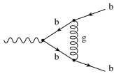
Figure 2: SM diagrams for the $Zbb$ vertex (Higgs sector excluded).

Figure 3: SM Higgs diagrams for the $Zbb$ vertex.

The calculation in Ref. [33] is in perfect agreement with the results of Refs. [27, 28] for both the $\tau$ lepton and the $b$ quark. Taking as input parameters $m_{\tau}=1.777$ GeV, $m_{b}=4.5$ GeV, $m_{t}=175$ GeV, $M_{Z}=91.19$ GeV, $s^{2}_{W}=0.232$, $\alpha=1/128$ and $\alpha_{s}=0.118$, the pure electroweak contributions are:

$$a^{w}_{\tau}[{\rm EW}] = (2.10+0.61~{}{\rm i})\times 10^{-6},$$ (19)

$$a^{w}_{b}[{\rm EW}] = [(1.1;\ 2.0;\ 2.4)-0.2~{}{\rm i}]\times 10^{-6},$$ (20)

for three different values of the Higgs mass (respectively $M_{H^{0}}=M_{Z}$, $2M_{Z}$ and $3M_{Z}$). Note that for the $\tau$ case the Higgs boson contribution has a very small impact, changing the final result by less than $1\%$ in the range of the Higgs boson masses considered. A much stronger dependence is observed for the $b$ case. The CKM matrix element $V_{tb}$ is taken equal to one and all the off-diagonal entries vanishing. The whole SM contribution (EW+QCD) for the $b$ quark is dominated by the gluon exchange:

$$a^{w}_{b}[{\rm SM}]=(-2.98+1.56~{}{\rm i})\times 10^{-4}.$$

This large enhancement is as expected by the replacement $\alpha\rightarrow\alpha_{s}$.

The only phase present in the SM, the $\delta_{\rm CKM}$, is not sufficient for generating one-loop contributions to the (W)EDM. One needs to go beyond the two–loop level [15]. A very crude estimate of the tiny three–loop SM contribution to the (W)EDM can be done using simple power counting arguments. For a general fermion with mass $m_{f}$ $d^{w}_{f}[{\rm SM}]$ is of the order of $eG_{F}m_{f}\alpha^{2}\alpha_{s}J/(4\pi)^{5}$ with $J=c_{1}c_{2}c_{3}s_{1}^{2}s_{2}s_{3}s_{\delta}$ being an invariant under reparameterizations of the CKM matrix [14]. For the $\tau$ lepton and the $b$ quark we have:

$$d^{w}_{\tau}[{\rm SM}]\raisebox{-3.69899pt}{~{}\shortstack{$<$ \\ [-0.07cm] $\sim$}}~{}1.5\times 10^{-19}\ \mu_{\tau}\qquad{\rm and}\qquad d^{w}_{b}[{\rm SM}]\raisebox{-3.69899pt}{~{}\shortstack{$<$ \\ [-0.07cm] $\sim$}}~{}1.5\times 10^{-18}\ \mu_{b}.$$ (21)

We use the scale unit $\mu_{f}\equiv e/2m_{f}$ (“magneton”) with $\mu_{\tau}\ (\mu_{b})=5.55\ (2.19)\times 10^{-15}\ e$cm, respectively.

3.2 The $\tau$ and $b$ AWMDMs in the MSSM

The particle content of the MSSM includes the SM spectrum, the SUSY partners and an extended Higgs sector consisting of two doublets. We assume implicitly R–parity conservation. The new non SM diagrams are depicted in Figs. 4 and 5.

Figure 4: MSSM Higgs diagrams for $Zbb$.

Figure 5: MSSM diagrams for $Zbb$.

They will be grouped into sets of diagrams including Higgs bosons, neutralinos, charginos and gluinos, as in Ref. [33]. All of them belong to the topologies of classes III, IV, V and VI.

The MSSM involves a large set of new parameters currently unknown but constrained by present experimental data. For sake of simplicity we assume the usual GUT relations for the soft–breaking gaugino mass terms,

$$\quad M_{1}=\frac{5}{3}\tan^{2}\theta_{W}M_{2}\ ,\quad M_{3}=\frac{\alpha_{s}}{\alpha}s^{2}_{W}M_{2}$$ (22)

and a common scalar fermion mass parameter. Moreover we restrict ourselves to two typical scenarios, low and high $\tan\beta$, set respectively to $\tan\beta=1.6$ and $\tan\beta=50$. We also assume generation–diagonal, not universal, trilinear soft–breaking terms in order to prevent large FCNC. We are left, for given values of $\tan\beta$, with the following free parameters: the gaugino mass parameter for the SU(2) sector $M_{2}$, the Higgs–higgsino mass parameter $\mu$, the mass of the pseudoscalar Higgs boson $M_{A}$, the common scalar lepton soft–breaking mass parameter $m_{\tilde{l}}$, the common scalar quark soft-breaking mass parameter $m_{\tilde{q}}$ and the trilinear soft–breaking terms $A_{f}$ (for $f=b,t$ or $\tau$). The conventions for couplings and mixing are extensively explained in the Appendices. In this Section all the supersymmetric parameters are taken real.

3.2.1 MSSM Higgs contribution to the AWMDMs

The MSSM $Zbb$ diagrams involving Higgs bosons are shown in Fig. 4. There $G^{0}$ and $G^{\pm}$ are the would–be–Goldstone bosons and $h$, $H$, $H^{\pm}$ and $A$ are the physical scalar and pseudoscalar MSSM Higgs bosons. Actually not all these diagrams contribute to the AWMDM: the class IV diagrams with neutral Higgs bosons (necessarily of opposite parity) identically vanish, also in the SM, due to the way their couplings to fermions (236–241,243) combine in (15). There are only three independent parameters involved in the Higgs sector: $\tan\beta$, the mass of the pseudoscalar $M_{A}$, and the common scalar fermion mass parameter $m_{\tilde{f}}$. The Higgs contribution decreases with growing $M_{A}$ and $m_{\tilde{f}}$, consistently with the decoupling theorem [38, 39].

The Higgs contribution to the Re($a^{w}_{\tau}$) coming from the diagrams of classes III and IV are proportional to $(m_{\tau}/M_{Z})^{4}\tan^{2}\beta$ and those from the diagrams of classes V and VI are proportional to $(m_{\tau}/M_{Z})^{2}$. Due to the fourth power suppression the sum is not very sensitive to $\tan\beta$. We obtain

$${\rm Re}\left(a^{w}_{\tau}[{\rm Higgs}]\right)=-0.3~{}(-0.4)\times 10^{-6}\quad\mbox{for}\quad\tan\beta=1.6~{}(50),$$

$m_{\tilde{q}}=250$ GeV and $M_{A}=100$ GeV. Assuming the present lower bounds for the masses of the Higgs bosons [40, 41] the only contribution to the Im($a^{w}_{\tau}$) can arise from class III diagrams and it is in general smaller than the SM one.

The same considerations apply for the Higgs contribution to the $b$ AWMDM. The only relevant difference is the presence of a dominant term proportional to $(m_{b}m_{t}/M_{Z}^{2})^{2}$. The Re($a^{w}_{b}$) is:

$${\rm Re}\left(a^{w}_{b}[{\rm Higgs}]\right)=-3.8~{}(+0.8)\times 10^{-6}\quad\mbox{ for }\quad\tan\beta=1.6~{}(50),$$

$m_{\tilde{q}}=250$ GeV and $M_{A}=100$ GeV. Again the contribution to the Im$(a^{w}_{b})$ is negligible.

3.2.2 Chargino contribution to the AWMDMs

There are two diagrams with charginos and scalar fermions (Fig. 5). In the region of MSSM parameters not ruled out by present experiments [41] charginos and scalar fermions cannot be pair produced in $Z$ decays. Therefore they can contribute only to the real part of the AWMDM. The free parameters involved are $\tan\beta$, $M_{2}$, $\mu$, $m_{\tilde{f}}$ (and $A_{t}$ in the $b$ case, since there is no mixing in the scalar neutrino sector). Increasing the scalar fermion common mass only produces decoupling of the scalar fermion from the spectrum. In the large $M_{2}$ and $|\mu|$ region also the charginos decouple.

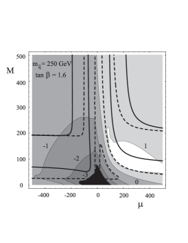
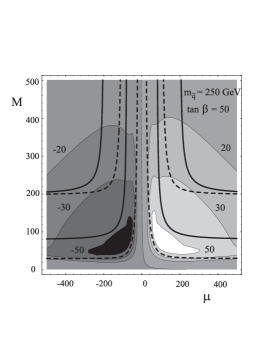
(a)	(b)

Figure 6: Re($a^{w}_{b}$[char]) for low (a) and high (b) $\tan\beta$ in units of $10^{-6}$ in the plane $M_{2}-\mu$. The contour solid-lines correspond to the lightest chargino masses $m_{\tilde{\chi}^{\pm}}=90$ and $200$ GeV and the contour dashed-lines correspond to the lightest neutralino masses $m_{\tilde{\chi}^{0}}=15$ and $100$ GeV. The common scalar quark mass parameter is fixed to $m_{\tilde{q}}=250$ GeV and $m^{t}_{LR}=0$. From [33].

The chargino contribution to the real part of the $\tau$ AWMDM is:

$${\rm Re}\left(a^{w}_{\tau}[{\rm char}]\right)=\pm 0.2~{}(\pm 7.0)\times 10^{-6}\quad\mbox{for}\quad\tan\beta=1.6~{}(50),$$

with $m_{\tilde{q}}=250$ GeV and $M_{2}=|\mu|=200$ GeV. The enhancement for higher $\tan\beta$ is due to the dependence of the chargino and neutralino couplings on the Higgs vacuum expectation values.

For the real part of the $b$ AWMDM one gets:

$${\rm Re}\left(a^{w}_{b}[{\rm char}]\right)=\pm 1.1~{}(\pm 33)\times 10^{-6}\quad\mbox{for}\quad\tan\beta=1.6~{}(50),$$

with $m_{\tilde{q}}=250$ GeV, $M_{2}=|\mu|=200$ GeV and $A_{t}=\mu\cot\beta$. The $\pm$ stands for ${\rm sign}(\mu)$. Varying the value of $A_{t}$ in the range $\pm\mu\cot\beta$ there is only a small effect in the AWMDM. We thus choose the value of $A_{t}$ that makes the off–diagonal entry of the $\tilde{t}$ scalar quarks mixing mass matrix vanish. In such a way the scalar fermion mass eigenstates are always physical. Fig. 6 shows the contour plot of the ${\rm Re}(a^{w}_{b}[{\rm char}])$ in the $M_{2}-\mu$ plane. The contour lines for fixed masses of the lightest chargino (90 and 200 GeV) and lightest neutralino (15 and 100 GeV) are also given for illustration. The contributions are enhanced by increasing $\tan\beta$. In the low $\tan\beta$ scenario the contribution is of order $10^{-6}$ (Fig. 6a), while in the high $\tan\beta$ scenario it becomes of order $10^{-5}$ (Fig. 6b). The contour plots for the $\tau$ AWMDM are similar to the $b$ quark ones but suppressed by factors between $m_{\tau}/m_{b}$ and $(m_{\tau}/m_{b})^{2}$ [see Eqs. (13) and (15)].

3.2.3 Neutralino contribution to the AWMDMs

The two diagrams involving neutralinos and scalar fermions are shown in Fig. 5. The scalar fermion masses are bounded by present experiments to be heavy but the neutralino masses can be lighter than half the mass of the $Z$ [41]. This allows for the possibility of a contribution to the imaginary part of the AWMDM through class III diagrams. A non negligible effect can arise only extremely near to the neutralino production threshold. The neutralino contribution to the AWMDM depends on $\tan\beta$, $M_{2}$, $\mu$, $m_{\tilde{f}}$, as well as the trilinear soft–breaking mass term $A_{f}$. No sizeable deviations due to changes in $A_{f}$ in the range $\pm\mu\tan\beta$ are observed. To avoid an unphysical mass for the fermion we take $m^{f}_{LR}=0$. The usual decoupling properties for scalar and fermions have been successfully checked.

For the real parts of the $\tau$ and $b$ AWMDM one gets:

$${\rm Re}\left(a^{w}_{\tau}[{\rm neut}]\right) = -0.02~{}(-0.4)\times 10^{-6},$$ (23)

$${\rm Re}\left(a^{w}_{b}[{\rm neut}]\right) = -0.2~{}(-10.5)\times 10^{-6}\quad\mbox{for}\quad\tan\beta=1.6~{}(50).$$ (24)

and $M_{2}=\mu=200$ GeV. Like in the chargino contributions the result is enhanced with increasing $\tan\beta$.

3.2.4 Gluino contribution to the $b$ AWMDM

In the case of the $b$ AWMDM one more diagram must be considered: the one with a gluino and two $\tilde{b}$ scalar quarks running in the loop. Due to the $\alpha\rightarrow\alpha_{s}$ replacement, we expect from the gluino sector a large contribution to the $b$ AWMDM. The present bounds on $\tilde{b}$ scalar quark masses [41] only allow a real contribution to the AWMDM. The free parameters are $\tan\beta$, $m_{\tilde{q}}$, $m_{\tilde{g}}$, $A_{b}$ and $\mu$. The last two affect the result only through the off–diagonal term of the $\tilde{b}$ scalar quark mass matrix $m^{b}_{LR}=A_{b}-\mu\tan\beta$. This parameter is responsible for the mixing in the $\tilde{b}$ sector and intervenes in association with the chirality flipping in the gluino internal line. Thus the contribution to the AWMDM is almost proportional to $m^{b}_{LR}$. We assume $\mu\tan\beta$ as typical scale for $m^{b}_{LR}$.

In Fig. 7 the gluino contribution to the $b$ AWMDM is displayed in the $m^{b}_{LR}-m_{\tilde{g}}$ plane. In the low $\tan\beta$ region (Fig. 7a) the value of $m^{b}_{LR}$ does not affect significantly the mass of the lightest $\tilde{b}$ scalar quark (always above 200 GeV). For zero gluino mass, only the term proportional to the mass of the $b$ quark provides a contribution. As we increase the gluino mass, the term proportional to $m_{\tilde{g}}$ dominates, especially for large $m^{b}_{LR}$, becoming again suppressed at high $m_{\tilde{g}}$ due to the gluino decoupling. For high $\tan\beta$ the behavior is analogous but larger values for the AWMDM can be obtained as shown in Fig. 7b (extremely high values of $m^{b}_{LR}$ are excluded due to unphysical $m^{2}_{\tilde{b}_{1}}<0$). Typical values are:

$${\rm Re}\left(a^{w}_{b}[{\rm glu}]\right) = -1.1\times 10^{-6}\qquad{\rm for}~{}\tan\beta=1.6,~{}m^{b}_{LR}=200~{}{\rm GeV},$$ (25)

$${\rm Re}\left(a^{w}_{b}[{\rm glu}]\right) = -18.9\times 10^{-6}\qquad{\rm for}~{}\tan\beta=50,~{}m^{b}_{LR}=7~{}{\rm TeV},$$ (26)

with the gluino mass fixed to $m_{\tilde{g}}=200$ GeV. Using the GUT constraint (22) higher values for the gluino mass ($m_{\tilde{g}}\equiv M_{3}$) seem more likely and in this case the results in Eqs. (25, 26) are approximately reduced linearly with $m_{\tilde{g}}$.

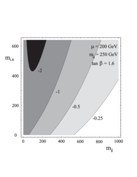
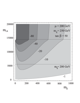
(a)	(b)

Figure 7: Re($a^{w}_{b}$[glu]) low (a) and high (b) $\tan\beta$ in units of $10^{-6}$ in the plane $m^{b}_{LR}-m_{\tilde{g}}$. The common scalar quark mass parameter is fixed to $m_{\tilde{q}}=250$ GeV. The region above the upper horizontal line is unphysical ($m^{2}_{\tilde{b}_{1}}<0$). From [33].

3.2.5 MSSM total contribution to the AWMDMs

The imaginary parts of the $\tau$ lepton and $b$ quark AWMDM are provided only by the diagrams with Higgs bosons and neutralinos. The total contribution in a reasonable region of the MSSM parameter can reach at maximum $10^{-6}$ and is typically lower than the corresponding SM contribution.

The real part is dominated by the chargino and the gluino sectors, when present. It is roughly proportional to $\tan\beta$. The total contribution can reach the values:

$$|{\rm Re}(a^{w}_{\tau}[{\rm MSSM}])| \sim 0.5~{}(7)\times 10^{-6},$$ (27)

$$|{\rm Re}(a^{w}_{b}[{\rm MSSM}])| \sim 2~{}(50)\times 10^{-6}$$ (28)

for $\tan\beta=1.6~{}(50)$ respectively. In the low $\tan\beta$ scenario the MSSM contribution to the AWMDM is of the same order than in the SM (19,20). More interesting is the high $\tan\beta$ scenario where the MSSM contribution to the real part can reach values one order of magnitude higher than the pure electroweak SM contribution, especially in the $b$ quark case (20), but still a factor five below the standard QCD contribution (3.1).

3.3 The $\tau$ and $b$ WEDMs in the MSSM

Eqs. (9–18) show that for having non–vanishing contribution to the WEDMs one has to deal with complex couplings. Many of the parameters in the SUSY Lagrangian can be complex but not all the phases originated are physical. Some of them can be absorbed by a redefinition of the MSSM fields (see App. B for a complete discussion of the procedure). Our choice of CP–violating phases is: $\varphi_{\mu}\equiv{\rm arg}(\mu)$, $\varphi_{\tilde{f}}\equiv{\rm arg}(m^{f}_{\rm LR})$ ($f=\tau,\ t,\ b$) with $m^{t}_{\rm LR}\equiv A_{t}-\mu^{*}\cot\beta$ and $m^{\tau,b}_{\rm LR}\equiv A_{\tau,b}-\mu^{*}\tan\beta$.

Since the MSSM contains a CP–conserving Higgs sector and the SM provides contributions to the (W)EDMs beyond two loops, the relevant diagrams are the genuine SUSY graphs of classes III and IV [35].

3.3.1 Chargino contribution to the WEDM

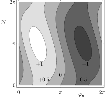
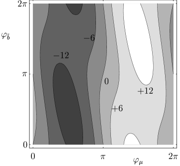
(a)	(b)

Figure 8: Re($d^{w}_{b}$[char]) for low $\tan\beta$ (a) and Re($d^{w}_{b}$[neut]) for high $\tan\beta$ (b) in the plane $\varphi_{\tilde{f}}-\varphi_{\mu}$, in units of $10^{-6}\ \mu_{b}$ with $M_{2}=|\mu|=m_{\tilde{q}}=250$ GeV. The mixing $|m^{t}_{LR}|=|\mu|\cot\beta$ and $|m^{b}_{LR}|=|\mu|\tan\beta$, respectively. From [35].

There is only one phase, $\varphi_{\mu}$, involved in the chargino contribution to the $\tau$ WEDM, as there is no mixing in the scalar neutrino sector. The result grows with $\tan\beta$. It also depends on the common scalar lepton mass (whose effect consists of diminishing the result through the tensor integrals) and the $|\mu|$ and $M_{2}$ mass parameters. Taking $M_{2}=|\mu|=m_{\tilde{l}}=250$ GeV one obtains:

$${\rm Re}\left(d^{w}_{\tau}[{\rm char}]\right)=0.18~{}(5.52)\times 10^{-6}~{}\mu_{\tau}\quad{\rm for}\quad\tan\beta=1.6~{}(50)$$ (29)

in the limit $\varphi_{\mu}=\pi/2$, for which the WEDM takes the largest value.

Two CP-violating phases are involved in the $b$ case: $\varphi_{\mu}$ and $\varphi_{\tilde{t}}$. In Fig. 8a the dependence on these phases is shown, for $M_{2}=|\mu|=m_{\tilde{q}}=250$ GeV, $|m^{t}_{LR}|=|\mu|\cot\beta$ and both low and high $\tan\beta$ scenarios. The maximum effect on the WEDM is obtained for $\varphi_{\mu}=\pi/2$ and $\varphi_{\tilde{t}}=\pi$. One gets up to

$${\rm Re}\left(d^{w}_{b}[{\rm char}]\right)=1.17~{}(27.1)\times 10^{-6}~{}\mu_{b}\quad{\rm for}\quad\tan\beta=1.6~{}(50).$$ (30)

In the high $\tan\beta$ scenario our assumed $|m^{t}_{LR}|$ takes a small value and the dependence on $\varphi_{\tilde{t}}$ tends to disappear. To have an idea of the maximum value achievable for the chargino contribution, we show in Fig. 9 the dependence on $M_{2}$ and $|\mu|$ for $\varphi_{\mu}=\pm\pi/2$ and $m^{t}_{LR}=0$ with the previous value for the common scalar quark mass parameter. Assuming the present bounds on the chargino masses [41], there is no contribution to the imaginary part of the $\tau$ and $b$ WEDM.

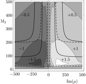
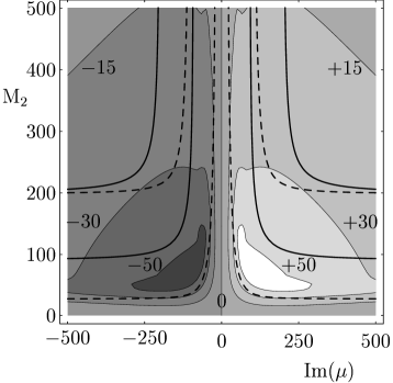
(a)	(b)

Figure 9: Re($d^{w}_{b}$[char]) for low (a) and high (b) $\tan\beta$ in the plane $M_{2}-$Im$(\mu)$, in units of $10^{-6}\ \mu_{b}$ with $|\sin\varphi_{\mu}|=1$ and $m_{\tilde{q}}=250$ GeV. The mixing $|m^{t}_{LR}|=0$. The contour solid-lines correspond to the lightest chargino masses $m_{{\tilde{\chi}}^{\pm}_{1}}=80$ and $200$ GeV and the contour dashed-lines correspond to the lightest neutralino masses $m_{{\tilde{\chi}}^{0}_{1}}=15$ and $100$ GeV. From [35].

3.3.2 Neutralino contribution to the WEDMs

Now both $\varphi_{\mu}$ and $\varphi_{\tilde{\tau}}$ contribute. Assuming that $|m^{\tau}_{LR}|$ is of the order of $|\mu|\tan\beta$ or below, there is no large influence of $\varphi_{\tilde{\tau}}$ on the neutralino contribution, for both low and high $\tan\beta$. This contribution is roughly proportional to $\sin\varphi_{\mu}$ regardless of the value of $\varphi_{\tilde{\tau}}$. Taking $\varphi_{\mu}=\pi/2$, $M_{2}=|\mu|=250$ GeV and $m_{\tilde{l}}=250$ GeV one finds:

$${\rm Re}\left(d^{w}_{\tau}[{\rm neut}]\right)=-0.01~{}(-0.25)\times 10^{-6}~{}\mu_{\tau}\quad{\rm for}\quad\tan\beta=1.6~{}(50).$$ (31)

The two relevant CP-violating phases for the neutralino contribution to the $b$ WEDM are: $\varphi_{\mu}$ and $\varphi_{\tilde{b}}$. As before, the most important effect from $\varphi_{\tilde{b}}$ arises when the off–diagonal term is larger, which in this case corresponds to high $\tan\beta$, as the trilinear soft breaking parameter is taken to be of the order of $|\mu|\tan\beta$. The maximum value for the neutralino contribution occurs for $\varphi_{\mu}=\varphi_{\tilde{b}}=\pi/2$ (Fig. 8b). The total contribution increases with $\tan\beta$. Thus taking $M_{2}=|\mu|=m_{\tilde{q}}=250$ GeV and $|m^{b}_{LR}|=|\mu|\tan\beta$ one gets:

$${\rm Re}\left(d^{w}_{b}[{\rm neut}]\right)=-0.29~{}(-12.6)\times 10^{-6}~{}\mu_{b}\quad{\rm for}\quad\tan\beta=1.6~{}(50).$$ (32)

For presently non excluded masses of the neutralinos [41] there can be a contribution to the imaginary part of the order of $10^{-6}\ \mu_{f}$.

3.3.3 Gluino contribution to the $b$ WEDM

The gluino contribution is affected only by $m^{b}_{LR}$, $m_{\tilde{q}}$ and the gaugino mass $m_{\tilde{g}}$. Therefore the maximum value occurs for $\varphi_{\tilde{b}}=\pi/2$. The mixing in the $\tilde{b}$ sector is determined by $m^{b}_{LR}$ and intervenes in the contribution due to chirality flipping in the gluino internal line (the contribution proportional to $m_{\tilde{g}}$). The contribution to the WEDM is enhanced by the largest values of $|m^{b}_{LR}|$ compatible with an experimentally not excluded mass for the lightest $\tilde{b}$ scalar quark. For zero gluino mass, only the term proportional to the mass of the $b$ quark provides a contribution. Thus for $\varphi_{\tilde{b}}=\pi/2$ one gets:

$${\rm Re}\left(d^{w}_{b}[{\rm gluinos}]\right)=0.26~{}(9.31)\times 10^{-6}~{}\mu_{b}\quad{\rm for}\quad\tan\beta=1.6~{}(50),$$ (33)

$|m^{b}_{LR}|=|\mu|\tan\beta$, $M_{2}=|\mu|=m_{\tilde{q}}=250$ GeV and $m_{\tilde{g}}\equiv M_{3}$ fulfilling the GUT relation (22). There exists the possibility for a gluino contribution to the imaginary part of the $b$ WEDM if the hypothesis of light gluino is not discarded.

3.3.4 MSSM total contribution to the WEDMs

The Higgs sector does not contribute and chargino diagrams are more important than neutralino ones. Gluinos are also involved in the $b$ case and compete in importance with charginos. In the most favorable configuration of CP-violating phases and for values of the rest of the parameters still not excluded by experiments, these WEDMs can be as much as twelve orders of magnitude larger than the SM estimates (21):

$$|{\rm Re}(d^{w}_{\tau})| < \sim 0.2~{}(6)\times 10^{-6}~{}\mu_{\tau}$$   [-0.07cm] (34)

$$|{\rm Re}(d^{w}_{b})| < \sim 2~{}(35)\times 10^{-6}~{}\mu_{b}$$   [-0.07cm] (35)

There may be a contribution to the imaginary part if the neutralinos are light but this contribution is at least one order of magnitude smaller than the real part of the $\tau$ or $b$ WEDM.

3.4 Cancellation of the dipole moments in the supersymmetric limit

A general $Vff$ interaction is restricted to the form (2) by Lorentz invariance. Since the Lorentz algebra is a subalgebra of the supersymmetry algebra, this interaction is even more constrained in a theory with unbroken supersymmetry. In fact, supersymmetric sum rules are derived that relate the electric and magnetic multipole moments of any irreducible $N=1$ supermultiplet [43]. Applied to the $Vff$ interaction between a vector boson coupling to a conserved current and the fermionic component of a chiral multiplet, these sum rules force the gyromagnetic ratio to be $g_{f}=2$ and forbid an electric dipole moment:

$$a^{V}_{f}=d^{V}_{f}=0.$$ (36)

The Lagrangian of the MSSM is supersymmetric when the soft–breaking terms are removed. For non zero value of the $\mu$ parameter the Higgs potential has only a trivial minimum. Therefore to keep the particles massive and supersymmetry preserved at the same time the choice $\mu=0$ is necessary. Then the Higgs potential is positive semi–definite and it has degenerate minima corresponding to $v\equiv v_{1}=v_{2}$ ($\tan\beta=1$). The value of $M_{A}=0$ follows from such a configuration. Finally the value of the common $v$ is fixed by the phenomenology: the muon decay constant and the gauge boson masses.

In this supersymmetric limit the above mentioned sum rules are valid and the magnetic and electric dipole form factors have to cancel. To verify our expressions we checked this for the AWMDM of the $b$ quark [35]. Choosing the parameters $A_{b}=A_{t}=M_{2}=M_{3}=0$, $\mu=0$, $\tan\beta=1$ and $M_{A}=0$, the SM gauge boson contribution to $a^{w}_{b}$ [28] is indeed cancelled by the MSSM correction including the two Higgs doublets: the gluon and gluino contribution cancel among themselves and the neutralinos and charginos cancel the gauge boson and Higgs contributions.

4 SM and MSSM predictions for the top quark dipole form factors

4.1 SM

The electroweak contributions to the magnetic and weak–magnetic dipole form factors for off–shell gauge bosons are gauge dependent. The pinch technique [44] could be used to construct gauge–parameter independent magnetic dipoles in the class of $R_{\xi}$ gauges [45, 32] but the prescription is not unique [46] and these quantities cannot be observable by themselves. The QCD contributions (gluon exchange) to the $t$ (W)MDFF are gauge independent and comparable in size to the electroweak predictions at $\sqrt{s}=500$ GeV in the ’t Hooft–Feynman gauge due to the large mass of the $t$ quark [32].

There is no contribution to the electric and weak–electric dipole form factors to one loop in the SM.

4.2 MSSM

The triangle diagrams with SUSY particles are gauge independent by themselves (no gauge or Goldstone bosons involved) but the ones including Higgs scalars and gauge bosons in the loop are not sufficient to keep the gauge invariance in the case of the magnetic dipole form factor. The CP–violating dipole form factors (electric and weak–electric) for which the Higgs sector of the MSSM is irrelevant, on the other hand, can be regarded as gauge independent quantities. These form factors have also been considered in [36].

We investigate the SUSY contributions to the $t$ electric and weak–electric dipole form factors performing a parameter scan for which a fixed value $\sqrt{s}=500$ GeV has been chosen. It is important to point out that the region of the supersymmetric parameter space that provides the maximal contributions varies with $s$ due to threshold effects. We scan the mass parameters $M_{2}$ and $|\mu|$ in a broad range and the CP–violating phases: $\varphi_{\mu}$, $\varphi_{\tilde{t}}$ and $\varphi_{\tilde{b}}$ (see Figs. 10 and 11). The gluino mass is given by the GUT constraint (22). We adopt a fixed value for the common scalar quark mass $m_{\tilde{q}}=200$ GeV: this is a plausible intermediate value; larger values decrease the effects. Finally, the moduli of the off–diagonal terms in the $\tilde{t}$ and $\tilde{b}$ mass matrices are also chosen at fixed values $|m^{t}_{LR}|=|m^{b}_{LR}|=200$ GeV, to reduce the number of free parameters. The results are expressed in $t$ magnetons $\mu_{t}\equiv e/2m_{t}=5.64\times 10^{-17}\ e$cm.

The MSSM contributions to the top quark EDFF and WEDFF include:

4.2.1 Neutralinos and ${\tilde{t}}$ scalar quarks

Re$\{d^{\gamma}_{t}[{\tilde{\chi}}^{0}]\}$	Im$\{d^{\gamma}_{t}[{\tilde{\chi}}^{0}]\}$
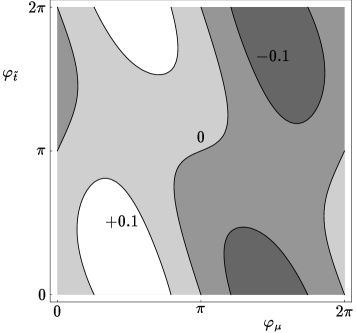
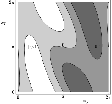
Re$\{d^{Z}_{t}[{\tilde{\chi}}^{0}]\}$	Im$\{d^{Z}_{t}[{\tilde{\chi}}^{0}]\}$

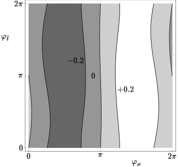
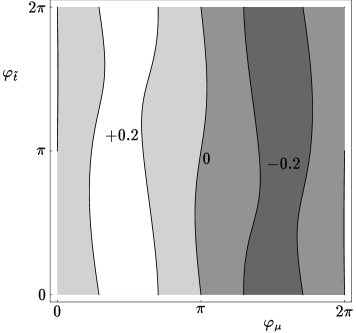
Figure 10: Neutralino contribution to the real and imaginary parts of the $t$ EDFF and WEFF [in $10^{-3}\mu_{t}$ units] in the plane $\varphi_{\tilde{t}}-\varphi_{\mu}$ for $\tan\beta=1.6$ and the reference values $M_{2}=|\mu|=|m^{t}_{LR}|=200$ GeV at $\sqrt{s}=500$ GeV.

They provide typically small contributions but quite sensitive to the value of both the phases involved, $\varphi_{\mu}$ and $\varphi_{\tilde{t}}$ (Fig. 10).

The results are larger for low $\tan\beta$ since the chirality flipping mass terms are dominated by the $t$ quark, yielding a term proportional to $m_{t}\cot\beta$. A term proportional to the neutralino masses is also present as well as a negligible one proportional to $m_{b}\tan\beta$. The contributing diagrams belong to the classes III and IV for the $Z$ case and only to class IV for the $\gamma$ case, as the neutralinos do not couple to photons.

As a reference we take the representative values $M_{2}=|\mu|=200$ GeV and $\varphi_{\mu}=-\varphi_{\tilde{t}}=\pi/2$. For these inputs the results are

$$d^{\gamma}_{t}[{\tilde{\chi}}^{0}] = (\ 0.080+0.081\ {\rm i})\times 10^{-3}\ \mu_{t}$$ (37)

$$d^{Z}_{t}[{\tilde{\chi}}^{0}] = (-0.324+0.223\ {\rm i})\times 10^{-3}\ \mu_{t}$$ (38)

4.2.2 Charginos and ${\tilde{b}}$ scalar quarks

Re$\{d^{\gamma}_{t}[{\tilde{\chi}}^{\pm}]\}$	Im$\{d^{\gamma}_{t}[{\tilde{\chi}}^{\pm}]\}$
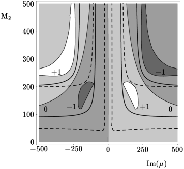
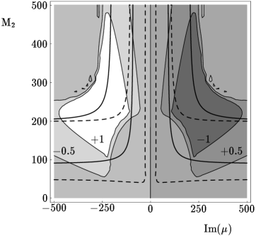
Re$\{d^{Z}_{t}[{\tilde{\chi}}^{\pm}]\}$	Im$\{d^{Z}_{t}[{\tilde{\chi}}^{\pm}]\}$

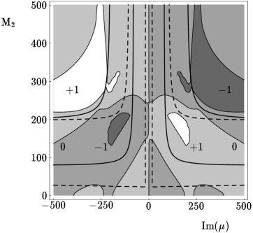
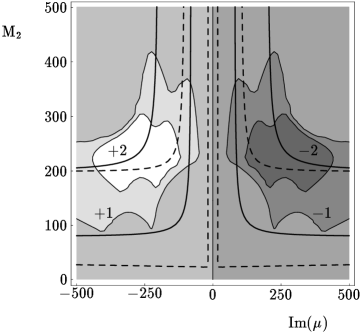
Figure 11: Chargino contribution to the real and imaginary parts of the $t$ EDFF and WEFF [in $10^{-3}\mu_{t}$ units] in the plane $M_{2}-{\rm Im}(\mu)$ for $\tan\beta=1.6$, $|m^{b}_{LR}|=200$ GeV and $\varphi_{\tilde{b}}=\pi/2$ at $\sqrt{s}=500$ GeV. The lower (upper) solid isolines correspond to $m_{\tilde{\chi}^{\pm}_{1}}=90\ (200)$ GeV and the dashed isolines to $m_{\tilde{\chi}^{0}_{1}}=25\ (100)$ GeV.

As in the case of the neutralinos, the influence of chargino diagrams is enhanced for low $\tan\beta$.

The results depend very little on $\varphi_{\tilde{b}}$ and mainly on $\varphi_{\mu}$, the maxima being close to $\varphi_{\mu}=\pm\pi/2$. For increasing $\tan\beta$ the dependence on $\varphi_{\tilde{b}}$ grows, as it comes with a factor proportional to $m_{b}\tan\beta$.

The chargino contributions are the most important ones. In Fig. 11 the dependence on Im$(\mu)$ and $M_{2}$ is displayed for $\tan\beta=1.6$. The only relevant CP–violating phase here has been set to the most favorable case, $\varphi_{\mu}=\pi/2$ (the negative values of Im$(\mu)$ correspond to $\varphi_{\mu}=-\pi/2$). The symmetry with respect to Im$(\mu)=0$ in Fig. 11 reflects the approximate independence of $\varphi_{\tilde{b}}$, here set to $\pi/2$. The same does not happen for the neutralino contributions for a fixed value of $\varphi_{\tilde{t}}\neq 0,\pi$ in the plane $M_{2}-{\rm Im}(\mu)$. The plots of Fig. 11 exhibit a tendency to decoupling of the supersymmetric effects for increasing values of the mass parameters. The isolines for a couple of masses of the lightest charginos and neutralinos in the same plane are also given for orientation. The current LEP2 experimental lower limits are $m_{\tilde{\chi}^{0}_{1}}>25$ GeV and $m_{\tilde{\chi}^{\pm}_{1}}>90$ GeV [41].

The chargino contributions for the values $M_{2}=|\mu|=200$ GeV and $\varphi_{\mu}=\pi/2$ are

$$d^{\gamma}_{t}[{\tilde{\chi}}^{\pm}] = (0.869-1.870\ {\rm i})\times 10^{-3}\ \mu_{t}$$ (39)

$$d^{Z}_{t}[{\tilde{\chi}}^{\pm}] = (0.793-2.524\ {\rm i})\times 10^{-3}\ \mu_{t}$$ (40)

4.2.3 Gluinos and ${\tilde{t}}$ scalar quarks

Their effect is roughly proportional to $|m^{t}_{LR}|\sin\varphi_{\tilde{t}}$ times a chirality flipping fermion mass, either $m_{t}$ or $M_{3}$ (the gluino mass). It is damped for heavy gluinos circulating in the loop and also for large scalar quark masses (decoupling). Both terms have opposite sign to Im($m^{t}_{LR}$) and the one proportional to the gluino mass dominates.

The result for $M_{2}=200$ GeV and $\varphi_{\tilde{t}}=-\pi/2$ is

$$d^{\gamma}_{t}[{\tilde{g}}] = (0.457+0.170\ {\rm i})\times 10^{-3}\ \mu_{t}$$ (41)

$$d^{Z}_{t}[{\tilde{g}}] = (0.155+0.059\ {\rm i})\times 10^{-3}\ \mu_{t}$$ (42)

4.2.4 Total contribution

In view of these results, we establish a set of SUSY parameters and phases for which nearly all the contributions sum up constructively at $\sqrt{s}=500$ GeV. Our choice is

$$\mbox{Reference Set }\#1: \tan\beta=1.6$$ (43)

$$M_{2}=|\mu|=m_{\tilde{q}}=|m^{t}_{LR}|=|m^{b}_{LR}|=200\mbox{ GeV}$$

$$\varphi_{\mu}=-\varphi_{\tilde{t}}=-\varphi_{\tilde{b}}=\pi/2,$$

for which the $t$ EDFF and WEFF reach the values:

$$d^{\gamma}_{t} = (1.407-1.618\ {\rm i})\times 10^{-3}\ \mu_{t}$$ (44)

$$d^{Z}_{t} = (0.624-2.242\ {\rm i})\times 10^{-3}\ \mu_{t},$$ (45)

at $\sqrt{s}=500$ GeV. To illustrate how the maximum effects appear we display in Fig. 12 the individual contributions as a function of $\sqrt{s}$. The masses of the supersymmetric partners in the loops are such that there are threshold enhancements in the vicinity of $\sqrt{s}=500$ GeV.

Figure 12: The different contributions to the $t$ (W)EDFF [in $10^{-3}\mu_{t}$ units] for the reference set of SUSY parameters of Eq. (43).

5 Observables at the $Z$ resonance: the $\tau$ lepton case

We analyze below a set of observables sensitive to the weak dipole moments at the $Z$ peak. In this environment the effects of electromagnetic dipole moments to the process $e^{+}e^{-}\to f\bar{f}$ are negligible, as the pair production proceeds through the $Z$ resonance. The $\gamma-$exchange and box diagrams are suppressed.

5.1 The $Z$ width

The $Z$ width is given in terms of generic vertex form factors by

$$\Gamma(Z\to f\bar{f}) = \frac{G_{F}M^{3}_{Z}}{6\sqrt{2}\pi}\sqrt{1-\frac{4m^{2}_{f}}{M^{2}_{Z}}}\Bigg{[}v^{2}_{f}\left(1+\frac{2m^{2}_{f}}{M^{2}_{Z}}\right)+a^{2}_{f}\left(1-\frac{4m^{2}_{f}}{M^{2}_{Z}}\right)$$ (46)

$$-6v_{f}s_{W}c_{W}{\rm Re}(a^{w}_{f})+4s_{W}^{2}c_{W}^{2}|a^{w}_{f}|^{2}\left(\frac{M^{2}_{Z}}{8m^{2}_{f}}+1\right)$$

$$+2s_{W}^{2}c_{W}^{2}|\hat{d}^{w}_{f}|^{2}\left(\frac{M^{2}_{Z}}{4m^{2}_{f}}-1\right)\Bigg{]}\ ,$$

where we have introduced the dimensionless parameter $\hat{d}^{w}_{f}\equiv 2m_{f}d^{w}_{f}/e$ for simplicity.

From the previous expression one observes that the real part of the AWMDM contributes linearly to the total width (although it is not necessarily the dominant term in the $\tau$ case for $a^{w}_{\tau}$ near the experimental upper limit, due to the small value of $v_{\tau}$ and the $M^{2}_{Z}/m^{2}_{\tau}$ enhancement factor). The WEDM contributes only quadratically to the total $Z$ width.

One might get some upper bounds on Re$(a^{w}_{f})$ and $|d^{w}_{f}|$ from the $Z$ partial widths measurements at LEP and SLC using the previous expressions. Actually this is not the most appropriate way to put limits to the dipoles as much information is integrated out. Moreover the weak–magnetic and weak–electric contributions cannot be disentangled and some other effects can interfere the measurements. In contrast, the differential cross section for the production of polarized fermion pairs contains all the ingredients needed and is the starting point for the construction of more specific observables.

5.2 The differential cross section $e^{-}e^{+}\to Z\to f\bar{f}$

The differential cross section for $e^{-}e^{+}\to f({\mathbf{s}_{\mathbf{1}}})\bar{f}({\mathbf{s}_{\mathbf{2}}})$ with polarized final fermions can be written as a sum of spin independent, single–spin dependent and spin–spin correlation contributions as

$$\frac{{\rm d}\sigma}{{\rm d}\Omega_{f}}({\mathbf{s}_{\mathbf{1}}},{\mathbf{s}_{\mathbf{2}}})=\frac{{\rm d}\sigma^{0}}{{\rm d}\Omega_{f}}+\frac{{\rm d}\sigma^{S}}{{\rm d}\Omega_{f}}({\mathbf{s}_{\mathbf{1}}}\oplus{\mathbf{s}_{\mathbf{2}}})+\frac{{\rm d}\sigma^{C}}{{\rm d}\Omega_{f}}({\mathbf{s}_{\mathbf{1}}}\otimes{\mathbf{s}_{\mathbf{2}}})\ ,$$ (47)

where ${\mathbf{s}_{\mathbf{1}}}$ (${\mathbf{s}_{\mathbf{2}}}$) are the polarization vectors of the fermion (antifermion). We choose a reference frame in which the $z$–axis points in the direction of the outgoing fermion and the $x$–$z$ plane contains both the incoming electron and the outgoing fermion. The polar angle $\theta_{f}$ is the angle between $e^{-}$ and the outgoing fermion. The azimuthal angle of the fermion can be integrated over, as the electron and positron are assumed unpolarized. The masses of the electron and positron will be neglected, as well as the quadratic terms in the anomalous couplings. The spin–correlation terms do not contribute when the polarization of only one of the two fermions is analyzed.

In terms of the final fermion velocity $\beta$, the dilatation factor $\gamma=M_{Z}/2m_{f}=(1-\beta^{2})^{-1/2}$ in the overall c.m.s. and the polarization vectors ${\bf s^{*}_{1,2}}$ of fermion and antifermion in their rest frames, the differential cross section $e^{-}e^{+}\to Z\to f\bar{f}$ (exactly on the Z resonance) reads

$$\frac{{\rm d}\sigma^{0}}{{\rm d}\cos\theta_{f}} = \frac{\alpha^{2}\beta N^{f}_{C}}{(4s_{W}c_{W})^{4}}\frac{1}{\Gamma^{2}_{Z}}\times\Bigg{\{}\ \ (v^{2}_{e}+a^{2}_{e})[v^{2}_{f}(2-\beta^{2}\sin^{2}\theta_{f})$$ (48)

$$\hskip 93.89418pt+a^{2}_{f}\beta^{2}(1+\cos^{2}\theta_{f})]+8v_{e}a_{e}v_{f}a_{f}\beta\cos\theta_{f}$$

$$-8s_{W}c_{W}{\rm Re}(a^{w}_{f})\ [(v_{e}^{2}+a_{e}^{2})v_{f}+2v_{e}a_{e}a_{f}\beta\cos\theta_{f}]\ \Bigg{\}}\ ,$$

$$\frac{{\rm d}\sigma^{S}}{{\rm d}\cos\theta_{f}} = \frac{\alpha^{2}\beta N^{f}_{C}}{(4s_{W}c_{W})^{4}}\frac{2s_{W}c_{W}}{\Gamma^{2}_{Z}}$$ (49)

$$\times[\ ({\mathbf{s}^{\mathbf{*}}_{\mathbf{1}}}+{\mathbf{s}^{\mathbf{*}}_{\mathbf{2}}})_{x}X_{+}+({\mathbf{s}^{\mathbf{*}}_{\mathbf{1}}}+{\mathbf{s}^{\mathbf{*}}_{\mathbf{2}}})_{y}Y_{+}+({\mathbf{s}^{\mathbf{*}}_{\mathbf{1}}}+{\mathbf{s}^{\mathbf{*}}_{\mathbf{2}}})_{z}Z_{+}$$

$$\ \ +({\mathbf{s}^{\mathbf{*}}_{\mathbf{1}}}-{\mathbf{s}^{\mathbf{*}}_{\mathbf{2}}})_{x}X_{-}+({\mathbf{s}^{\mathbf{*}}_{\mathbf{1}}}-{\mathbf{s}^{\mathbf{*}}_{\mathbf{2}}})_{y}Y_{-}+({\mathbf{s}^{\mathbf{*}}_{\mathbf{1}}}-{\mathbf{s}^{\mathbf{*}}_{\mathbf{2}}})_{z}Z_{-}\ ]\ ,$$

with

$$X_{+} = \Bigg{\{}-\frac{1}{\gamma s_{W}c_{W}}[2v_{e}a_{e}v^{2}_{f}+(v_{e}^{2}+a_{e}^{2})v_{f}a_{f}\beta\cos\theta_{f}]$$ (50)

$$\ +2\gamma{\rm Re}(a^{w}_{f})\ [2v_{e}a_{e}v_{f}(2-\beta^{2})+(v_{e}^{2}+a_{e}^{2})a_{f}\beta\cos\theta_{f}]\Bigg{\}}\sin\theta_{f}\ ,$$

$$Y_{+} = -2\gamma\beta{\rm Im}(a^{w}_{f})\ [2v_{e}a_{e}a_{f}+(v_{e}^{2}+a_{e}^{2})v_{f}\beta\cos\theta_{f}]\sin\theta_{f}\ ,$$ (51)

$$Z_{+} = -\frac{1}{s_{W}c_{W}}[(v_{e}^{2}+a_{e}^{2})v_{f}a_{f}\beta(1+\cos^{2}\theta_{f})+2v_{e}a_{e}(v^{2}_{f}+a^{2}_{f}\beta^{2})\cos\theta_{f}]$$ (52)

$$+2{\rm Re}(a^{w}_{f})\ [4v_{e}a_{e}v_{f}\cos\theta_{f}+(v_{e}^{2}+a_{e}^{2})a_{f}\beta(1+\cos^{2}\theta_{f})]\ ,$$

$$X_{-} = 2\gamma\beta{\rm Im}(\hat{d}^{w}_{f})\ [(v_{e}^{2}+a_{e}^{2})v_{f}\cos\theta_{f}+2v_{e}a_{e}a_{f}\beta]\sin\theta_{f}\ ,$$ (53)

$$Y_{-} = 2\gamma\beta{\rm Re}(\hat{d}^{w}_{f})\ [2v_{e}a_{e}v_{f}+(v_{e}^{2}+a_{e}^{2})a_{f}\beta\cos\theta_{f}]\sin\theta_{f}\ ,$$ (54)

$$Z_{-} = -2\beta{\rm Im}(\hat{d}^{w}_{f})\ (v_{e}^{2}+a_{e}^{2})v_{f}\sin^{2}\theta_{f}\ ,$$ (55)

and

$$\frac{{\rm d}\sigma^{C}}{{\rm d}\cos\theta_{f}} = \frac{\alpha^{2}\beta N^{f}_{C}}{(4s_{W}c_{W})^{4}}\frac{1}{\Gamma^{2}_{Z}}\ [\ s_{xx}C_{xx}+s_{yy}C_{yy}+s_{zz}C_{zz}$$ (56)

$$+(s_{xy}+s_{yx})C^{+}_{xy}+(s_{xz}+s_{zx})C^{+}_{xz}+(s_{yz}+s_{zy})C^{+}_{yz}$$

$$+({\mathbf{s}^{\mathbf{*}}_{\mathbf{1}}}\times{\mathbf{s}^{\mathbf{*}}_{\mathbf{2}}})_{x}C^{-}_{yz}+({\mathbf{s}^{\mathbf{*}}_{\mathbf{1}}}\times{\mathbf{s}^{\mathbf{*}}_{\mathbf{2}}})_{y}C^{-}_{xz}+({\mathbf{s}^{\mathbf{*}}_{\mathbf{1}}}\times{\mathbf{s}^{\mathbf{*}}_{\mathbf{2}}})_{z}C^{-}_{xy}\ ]\ ,$$

with

$$C_{xx} = (v^{2}_{e}+a^{2}_{e})[v^{2}_{f}(2-\beta^{2})-a^{2}_{f}\beta^{2}]\sin^{2}\theta_{f}$$ (57)

$$-8s_{W}c_{W}{\rm Re}(a^{w}_{f})\ (v_{e}^{2}+a_{e}^{2})v_{f}\sin^{2}\theta_{f}\ ,$$

$$C_{yy} = -(v_{e}^{2}+a_{e}^{2})(v_{f}^{2}-a_{f}^{2})\beta^{2}\sin^{2}\theta_{f}\ ,$$ (58)

$$C_{zz} = (v^{2}_{e}+a^{2}_{e})[v^{2}_{f}(2+\beta^{2}\sin^{2}\theta_{f})-a^{2}_{f}\beta^{2}(1+\cos^{2}\theta_{f})]$$ (59)

$$+8v_{e}a_{e}v_{f}a_{f}\beta\cos\theta_{f}$$

$$-2s_{W}c_{W}{\rm Re}(a^{w}_{f})\ [4(v_{e}^{2}+a_{e}^{2})v_{f}\cos^{2}\theta_{f}+8v_{e}a_{e}a_{f}\beta\cos\theta_{f}]\ ,$$

$$C^{+}_{xy} = 4s_{W}c_{W}\beta{\rm Im}(a^{w}_{f})\ (v_{e}^{2}+a_{e}^{2})a_{f}\sin^{2}\theta_{f}\ ,$$ (60)

$$C^{+}_{xz} = \Bigg{\{}\ \frac{1}{\gamma}[(v_{e}^{2}+a_{e}^{2})v^{2}_{f}\cos\theta_{f}+2v_{e}a_{e}v_{f}a_{f}\beta]$$ (61)

$$-4s_{W}c_{W}\gamma{\rm Re}(a^{w}_{f})\ [(v_{e}^{2}+a_{e}^{2})v_{f}(2-\beta^{2})\cos\theta_{f}$$

$$\hskip 93.89418pt+2v_{e}a_{e}a_{f}\beta]\Bigg{\}}\sin\theta_{f},$$

$$C^{+}_{yz} = 4s_{W}c_{W}\gamma\beta{\rm Im}(a^{w}_{f})\ [(v_{e}^{2}+a_{e}^{2})a_{f}\cos\theta_{f}+2v_{e}a_{e}v_{f}\beta]\sin\theta_{f}\ ,$$ (62)

$$C^{-}_{xy} = 4s_{W}c_{W}\beta{\rm Re}(\hat{d}^{w}_{f})\ (v_{e}^{2}+a_{e}^{2})v_{f}\sin^{2}\theta_{f}\ ,$$ (63)

$$C^{-}_{xz} = 4s_{W}c_{W}\gamma\beta{\rm Im}(\hat{d}^{w}_{f})\ [(v_{e}^{2}+a_{e}^{2})a_{f}\beta\cos\theta_{f}+2v_{e}a_{e}v_{f}]\sin\theta_{f}\ ,$$ (64)

$$C^{-}_{yz} = -4s_{W}c_{W}\gamma\beta{\rm Re}(\hat{d}^{w}_{f})\ [(v_{e}^{2}+a_{e}^{2})v_{f}\cos\theta_{f}+2v_{e}a_{e}a_{f}\beta]\sin\theta_{f}\ ,$$ (65)

where $s_{ij}\equiv{\mathbf{s}_{\mathbf{1}}}_{i}{\mathbf{s}_{\mathbf{2}}}_{j}$, $i,j=x,\ y,\ z$ and $N^{f}_{C}=1\ (3)$ for leptons (quarks).

Notice that, from the SM at tree level, the final fermions are longitudinally polarized according to Eq. (52). There is also a SM contribution to the transverse polarization (within the collision plane) but it is helicity suppressed (see Eq. 50)). The transverse and the normal (to the collision plane) single–fermion polarizations are especially sensitive to the WDMs: the real part of the AWMDM (WEDM) contributes to the transverse (normal) single–fermion polarization (Eqs. (50) and (54), respectively), whereas the imaginary part of the AWMDM (WEDM) contributes to the normal (transverse) single–fermion polarization (Eqs. (51) and (53), respectively). The comparison of the polarization of both $f$ and $\bar{f}$ isolates the CP–violating effects: the real part of the WEDM induces a difference in the $f$ and $\bar{f}$ polarizations (Eq. (54)) orthogonal to the scattering plane whereas the imaginary part leads to a difference in the $f$ and $\bar{f}$ transverse and longitudinal polarizations (Eqs. (53) and (55), respectively). The spin–spin correlation terms also provide specific information on the dipoles according to their symmetry properties.

Table 2: Transformation properties of the different terms in the $Zff$ effective vertex.

Couplings	P	CP	T
$v$	$+$	$+$	$+$
$a$	$-$	$+$	$+$
Re($a^{w}_{f}$)	$+$	$+$	$+$
Im($a^{w}_{f}$)	$+$	$+$	$-$
Re($d^{w}_{f}$)	$-$	$-$	$-$
Im($d^{w}_{f}$)	$-$	$-$	$+$

Table 3: Transformation properties of single polarizations and spin–spin correlations. The axis are given by the direction of the fermion and the scattering plane as shown in the text.

Polarizations	P	CP	T
$({\mathbf{s}_{\mathbf{1}}}+{\mathbf{s}_{\mathbf{2}}})_{x,z}$	$-$	$+$	$+$
$({\mathbf{s}_{\mathbf{1}}}+{\mathbf{s}_{\mathbf{2}}})_{y}$	$+$	$+$	$-$
$({\mathbf{s}_{\mathbf{1}}}-{\mathbf{s}_{\mathbf{2}}})_{y}$	$+$	$-$	$-$
$({\mathbf{s}_{\mathbf{1}}}-{\mathbf{s}_{\mathbf{2}}})_{x,z}$	$-$	$-$	$+$

Correlations	P	CP	T
$\begin{array}[]{c}s_{xx},\ s_{yy},\ s_{zz},\\ (s_{xz}+s_{zx})\end{array}$	$+$	$+$	$+$
$\begin{array}[]{c}(s_{xy}+s_{yx}),\\ (s_{yz}+s_{zy})\end{array}$	$-$	$+$	$-$
$({\mathbf{s}_{\mathbf{1}}}\times{\mathbf{s}_{\mathbf{2}}})_{x,z}$	$-$	$-$	$-$
$({\mathbf{s}_{\mathbf{1}}}\times{\mathbf{s}_{\mathbf{2}}})_{y}$	$+$	$-$	$+$

Table 4: Allowed combinations of couplings and polarizations in the cross section.

	SM	${\rm Re}(a^{w}_{f})$	${\rm Im}(a^{w}_{f})$	${\rm Re}(d^{w}_{f})$	${\rm Im}(d^{w}_{f})$
no spins	$v^{4}$, $v^{2}a^{2}$, $a^{4}$	$v^{3}$, $va^{2}$	—	—	—
$X_{+}$, $Z_{+}$	$v^{3}a$, $va^{3}$	$v^{2}a$, $a^{3}$	—	—	—
$Y_{+}$	—	—	$v^{3}$, $va^{2}$	—	—
$X_{-}$, $Z_{-}$	—	—	—	—	$v^{3}$, $va^{2}$
$Y_{-}$	—	—	—	$v^{2}a$, $a^{3}$	—
$C_{xx},\ C_{yy},\ C_{zz},\ C^{+}_{xz}$	$v^{4}$, $v^{2}a^{2}$, $a^{4}$	$v^{3}$, $va^{2}$	—	—	—
$C^{+}_{xy},\ C^{+}_{yz}$	—	—	$v^{2}a$, $a^{3}$	—	—
$C^{-}_{xy},\ C^{-}_{yz}$	—	—	—	$v^{3}$, $va^{2}$	—
$C^{-}_{xz}$	—	—	—	—	$v^{2}a$, $a^{3}$

Table 2 shows how the different terms of the effective vertex $Zff$ (identified by their couplings) transform under C, P and T ($v$ and $a$ stand for whatever $v_{i}$ and $a_{i}$, $i=e,f$).The properties of the transverse $({\bf s^{*}_{i}}_{x})$, normal $({\bf s^{*}_{i}}_{y})$ and longitudinal $({\bf s^{*}_{i}}_{z})$ polarizations are shown in Table 3. The cross section transforms as a real number under discrete transformations (it is C–, P– and T–even) and thus may only contain certain combinations of couplings and polarizations (Table 4). All these symmetries can be easily checked in the differential cross section.

5.3 Polarization analysis

From the previous Section one concludes that the analysis of the spin–density matrix of the produced fermion pair (both the single–fermion polarization and the spin–spin correlation terms) is very important to disentangle the different anomalous contributions using appropriate observables. The polarization of a particle can be measured from the angular distribution of its parity–violating weak decay products.

In the case of colored particles the QCD interactions play a crucial role. One needs that the quark decays before it can form hadronic bound states to analyze its polarization. This is not possible for light quarks and cannot be done with reliable precision for the $b$ quark [31]. The angular distribution of the jets in the 2–jet exclusive decays of the $Z$ does not carry any information on chirality–conserving effective couplings [48] and cannot probe CP, T or CPT invariance even in the case when the flavor of the jets can be tagged [49]. CP–violating effects can be studied in 2–jet inclusive and 3–jet exclusive decays of the $Z$ [50, 51, 52]. The $t$ quark is the only one heavy enough to decay before hadronization but it deserves a different treatment as it cannot be pair–produced at the $Z$ peak.

The $\tau$ lepton case will be studied below as a prototype for polarization analyses. In the case of $\tau$ pair production the expressions are simpler [27, 29], as

$$v\equiv v_{e}=v_{\tau}=-\frac{1}{2}+2s^{2}_{W}\ ,\ \ a\equiv a_{e}=a_{\tau}=-\frac{1}{2}\ .$$ (66)

For the single polarization analysis below the direction of flight of the $\tau$ must be reconstructed. It has been shown [53] that this is possible if both $\tau^{\pm}$ decay semileptonically (at least one hadron in each decay) and the energies and tracks of both hadrons are determined (using microvertex detectors). Consider the $\tau$–pair production and their ulterior decay, in the case where at least one of them decays semileptonically ($\tau^{-}\to h^{-}_{1}\nu_{\tau}$ or $\tau^{+}\to h^{+}_{2}\bar{\nu}_{\tau}$). The direction of emission of the final charged hadrons $h^{\pm}$ in the semileptonic decays acts as a $\tau^{\pm}$ spin analyzer. Using the narrow width approximation [54], one can write the cross sections for the whole process, in terms of the polar and azimuthal angles of the charged hadrons in the $\tau^{\pm}$ rest frames in a very easy way: substitute the polarization vectors ${\mathbf{s}^{\mathbf{*}}_{\mathbf{\pm}}}$ of the $\tau^{\pm}$ by $\mp\alpha_{h^{\pm}}\cdot{\bf\hat{q}^{*}_{h^{\pm}}}$, respectively, where ${\bf\hat{q}^{*}_{h^{\pm}}}$ is the unit vector of the corresponding charged hadron in the $\tau^{\pm}$ rest frame. The parameter $\alpha_{h}$ is a measure of the spin–analyzing power of the corresponding decay. It is maximal, $\alpha_{\pi}=1$, for the decay $\tau\to\pi\nu_{\tau}$ and it is given by $\alpha_{\rho}=(m^{2}_{\tau}-2m^{2}_{\rho})/(m^{2}_{\tau}+2m^{2}_{\rho})\simeq 0.46$ for $\tau\to\rho\nu_{\tau}$.

Integrating over the angular distribution of the decay products of the $\tau$ whose polarization is not analyzed, the spin–spin correlations between the two decay branches vanish. In this case, one obtains:

$$\frac{{\rm d}\sigma}{{\rm d}\Omega_{\tau^{-}}{\rm d}\Omega_{h^{\mp}}} = \frac{4}{4\pi}{\rm BR}(\tau^{\mp}\to h^{\mp}\stackrel{{\scriptstyle(-)}}{{\nu_{\tau}}}){\rm BR}(\tau^{\pm}\to h^{\pm}_{2}X)$$ (67)

$$\times \Bigg{[}\frac{{\rm d}\sigma^{0}}{{\rm d}\Omega_{\tau^{-}}}\pm\frac{\alpha^{2}\beta}{(4s_{W}c_{W})^{4}}\frac{2s_{W}c_{W}}{\Gamma^{2}_{Z}}\alpha_{h^{\mp}}\cdot\Bigg{\{}(X_{+}\pm X_{-})\sin\theta_{h^{\mp}}\cos\phi_{h^{\mp}}$$

$$+(Y_{+}\pm Y_{-})\sin\theta_{h^{\mp}}\sin\phi_{h^{\mp}}+(Z_{+}\pm Z_{-})\cos\theta_{h^{\mp}}\Bigg{\}}\Bigg{]}\ .$$

This expression can be further simplified integrating over the polar angle of the analyzing hadron, still keeping valuable information on all the anomalous couplings [27],

$$\frac{{\rm d}\sigma}{{\rm d}\cos\theta_{\tau^{-}}{\rm d}\phi_{h^{\mp}}} = {\rm BR}(\tau^{\mp}\to h^{\mp}\stackrel{{\scriptstyle(-)}}{{\nu_{\tau}}}){\rm BR}(\tau^{\pm}\to h^{\pm}X)$$ (68)

$$\times \Bigg{[}4\frac{{\rm d}\sigma^{0}}{{\rm d}\Omega_{\tau^{-}}}\pm\frac{\pi\alpha^{2}\beta}{(4s_{W}c_{W})^{4}}\frac{2s_{W}c_{W}}{\Gamma^{2}_{Z}}\alpha_{h^{\mp}}\cdot\Bigg{\{}(X_{+}\pm X_{-})\cos\phi_{h^{\mp}}$$

$$\hskip 56.9055pt+(Y_{+}\pm Y_{-})\sin\theta_{h^{\mp}}\sin\phi_{h^{\mp}}\Bigg{\}}\Bigg{]}\ ,$$

In the single–polarization distributions above, the CP–even and CP–odd contributions cannot be disentangled, as the CP–conserving (CP–violating) effects represented by the real part of the AWMDM (WEDM) may be faked by absorptive effects (unitary corrections due to the exchange of virtual particles). For instance, as mentioned above, the transverse polarization reads both Re$(a^{w}_{f})$ and Im$(d^{w}_{f})$ and the normal polarization reads both Re$(d^{w}_{f})$ and Im$(a^{w}_{f})$. In principle, one needs to compare the polarizations of both pair–produced fermions to eliminate the component of unwanted CP parity. Nevertheless, exploiting the (accidental) large suppression of the vector coupling of charged leptons one can still define a set of observables based on single polarizations which are sensitive to the dispersive and absorptive parts of the $\tau$ weak dipole moments [27, 29, 30]. A genuine CP–sensitive observable must involve the two pair–produced fermions. This can be done comparing the two decays (at the price of half the statistics) or using spin–spin correlations, which manifest in angular correlations among their decay products.

5.3.1 Observables from single $\tau$ polarization

We list below the observables sensitive to the WDMs proposed by Bernabéu et al. [27, 29, 30] based on single $\tau$ polarization. They consist of azimuthal asymmetries on the analyzing hadron direction and demand the reconstruction of the $\tau$ frame. They exploit the helicity flipping character of the dipole moments and the symmetry properties of the anomalous terms. The present limits on the $\tau$ AWMDM, that will be quoted later, are based on a couple of these asymmetries.

Real part of the AWMDM

Using the distributions (68) one select events sensitive to the transverse polarization through

$$\sigma^{\mp}_{\rm cc}(+) \equiv \Bigg{[}\int^{1}_{0}{\rm d}\cos\theta_{\tau^{-}}\int^{\pi/2}_{-\pi/2}{\rm d}\phi_{h^{\mp}}+\int^{0}_{-1}{\rm d}\cos\theta_{\tau^{-}}\int^{3\pi/2}_{\pi/2}{\rm d}\phi_{h^{\mp}}\Bigg{]}\frac{{\rm d}\sigma}{{\rm d}\cos\theta_{\tau^{-}}{\rm d}\phi_{h^{\mp}}}$$

$$\sigma^{\mp}_{\rm cc}(-) \equiv \Bigg{[}\int^{1}_{0}{\rm d}\cos\theta_{\tau^{-}}\int^{3\pi/2}_{\pi/2}{\rm d}\phi_{h^{\mp}}+\int^{0}_{-1}{\rm d}\cos\theta_{\tau^{-}}\int^{\pi/2}_{-\pi/2}{\rm d}\phi_{h^{\mp}}\Bigg{]}\frac{{\rm d}\sigma}{{\rm d}\cos\theta_{\tau^{-}}{\rm d}\phi_{h^{\mp}}},$$

from which one can construct asymmetries especially sensitive to the dispersive part of the AWMDM

$$A^{\mp}_{\rm cc} \equiv \frac{\sigma^{\mp}_{\rm cc}(+)-\sigma^{\mp}_{\rm cc}(-)}{\sigma^{\mp}_{\rm cc}(+)+\sigma^{\mp}_{\rm cc}(-)}$$ (70)

$$= \pm\frac{\alpha_{h^{\mp}}}{4}s_{W}c_{W}\frac{a}{v^{2}+a^{2}}\Bigg{[}-\frac{v}{\gamma s_{W}c_{W}}+2\gamma{\rm Re}(a^{w}_{\tau})\pm 2\gamma\frac{v}{a}{\rm Im}(\hat{d}^{w}_{\tau})\Bigg{]}.$$

The tree level contribution is helicity suppressed. A possible absorptive contribution from the WEDM is suppressed by $v/a$ and can be ignored. Notice that it can otherwise be eliminated using a genuine CP–even observable that compares both $\tau^{\pm}$ decaying into the same kind of hadrons ($\alpha\equiv\alpha_{h^{+}}=\alpha_{h^{-}}$): $A_{\rm cc}\equiv\frac{1}{2}(A^{-}_{\rm cc}-A^{+}_{\rm cc})\propto{\rm Re}(a^{w}_{\tau})$.

Imaginary part of the AWMDM

The following asymmetries related to the normal polarizations are sensitive to the absorptive part of the AWMDM:

$$A^{\mp}_{\rm s} \equiv \frac{\displaystyle\int^{\pi}_{0}{\rm d}\phi_{h^{\mp}}\frac{{\rm d}\sigma}{{\rm d}\phi_{h^{\mp}}}-\displaystyle\int^{2\pi}_{\pi}{\rm d}\phi_{h^{\mp}}\frac{{\rm d}\sigma}{{\rm d}\phi_{h^{\mp}}}}{\displaystyle\int^{\pi}_{0}{\rm d}\phi_{h^{\mp}}\frac{{\rm d}\sigma}{{\rm d}\phi_{h^{\mp}}}+\displaystyle\int^{2\pi}_{\pi}{\rm d}\phi_{h^{\mp}}\frac{{\rm d}\sigma}{{\rm d}\phi_{h^{\mp}}}}$$ (71)

$$= \mp\alpha_{h^{\mp}}\frac{3\pi\gamma}{4}s_{W}c_{W}\frac{va^{2}}{(v^{2}+a^{2})^{2}}\Bigg{[}{\rm Im}(a^{w}_{\tau})\mp\frac{v}{a}{\rm Re}(\hat{d}^{w}_{\tau})\Bigg{]}.$$

A possible contribution of the WEDM is suppressed by $v/a$. (Again a true CP–even observable like $A_{\rm s}\equiv\frac{1}{2}(A^{-}_{\rm s}-A^{+}_{\rm s})$ is completely free from the WEDM dependence.)

Real part of the WEDM

From events sensitive to the normal polarization of the $\tau$’s

$$\sigma^{\mp}_{\rm sc}(+) \equiv \Bigg{[}\int^{1}_{0}{\rm d}\cos\theta_{\tau^{-}}\int^{\pi}_{0}{\rm d}\phi_{h^{\mp}}+\int^{0}_{-1}{\rm d}\cos\theta_{\tau^{-}}\int^{2\pi}_{\pi}{\rm d}\phi_{h^{\mp}}\Bigg{]}\frac{{\rm d}\sigma}{{\rm d}\cos\theta_{\tau^{-}}{\rm d}\phi_{h^{\mp}}}$$ (72)

$$\sigma^{\mp}_{\rm sc}(-) \equiv \Bigg{[}\int^{1}_{0}{\rm d}\cos\theta_{\tau^{-}}\int^{2\pi}_{\pi}{\rm d}\phi_{h^{\mp}}+\int^{0}_{-1}{\rm d}\cos\theta_{\tau^{-}}\int^{\pi}_{0}{\rm d}\phi_{h^{\mp}}\Bigg{]}\frac{{\rm d}\sigma}{{\rm d}\cos\theta_{\tau^{-}}{\rm d}\phi_{h^{\mp}}}\ ,$$ (73)

the following asymmetry isolates the real part of the WEDM with a $v/a$ suppressed influence from the absorptive part of the AWMDM:

$$A^{\mp}_{\rm sc}\equiv\frac{\sigma^{\mp}_{\rm sc}(+)-\sigma^{\mp}_{\rm sc}(-)}{\sigma^{\mp}_{\rm sc}(+)+\sigma^{\mp}_{\rm sc}(-)}=\alpha_{h^{\mp}}\frac{\gamma}{2}s_{W}c_{W}\frac{a}{v^{2}+a^{2}}\Bigg{[}{\rm Re}(\hat{d}^{w}_{\tau})\mp\frac{v}{a}{\rm Im}(a^{w}_{\tau})\Bigg{]}\ .$$ (74)

The true CP–odd observable $A_{\rm CP}\equiv\frac{1}{2}(A^{-}_{\rm sc}+A^{+}_{\rm sc})$ is completely free of the contribution from AWMDM, as expected.

Imaginary part of the WEDM

A genuine CPT–odd and CP–odd observable based on single $\tau$ polarizations could be constructed from (70) although it is numerically very suppressed:

$$A^{\rm CP}_{\rm cc}\equiv\frac{1}{2}(A^{-}_{\rm cc}+A^{+}_{\rm cc})=-\frac{\alpha_{h}}{2}\gamma s_{W}c_{W}\frac{v}{v^{2}+a^{2}}{\rm Im}(\hat{d}^{w}_{\tau}).$$ (75)

5.3.2 Observables from spins of both fermions

In this Section, the polarizations of the two fermions are analyzed simultaneously. Usually this kind of observables involve spin–spin correlations (i.e. angular correlations of the final particles in the decays) although in some case only single fermion polarizations might contribute. We restrict ourselves to observables sensitive to CP violation. As already mentioned, only when both fermions (particle and antiparticle) are considered one can get genuine indications of CP violation. The methods described below are also suitable (and extensively applied) to search for CP violation in $e^{+}e^{-}\to f\bar{f}$ away from the $Z$ resonance, where other CP–violating form factors, besides $d_{f}^{Z}(s)$, can be relevant. Our starting point is an initial CP–even eigenstate, in the c.m.s., as $e^{+}$ and $e^{-}$ beams are assumed unpolarized. Otherwise a non–zero expectation value of a CP–odd observable would not imply, in principle, CP violation. This prescription can be relaxed in some situations:

• For the case where the $e^{+}$ and $e^{-}$ are transversely polarized, opposite in direction but equal in magnitude, the initial state is not a CP eigenstate but certain CP–odd observables still provide a signal of CP violation [55].

• Recently, also the possibility of using longitudinally polarized beams has been proposed. Again in this case the initial state is not a CP eigenstate and therefore a CP–odd and CPT–even observable (sensitive to Re($d^{\gamma,Z}_{f}$)) can be contaminated by CP–conserving, absorptive (T–odd) effects; similarly a CP–odd, CPT–odd observable (sensitive to Im($d^{\gamma,Z}_{f}$)) can be contaminated by CP–conserving, dispersive (T–even) effects. Nevertheless it has been argued that these contaminations are at the per mill level [56, 58] and hence far from the sensitivity of a high luminosity $e^{+}e^{-}$ collider: true CP–violating effects, if any, would not be faked.

Consider $e^{+}({\mathbf{p}_{\mathbf{+}}})+e^{-}({\mathbf{p}_{\mathbf{-}}})\to\tau^{+}({\mathbf{k}_{\mathbf{+}}},{\mathbf{s}_{\mathbf{+}}})+\tau^{-}({\mathbf{k}_{\mathbf{-}}},{\mathbf{s}_{\mathbf{-}}})$ with $\tau^{-}\to a({\mathbf{q}_{\mathbf{-}}})+\mbox{neutrals}$ and $\tau^{+}\to\bar{b}({\mathbf{q}_{\mathbf{+}}})+\mbox{neutrals}$. Then the momenta and polarization vectors in the overall c.m.s. transform as follows:

$$\begin{array}[]{rl}\mbox{CP}:&{\mathbf{p}_{\mathbf{\pm}}}\to-{\mathbf{p}_{\mathbf{\mp}}}={\mathbf{p}_{\mathbf{\pm}}}\\ &{\mathbf{k}_{\mathbf{\pm}}}\to-{\mathbf{k}_{\mathbf{\mp}}}={\mathbf{k}_{\mathbf{\pm}}}\\ &{\mathbf{s}_{\mathbf{\pm}}}\to{\mathbf{s}_{\mathbf{\mp}}}\\ &{\mathbf{q}_{\mathbf{\pm}}}\to-{\mathbf{q}_{\mathbf{\mp}}}\end{array} \begin{array}[]{rl}\mbox{CPT}:&{\mathbf{p}_{\mathbf{\pm}}}\to{\mathbf{p}_{\mathbf{\mp}}}=-{\mathbf{p}_{\mathbf{\pm}}}\\ &{\mathbf{k}_{\mathbf{\pm}}}\to{\mathbf{k}_{\mathbf{\mp}}}=-{\mathbf{k}_{\mathbf{\pm}}}\\ &{\mathbf{s}_{\mathbf{\pm}}}\to-{\mathbf{s}_{\mathbf{\mp}}}\\ &{\mathbf{q}_{\mathbf{\pm}}}\to{\mathbf{q}_{\mathbf{\mp}}}\end{array}$$ (84)

From the unit momentum of one of the $\tau$ in the c.m.s. (e.g. ${\mathbf{\hat{k}}_{\mathbf{+}}}$) and both $\tau$ polarizations (${\mathbf{s}_{\mathbf{\pm}}}$) a basis of linearly independent spin CP–odd tensor observables can be constructed [59]. They are classified according to their “$\Theta\equiv$CPT parity” given by $(-1)^{n}{\cal A}^{\Theta}=\eta_{\Theta}{\cal A}$ with $n$ being the rank of the observable. We show here, for later reference, the scalar observables:

$${\cal A}^{(1)} \equiv {\mathbf{\hat{k}}_{\mathbf{+}}}\cdot({\mathbf{s}_{\mathbf{+}}}-{\mathbf{s}_{\mathbf{-}}})\hskip 28.45274pt\mbox{[CPT--odd]}$$ (85)

$${\cal A}^{(2)} \equiv {\mathbf{\hat{k}}_{\mathbf{+}}}\cdot({\mathbf{s}_{\mathbf{+}}}\times{\mathbf{s}_{\mathbf{-}}})\hskip 28.45274pt\mbox{[CPT--even]}$$ (86)

and two vector observables:

$${\cal A}^{(3)} \equiv {\mathbf{s}_{\mathbf{+}}}-{\mathbf{s}_{\mathbf{-}}}\hskip 28.45274pt\mbox{[CPT--odd]}$$ (87)

$${\cal A}^{(7)} \equiv {\mathbf{s}_{\mathbf{+}}}\times{\mathbf{s}_{\mathbf{-}}}\hskip 28.45274pt\mbox{[CPT--even]}$$ (88)

Other spin observables are based on them. For instance [60]

$$({\mathbf{\hat{p}}_{\mathbf{+}}}\times{\mathbf{\hat{k}}_{\mathbf{+}}})\cdot({\mathbf{s}_{\mathbf{+}}}-{\mathbf{s}_{\mathbf{-}}})$$ [CPT–even] (89)

is just a projection of ${\cal A}^{(3)}$ sensitive to the CP–odd combination of the transverse polarizations, $({\mathbf{s}_{\mathbf{-}}}-{\mathbf{s}_{\mathbf{+}}})_{y}$. Similarly, ${\cal A}^{(1)}$ is nothing but $({\mathbf{s}_{\mathbf{-}}}-{\mathbf{s}_{\mathbf{+}}})_{z}$ (see Table 3).

The spin observables are related to more realistic (directly measurable) momentum observables based on the momenta of the $\tau\to 1$ charged prong decays [61]. The dimensionless ones are easier to measure, for instance the scalar observables [62, 63]:

$$\hat{A}_{1} \equiv {\mathbf{\hat{p}}_{\mathbf{+}}}\cdot\displaystyle\frac{{\mathbf{\hat{q}}_{\mathbf{+}}}\times{\mathbf{\hat{q}}_{\mathbf{-}}}}{|{\mathbf{\hat{q}}_{\mathbf{+}}}\times{\mathbf{\hat{q}}_{\mathbf{-}}}|}\hskip 28.45274pt\mbox{[CPT--even]}$$ (90)

$$\hat{A}_{2} \equiv {\mathbf{\hat{p}}_{\mathbf{+}}}\cdot({\mathbf{\hat{q}}_{\mathbf{+}}}+{\mathbf{\hat{q}}_{\mathbf{-}}})\hskip 28.45274pt\mbox{[CPT--odd]}$$ (91)

or the CP–odd traceless tensors [59, 62, 63]:

$$\hat{T}_{ij} \equiv ({\mathbf{\hat{q}}_{\mathbf{+}}}-{\mathbf{\hat{q}}_{\mathbf{-}}})_{i}\frac{({\mathbf{\hat{q}}_{\mathbf{+}}}\times{\mathbf{\hat{q}}_{\mathbf{-}}})_{j}}{|{\mathbf{\hat{q}}_{\mathbf{+}}}\times{\mathbf{\hat{q}}_{\mathbf{-}}}|}+(i\leftrightarrow j)\hskip 28.45274pt\mbox{[CPT--even]}$$ (92)

$$\hat{Q}_{ij} \equiv ({\mathbf{\hat{q}}_{\mathbf{+}}}+{\mathbf{\hat{q}}_{\mathbf{-}}})_{i}({\mathbf{\hat{q}}_{\mathbf{+}}}-{\mathbf{\hat{q}}_{\mathbf{-}}})_{j}+(i\leftrightarrow j)\hskip 28.45274pt\mbox{[CPT--odd]}$$ (93)

The usual decay channels are $\tau\to\ell\bar{\nu}_{\ell}\nu_{\tau}$ $(\ell=e,\mu)$, $\tau\to\pi\nu_{\tau}$ and $\tau\to\rho\nu_{\tau}\to\pi\pi^{0}\nu_{\tau}$ (they amount to about 70% of the $\tau$ decays). Notice that the reconstruction of the $\tau$ frame is not necessary for the momentum observables and hence the restriction to semileptonic $\tau$ decays is no longer mandatory. As a final comment, the observables $\hat{A}_{2}$ and $\hat{Q}_{ij}$ do not involve angular correlations as they could be measured considering separate samples of events in the reactions $e^{+}e^{-}\to aX$ and $e^{+}e^{-}\to\bar{a}X$. Nevertheless it is convenient to treat them in an event–by–event basis [62].

One may obtain additional CP–odd observables from combinations of the ones given above by multiplying them with CP–even scalar weight functions to maximize the sensitivity to CP–violating effects (optimal observables). Neglecting quartic terms in the CP–violating couplings, the differential cross section can be written in terms of the the real and imaginary parts of the EDM and WEDM ($\lambda_{i}$, $i=1,...,4$), ${\rm d}\sigma={\rm d}\sigma_{0}+\sum_{i}\lambda_{i}{\rm d}\sigma^{i}_{1}$. It has been shown [64, 65] that the observables given by ${\cal O}_{i}={\rm d}\sigma^{i}_{1}/{\rm d}\sigma_{0}$ have maximal sensitivity to the CP–violating parameters $\lambda_{i}$.

5.4 Experimental limits from these observables and comparison with theoretical predictions

One can give a rough estimate of the sensitivity of a certain experiment to put limits to the form factors on a simple statistical basis. This simple approach provides always optimistic results. More refined analyses require the implementation of the detector performance.

Let ${\cal A}$ be an asymmetry proportional to an anomalous form factor $F$, ${\cal A}=c\cdot F$. The accuracy to determine this asymmetry from a sample of $N$ events in an experiment is given by $\Delta\langle{\cal A}\rangle=n\sqrt{(1-{\cal A}^{2})/N}\simeq n/\sqrt{N}$, as the asymmetry is expected to be very small. $n$ is the number of standard deviations (s.d.) related to the confidence level of the measurement. If no significant effect is observed in the experiment the accuracy translates into an upper bound given by $|F|\raisebox{-3.69899pt}{~{}\shortstack{$<$ \\ [-0.07cm] $\sim$}}~{}n/(|c|\sqrt{N})$. In our case, $N=(\#$ of $Z)\cdot$BR$(Z\to\tau^{-}\tau^{+})\cdot$BR$(\tau^{-}\to A)\cdot$BR$(\tau^{+}\to\bar{B})$ if the decay channels $A$ and $\bar{B}$ are considered as spin analyzers.

The expectation value of a CP–odd observable ${\cal O}$ is given by $\langle{\cal O}\rangle_{ab}\equiv{\textstyle\frac{1}{2}}(\langle{\cal O}\rangle_{a\bar{b}}+\langle{\cal O}\rangle_{b\bar{a}})=c_{ab}\cdot\hat{d}^{w}_{\tau}$ with $\langle{\cal O}\rangle_{a\bar{b}}=\int{\rm d}\sigma_{a\bar{b}}{\cal O}/\int{\rm d}\sigma_{a\bar{b}}$ where the $\tau$ decay channels $a$ and $b$ are selected. Of course any phase space cut must be CP–symmetric. The accuracy of a measurement based on a sample of $N$ events is $\Delta\langle{\cal O}\rangle_{ab}=n\sqrt{(\langle{\cal O}^{2}\rangle_{ab}-\langle{\cal O}\rangle^{2}_{ab})/N}\simeq n\sqrt{\langle{\cal O}^{2}\rangle_{ab})/N}$, as the CP–odd effects are expected to be very small. The differential cross section is ${\rm d}\sigma_{a\bar{b}}\simeq{\rm d}\sigma^{\sc SM}_{a\bar{b}}+{\rm d}\sigma^{\sc CP}_{a\bar{b}}$, where the second term is CP–odd (linear in $\hat{d}^{w}_{\tau}$). In practice, the average $\langle{\cal O}^{2}\rangle_{ab}$ is given by the SM. If the measured value is (compatible with) zero, an upper limit given by $|\hat{d}^{w}_{\tau}|\raisebox{-3.69899pt}{~{}\shortstack{$<$ \\ [-0.07cm] $\sim$}}~{}n\sqrt{\langle{\cal O}^{2}\rangle_{ab})}/(|c_{ab}|\sqrt{N})$ with the confidence level corresponding to $n$ s.d. .

It is customary to define the ratio $r\equiv\langle{\cal O}\rangle/\sqrt{\langle{\cal O}^{2}\rangle}$, which is a measure of the sensitivity of the CP-odd observable [56, 58, 60]. The optimal observables are intended to maximize $|r|$. Given a sample of $N=2N_{+}=2N_{-}$ events, for the process and its CP image, the corresponding signal–to–noise ratio is then $S=\sqrt{N}|r|$. This is nothing but the statistical significance of the signal: $S=n$ corresponds to an $n$ s.d. effect.

The present experimental limits are based on measurements compatible with zero for the AWMDM and WEDM:

• Recently a measurement by the L3 detector at LEP of the weak magnetic dipole moment of the $\tau$ lepton has been performed, for the first time, using the azimuthal asymmetries for the channels $\tau\to\pi\nu_{\tau}$ and $\tau\to\rho\nu_{\tau}$ [66]. Also a limit to the weak–electric dipole moment was reported. The results are

  $$|{\rm Re}(a^{w}_{\tau})| < 6\times 10^{-3},$$ (94)

  $$|{\rm Im}(a^{w}_{\tau})| < 2\times 10^{-2},$$ (95)

  $$|{\rm Re}(d^{w}_{\tau})| < 4\times 10^{-17}\ e{\rm cm}=7.2\times 10^{-3}\ \mu_{\tau}$$ (96)

  (95 $\%$ C.L.), an order of magnitude less stringent than the expectations in [30], where all the semileptonic decay channels (52$\%$ of the total decay rate) are considered. The $d^{w}_{\tau}$ result is not competitive with that obtained by the CP–odd tensor methods, given below.

• For the WEDM the present limits were obtained by the OPAL collaboration using optimal observables [67] with 95$\%$ C.L.:

  $$|{\rm Re}(d^{w}_{\tau})| < 5.6\times 10^{-18}\ e{\rm cm}=10^{-3}\ \mu_{\tau},$$ (97)

  $$|{\rm Im}(d^{w}_{\tau})| < 1.5\times 10^{-17}\ e{\rm cm}=2.7\times 10^{-3}\ \mu_{\tau}.$$ (98)

These experimental limits are not in conflict with the theoretical expectations of the SM and the MSSM. They both predict a real (imaginary) part for the $\tau$ AWMDM at least three (four) orders of magnitude smaller (19, 27) than the present experimental sensitivity (94, 95). Closer are the $\tau$ WEDM expectations in the MSSM: the real part can reach values of the order of $3\times 10^{-20}\ e$cm in the large $\tan\beta$ scenario (34) roughly two orders of magnitude below the experimental reach (97,98).

6 Observables off the $Z$ resonance: the $t$ quark case

One needs to go beyond the $Z$ peak to produce $t$ quark pairs and this implies to account for several new features:

1. The photon–exchange diagram is no longer suppressed in this regime and therefore one needs to separate the contributions of electromagnetic and weak form factors. It is then enough to employ as many independent observables as necessary. For instance, looking for CP–violating effects, one may use $\hat{T}_{ij}$ and $\hat{A}_{1}$ to isolate the real parts and $\hat{Q}_{ij}$ and $\hat{A}_{2}$ to get the imaginary parts of $d^{\gamma}_{f}(s)$ and $d^{Z}_{f}(s)$ (cf. Ref. [63] for the $\tau$ and Ref. [62] for the $t$ quark).

2. Not only vertex– but also box–diagrams correct the tree level process to one loop. The former corrections are parameterized by the electromagnetic and the weak vertex form factors but the latter demand the introduction of new form factors according to the more general topology of the process.

3. In general, the dipole form factors $a^{V}_{f}(s)$ and $d^{V}_{f}(s)$ are not gauge invariant to one loop for an off–shell $V$. Exceptions are the CP–violating ones because they do not receive contributions from vertex corrections in which gauge or Goldstone bosons are involved. This at least guarantees the gauge–parameter independence for the class of $R_{\xi}$ gauges.

In any case, for a realistic theory, one expects that any CP–odd observable will depend not only on the CP–violating effects due to vertex corrections parameterized by the dipole form factors but also on possible CP–violating box contributions. We concentrate on supersymmetric CP violating effects in $t$–pair production at $e^{+}e^{-}$ colliders. CP conserving MSSM one–loop contributions to $e^{+}e^{-}\to f\bar{f}$ are discussed in [68]. To our knowledge, only the electric and the weak–electric form factors have been considered so far to parameterize these effects. Our purpose is:

• To briefly review a specific set of CP–odd observables in $t$–pair production.

• To evaluate the expectation value of several observables in the context of the MSSM with complex parameters to one loop.

• To compare the contribution from the electric and weak–electric form factors to these observables with the CP–violation effects coming from the box contributions. In this way we illustrate, with the MSSM as a concrete example, the importance of the box effects.

6.1 CP–odd observables

The spin effects can be analyzed through the angular correlation of the weak decay products, both in the nonleptonic and in the semileptonic channels

$$t({\mathbf{k}_{\mathbf{+}}})\to b({\bf q_{b}})X_{\rm had}({\bf q_{X}})\ ,$$ (99)

$$t({\mathbf{k}_{\mathbf{+}}})\to b({\bf q_{b}})\ell^{+}({\mathbf{q}_{\mathbf{+}}})\nu_{\ell}\quad(\ell=e,\mu,\tau)$$ (100)

and the charged conjugated ones. As $m_{t}>M_{W}+m_{b}$, the $t$ quark decays proceed predominantly through $Wb$. Within the SM the angular distribution of the charged lepton is a much better spin analyzer of the $t$ quark than that of the $b$ quark or the $W$ boson arising from semileptonic or nonleptonic $t$ decays [71]. Usual CP–odd observables are:

1. The analogous to the ones for the $\tau^{+}\tau^{-}$ case [62] (Eqs. (85–93)), including the optimal observables [64, 72], obtained from their multiplication with appropriate CP–even scalar weight functions depending on the energies or momenta of the final state particles that maximize the sensitivity to CP–violating effects.

2. As the $t$ quark is a heavy fermion, the CP conjugate modes $t_{L}\bar{t}_{L}$ and $t_{R}\bar{t}_{R}$ are produced with a sizeable rate. This allows to construct the following CP–odd asymmetry [73, 30]

   $$A=\frac{\#(t_{L}\bar{t}_{L})-\#(t_{R}\bar{t}_{R})}{\#(t_{L}\bar{t}_{L})+\#(t_{R}\bar{t}_{R})}\hskip 28.45274pt\mbox{[CPT--odd]}$$ (101)

   This asymmetry is related to the one that can be measured through the energy spectra of prompt leptons in the decays $t\to W^{+}b\to\ell^{+}\nu_{\ell}b$ and its conjugate. The $W^{+}$ is predominantly longitudinally polarized and, assuming the standard $V$–$A$ interaction, the $b$ quark is preferentially left–handed. The $W^{+}$ is mostly collinear with the $t$ polarization and so is the $\ell^{+}$ anti–lepton. Above the $t\bar{t}$ threshold a $\ell^{+}$ coming from a $t_{R}$ has more energy, due to the Lorentz boost, than one produced in a $t_{L}$ decay. The same happens for the conjugate channel, the $\ell^{-}$ from a $\bar{t}_{L}$ is in average more energetic than the one from the $\bar{t}_{R}$. Therefore, in the decay of the $t_{R}\bar{t}_{R}$ the anti–lepton from $t_{R}$ has a higher energy $E_{+}$, while in the decay of the pair $t_{L}\bar{t}_{L}$ the lepton from $\bar{t}_{L}$ has a higher energy $E_{-}$. Thus the asymmetry $A$ is sensitive to the energy asymmetry of the leptons [49, 74],

   $$\theta(E_{+}-E_{-})-\theta(E_{-}-E_{+})\hskip 28.45274pt\mbox{[CPT--odd]}$$ (102)

   where $\theta(x)$ is the step function. Using the $b$ quark as spin analyzer, a similar asymmetry based on $b$ and $\bar{b}$ energies has also been proposed [75]:

   $$A^{E}_{\rm CP} \equiv A^{E}_{b}-A^{E}_{\bar{b}}\hskip 28.45274pt\mbox{[CPT--odd]}$$

   with $$A^{E}_{b(\bar{b})}\equiv\frac{\#_{b(\bar{b})}(E_{b(\bar{b})}>E_{0})-\#_{b(\bar{b})}(E_{b(\bar{b})}<E_{0})}{\#_{b(\bar{b})}(E_{b(\bar{b})}>E_{0})+\#_{b(\bar{b})}(E_{b(\bar{b})}<E_{0})}$$ (103)

   where $E_{0}=\sqrt{s}(m^{2}_{t}-M^{2}_{W})/4m^{2}_{t}$ is the average energy of the $b$ or $\bar{b}$ quarks.

3. The T–odd triple product correlations [62, 60, 56, 58, 36]:

   $${\cal A}^{\rm Re}_{\rm CP} \equiv \langle{\cal T}_{+}\rangle-\langle{\cal T}_{-}\rangle\hskip 28.45274pt\mbox{[CPT--even]}$$

   with $${\cal T}_{+}\equiv({\bf q_{1}q_{2}q_{3}})\equiv({\bf q_{1}}\times{\bf q_{2}\cdot q_{3}})\ \mbox{and}\ {\cal T}_{-}\equiv{\rm CP}({\cal T}_{+})$$ (104)

   and T–even correlations [60, 75]:

   $${\cal A}^{\rm Im}_{\rm CP} \equiv \langle{\cal D}_{+}\rangle-\langle{\cal D}_{-}\rangle\hskip 28.45274pt\mbox{[CPT--odd]}$$

   with $${\cal D}_{+}\equiv{\bf q_{1}\cdot q_{2}}\ \mbox{and}\ {\cal D}_{-}\equiv{\rm CP}({\cal D}_{+})$$ (105)

   and their dimensionless versions, where ${\bf q_{123}}$ can be any of the 3–momenta in $e^{+}e^{-}\to t\bar{t}$ or the $t$ ($\bar{t}$) decay products ($\hat{A}_{1}$ and $\hat{A}_{2}$ are just two of them). These asymmetries have been proven suitable to investigate whether the source of CP violation resides in the $t\bar{t}$ production or in their decays. In particular, the ones based on $({\mathbf{\hat{q}}_{\mathbf{+}}}{\bf\hat{q}_{\bar{X}}}{\mathbf{\hat{p}}_{\mathbf{+}}})$ and ${\bf\hat{q}_{\bar{X}}}\cdot{\mathbf{\hat{q}}_{\mathbf{+}}}$ are sensitive to CP violation in $t\bar{t}$ production while the asymmetry from $({\mathbf{\hat{q}}_{\mathbf{+}}}{\bf\hat{q}_{b}}{\mathbf{\hat{p}}_{\mathbf{+}}})$ (close to threshold) traces CP violation in semileptonic $t$ and $\bar{t}$ decays [60].

We will avoid the possible CP violation in the $t$ or $\bar{t}$ decays by considering (ideal) spin observables. In this way we face the evaluation of the influence on the CP–odd observables of the vertex and box diagrams without any interference of other CP–violating effects in the $t$ decays. The expectation value of some of the realistic momentum observables given above will also be presented (assuming SM top decays) for comparison with experimental capabilities.

6.2 MSSM full contribution to CP–odd observables

Figure 13: Generic box graphs for the MSSM at one loop.

The one–loop differential cross section for polarized $t$–pair production in the MSSM [68] involves the box diagrams indicated in Fig. 13 besides the vertex graphs of Fig. 1. The class with vector boson exchange contains only SM contributions ($[eZZt]$, $[\nu_{e}WWb]$) whereas the other one is purely supersymmetric ($[\tilde{e}\tilde{\chi}^{0}\tilde{\chi}^{0}\tilde{t}]$, $[\tilde{\nu}_{e}\tilde{\chi}^{\pm}\tilde{\chi}^{\pm}\tilde{b}]$) and provides CP violating effects. The box diagrams with Higgs boson exchange are proportional to the electron mass and can be neglected in the whole calculation (they are CP even in any case). When we refer to one–loop calculation in the following, the QED as well as the standard QCD corrections to the tree level process are excluded: they need real photonic and gluonic corrections to render an infrared finite result and constitute an unnecessary complication as they are CP–even and do not affect qualitatively our conclusions.

6.2.1 Spin Observables

Table 5: CP–odd spin observables and the coefficients for the expectation value of their integrated version at $\sqrt{s}=500$ GeV, where only the CP–violating dipole form factors are taken into account.

$i$	CPT	${\cal O}_{i}$	a	b	$c_{1}$	$c_{2}$	$c_{3}$	$c_{4}$
1	even	$({\mathbf{s}^{\mathbf{*}}_{\mathbf{1}}}-{\mathbf{s}^{\mathbf{*}}_{\mathbf{2}}})_{y}$	N$\uparrow$	N$\downarrow$	0.526	0	1.517	0
2	even	$({\mathbf{s}^{\mathbf{*}}_{\mathbf{1}}}\times{\mathbf{s}^{\mathbf{*}}_{\mathbf{2}}})_{x}$	N$\uparrow$	L$\uparrow$	$-0.465$	0	$-0.061$	0
3	even	$({\mathbf{s}^{\mathbf{*}}_{\mathbf{1}}}\times{\mathbf{s}^{\mathbf{*}}_{\mathbf{2}}})_{z}$	N$\uparrow$	T$\uparrow$	0.708	0	0.144	0
4	odd	$({\mathbf{s}^{\mathbf{*}}_{\mathbf{1}}}-{\mathbf{s}^{\mathbf{*}}_{\mathbf{2}}})_{x}$	T$\uparrow$	T$\downarrow$	0	0.930	0	0.123
5	odd	$({\mathbf{s}^{\mathbf{*}}_{\mathbf{1}}}-{\mathbf{s}^{\mathbf{*}}_{\mathbf{2}}})_{z}$	L$\uparrow$	L$\downarrow$	0	$-1.417$	0	$-0.287$
6	odd	$({\mathbf{s}^{\mathbf{*}}_{\mathbf{1}}}\times{\mathbf{s}^{\mathbf{*}}_{\mathbf{2}}})_{y}$	L$\uparrow$	T$\downarrow$	0	0.263	0	0.758

Consider the process $e^{+}({\bf p})+e^{-}(-{\bf p})\to t({\bf k},{\mathbf{s}_{\mathbf{1}}})+\bar{t}(-{\bf k},{\mathbf{s}_{\mathbf{2}}})$ (pair–production of polarized $t$ quarks). A list of CP–odd spin observables classified according to their CPT properties is given in Table 5. Their expectation values as a function of $s$ and the scattering angle of the $t$ quark in the overall c.m. frame are given by

$$\langle{\cal O}\rangle_{\mathbf{ab}} = \frac{1}{2{\rm d}\sigma}\left[\sum_{{\mathbf{s}^{\mathbf{*}}_{\mathbf{1}}},{\mathbf{s}^{\mathbf{*}}_{\mathbf{2}}}=\pm\mathbf{a},\pm\mathbf{b}}+\sum_{{\mathbf{s}^{\mathbf{*}}_{\mathbf{1}}},{\mathbf{s}^{\mathbf{*}}_{\mathbf{2}}}=\pm\mathbf{b},\pm\mathbf{a}}\right]{\rm d}\sigma({\mathbf{s}^{\mathbf{*}}_{\mathbf{1}}},{\mathbf{s}^{\mathbf{*}}_{\mathbf{2}}})\ {\cal O}\ ,$$ (106)

$${\rm d}\sigma = \sum_{\pm{\mathbf{s}^{\mathbf{*}}_{\mathbf{1}}},\pm{\mathbf{s}^{\mathbf{*}}_{\mathbf{2}}}}{\rm d}\sigma({\mathbf{s}^{\mathbf{*}}_{\mathbf{1}}},{\mathbf{s}^{\mathbf{*}}_{\mathbf{2}}})\ .$$ (107)

The directions of polarization of $t$ and $\bar{t}$ (a, b) are taken normal to the scattering plane (N), transversal (T) or longitudinal (L). They can be either parallel ($\uparrow$) or antiparallel ($\downarrow$) to the axes defined by $\hat{z}={\bf k}$, $\hat{y}={\bf k}\times{\bf p}/|{\bf k}\times{\bf p}|$ and $\hat{x}=\hat{y}\times\hat{z}$. Notice that

$$\langle{\cal O}^{2}\rangle_{\mathbf{ab}} = \frac{1}{{\rm d}\sigma}\sum_{{\mathbf{s}^{\mathbf{*}}_{\mathbf{1}}},{\mathbf{s}^{\mathbf{*}}_{\mathbf{2}}}=\pm\mathbf{a},\pm\mathbf{b}}{\rm d}\sigma({\mathbf{s}^{\mathbf{*}}_{\mathbf{1}}},{\mathbf{s}^{\mathbf{*}}_{\mathbf{2}}})\ {\cal O}^{2}$$ (108)

and the same for the average of any CP–even quantity. If the information of the $t$ scattering angle is not available one can consider integrated observables

$$\langle{\cal O}\rangle_{\mathbf{ab}} = \frac{1}{2\sigma}\left[\sum_{{\mathbf{s}^{\mathbf{*}}_{\mathbf{1}}},{\mathbf{s}^{\mathbf{*}}_{\mathbf{2}}}=\pm\mathbf{a},\pm\mathbf{b}}+\sum_{{\mathbf{s}^{\mathbf{*}}_{\mathbf{1}}},{\mathbf{s}^{\mathbf{*}}_{\mathbf{2}}}=\pm\mathbf{b},\pm\mathbf{a}}\right]\sigma({\mathbf{s}^{\mathbf{*}}_{\mathbf{1}}},{\mathbf{s}^{\mathbf{*}}_{\mathbf{2}}})\ {\cal O}\ .$$ (109)

The contributions to the CP–odd observables are linear in the $t$ EDFF and WEDFF and in the CP–violating parts of the one–loop box graphs. The shape of the different dipole contributions to these observables is depicted in Fig. 14. The coefficients of the dipoles in the linear expansion of the integrated spin observables,

$$\langle{\cal O}\rangle_{\mathbf{ab}}\equiv\frac{2m_{t}}{e}\left(c_{1}\ {\rm Re}[d^{\gamma}_{t}(s)]+c_{2}\ {\rm Im}[d^{\gamma}_{t}(s)]+c_{3}\ {\rm Re}[d^{Z}_{t}(s)]+c_{4}\ {\rm Im}[d^{Z}_{t}(s)]\right)$$

are shown in Table 5 for their integrated version at $\sqrt{s}=500$ GeV. They are model independent.

Figure 14: Dipole contributions to the expectation values of the spin observables at $\sqrt{s}=500$ GeV for different values of $({\rm Re}[d^{\gamma}_{t}],\ {\rm Im}[d^{\gamma}_{t}],\ {\rm Re}[d^{Z}_{t}],\ {\rm Im}[d^{Z}_{t}])$ in $\mu_{t}$ units.

Reference Set $\#1$

Reference Set $\#2$

Figure 15: Expectation value of the spin observables [in $10^{-3}$ units] for the two reference sets of SUSY parameters, assuming for the cross section: (i) tree level plus contribution from (W)EDFFs only (solid line); (ii) one loop including all the vertex corrections and the self–energies (dashed line); (iii) complete one loop (dot–dashed line).

In Fig. 15 we compare the contributions of dipoles and boxes to the spin observables, for two reference sets of parameters: the first was given in (43) and is the one that has been shown to enhance the dipole effects; the second is given by

$$\mbox{Reference Set }\#2: \tan\beta=1.6$$ (111)

$$M_{2}=|\mu|=m_{\tilde{q}}=|m^{t}_{LR}|=|m^{b}_{LR}|=200\mbox{ GeV}$$

$$\varphi_{\mu}=\varphi_{\tilde{t}}=\varphi_{\tilde{b}}=\pi/2\ ,$$

where, compared to (43), only the CP–violating phases have been changed. The shape of the solid and dashed curves is the same in all cases, as expected. Their different size is due to the contributions to the normalization factors coming from self–energies, A(W)MFFs and other CP–even corrections. The plots show that for the Set $\#1$ the MSSM box graphs contribute in general to CP violation in the process $e^{+}e^{-}\to t\bar{t}$ by roughly the same amount and with a different profile than the EDFFs and WEDFF of the MSSM. For nearly all cases this eventually results in a large reduction of the value of any CP–odd observable with respect to the expectations from the dipoles alone, as it will be shown below. Other sets of SUSY parameters, that do not enhance the dipole contributions, can provide instead smaller dipole form factors but larger observable effects. This is the case of the Set $\#2$, that yields much smaller values for the real parts of the dipole form factors at $\sqrt{s}=500$ GeV than we had before in Eq. (45),

$$d^{\gamma}_{t} = (0.547-1.889\ {\rm i})\times 10^{-3}\ \mu_{t},$$ (112)

$$d^{Z}_{t} = (0.362-2.319\ {\rm i})\times 10^{-3}\ \mu_{t}.$$ (113)

As a consequence, the CPT–even observables receive their contributions mainly from the box diagrams (Fig. 15).

Table 6: Ratio $r=\langle{\cal O}\rangle/\sqrt{\langle{\cal O}^{2}\rangle}$ [in $10^{-3}$ units] of the integrated spin observables at $\sqrt{s}=500$ GeV for the two reference sets of SUSY parameters. The left column excludes the box corrections and the right one comes from the complete one–loop cross section for $e^{+}e^{-}\to t\bar{t}$.

$i$	CPT	${\cal O}_{i}$	a	b	Set $\#1$		Set $\#2$
1	even	$({\mathbf{s}^{\mathbf{*}}_{\mathbf{1}}}-{\mathbf{s}^{\mathbf{*}}_{\mathbf{2}}})_{y}$	N$\uparrow$	N$\downarrow$	1.216	$-0.231$	0.207	$-1.394$
2	even	$({\mathbf{s}^{\mathbf{*}}_{\mathbf{1}}}\times{\mathbf{s}^{\mathbf{*}}_{\mathbf{2}}})_{x}$	N$\uparrow$	L$\uparrow$	$-0.755$	$-0.489$	$-0.053$	$0.318$
3	even	$({\mathbf{s}^{\mathbf{*}}_{\mathbf{1}}}\times{\mathbf{s}^{\mathbf{*}}_{\mathbf{2}}})_{z}$	N$\uparrow$	T$\uparrow$	1.184	$0.625$	0.090	$-0.598$
4	odd	$({\mathbf{s}^{\mathbf{*}}_{\mathbf{1}}}-{\mathbf{s}^{\mathbf{*}}_{\mathbf{2}}})_{x}$	T$\uparrow$	T$\downarrow$	$-1.230$	$-1.421$	$-1.888$	$-2.217$
5	odd	$({\mathbf{s}^{\mathbf{*}}_{\mathbf{1}}}-{\mathbf{s}^{\mathbf{*}}_{\mathbf{2}}})_{z}$	L$\uparrow$	L$\downarrow$	2.550	$2.739$	3.823	4.216
6	odd	$({\mathbf{s}^{\mathbf{*}}_{\mathbf{1}}}\times{\mathbf{s}^{\mathbf{*}}_{\mathbf{2}}})_{y}$	L$\uparrow$	T$\downarrow$	$-1.683$	$-1.751$	$-2.050$	$-2.216$

The previous arguments are reflected in Table 6. There we show the ratio $r=\langle{\cal O}\rangle/\sqrt{\langle{\cal O}^{2}\rangle}$ for the integrated spin observables. We compare the result when only the self energies and vertex corrections are included (left column) with the complete one–loop calculation (right column). The shape of the observables as a function of the $t$ polar angle (Fig. 15) is such that the signal for CP–violation $r$ is still not very large for a couple of CPT–even observables with the Set $\#2$ but it is much better for all the others. This illustrates that the dipole form factors of the $t$ quark are not sufficient to parameterize observable CP–violating effects and the predictions can be wrong by far.

As final comments, notice that ${\cal O}_{5}$ is nothing but the asymmetry of Eq. (101),

$$\langle{\cal O}_{5}\rangle=\frac{\#(t_{L}\bar{t}_{L})-\#(t_{R}\bar{t}_{R})}{\#(t_{L}\bar{t}_{L})+\#(t_{R}\bar{t}_{R})}\ .$$ (114)

Attending to Table 5 it happens to be the most sensitive observable to the imaginary part of the EDFF and also the best one to test CP violation for our choice of SUSY parameters (Table 6). The observables $({\mathbf{s}^{\mathbf{*}}_{\mathbf{1}}}-{\mathbf{s}^{\mathbf{*}}_{\mathbf{2}}})$ can still give information on CP violation when the polarization of one of the $t$ quarks is not analyzed. The sensitivity of the single–spin polarization to CP–violation is indeed worse: $\langle{\cal({\mathbf{s}^{\mathbf{*}}_{\mathbf{1}}}-{\mathbf{s}^{\mathbf{*}}_{\mathbf{2}}})}_{x,y,z}\rangle_{\bf ab}=2\langle{\cal({\mathbf{s}^{\mathbf{*}}_{\mathbf{1}}})}_{x,y,z}\rangle_{\bf a}$ for a(b)= N$\uparrow$($\downarrow$),T$\uparrow$($\downarrow$),L$\uparrow$($\downarrow$).

6.2.2 Momentum Observables

Consider now the decay channels labeled by $a$ and $c$ acting as spin analyzers in $t+\bar{t}\to a({\mathbf{q}_{\mathbf{+}}})+\bar{c}({\mathbf{q}_{\mathbf{-}}})+X$. The expectation value of a CP–odd observable is given by the average over the phase space of the final state particles,

$$\langle{\cal O}\rangle_{ac}=\frac{1}{2}\left[\langle{\cal O}\rangle_{a\bar{c}}+\langle{\cal O}\rangle_{c\bar{a}}\right]=\frac{1}{2\sigma_{ac}}\int\left[{\rm d}\sigma_{a\bar{c}}+{\rm d}\sigma_{c\bar{a}}\right]\ {\cal O}\ ,$$ (115)

where both the process ($a\bar{c}$) and its CP conjugate ($c\bar{a}$) are included and

$$\sigma_{ac}=\int{\rm d}\sigma_{a\bar{c}}=\int{\rm d}\sigma_{c\bar{a}}\ ,$$ (116)

in full analogy with Eqs. (106,107). The differential cross section for $t$–pair production and decay is evaluated for every channel using the narrow width approximation.

Table 7: Ratio $r$ [in $10^{-3}$ units] of the momentum observables (90–93) and their ratio $r$ at $\sqrt{s}=500$ GeV for three different channels: $t+\bar{t}\to a({\mathbf{q}_{\mathbf{+}}})+\bar{c}({\mathbf{q}_{\mathbf{-}}})+X$, given the Set $\#2$ of SUSY parameters (111). The left column includes only the $t$ (W)EDFF corrections and the right one comes from the complete one–loop cross section for $e^{+}e^{-}\to t\bar{t}$.

CPT	${\cal O}$	$b-b$		$\ell-b$		$\ell-\ell$
even	$\hat{A}_{1}$	$-0.036$	0.242	0.030	$-0.202$	0.068	$-0.467$
odd	$\hat{A}_{2}$	0.270	0.304	$-0.180$	$-0.204$	$-0.501$	$-0.812$
even	$\hat{T}_{33}$	$-0.006$	$0.042$	0.021	$-0.140$	$-0.037$	$0.248$
odd	$\hat{Q}_{33}$	0.486	0.542	$-0.335$	$-0.374$	$-1.274$	$-1.420$

In Table 7 the ratio $r$ is shown for three different decay channels at $\sqrt{s}=500$ GeV and some realistic CP–odd observables involving the momenta of the decay products analyzing $t$ and $\bar{t}$ polarizations in the $e^{+}e^{-}$ c.m.s. (laboratory frame). As expected the leptonic decay channels are the best $t$ spin analyzers but the number of leptonic events is also smaller. The Reference Set $\#2$ has been chosen. As expected, the dipole contributions (left columns) to the CPT even observables are very small for this choice of SUSY parameters but the full expectation values (right columns) are larger.

Concerning the experimental reach of this analysis, the statistical significance of the signal of CP violation is given by $S=|r|\sqrt{N}$ with $N=\epsilon{\cal L}\sigma_{t\bar{t}}\mbox{BR}(t\to a)\mbox{BR}(\bar{t}\to\bar{c})$ where $\epsilon$ is the detection efficiency and ${\cal L}$ the integrated luminosity of the collider. The branching ratios of the $t$ decays are BR $\simeq 1$ for the $b$ channel and BR $\simeq 0.22$ for the leptonic channels ($\ell=e,\mu$). At $\sqrt{s}=500$ GeV the total cross section for $t$–pair production is $\sigma_{t\bar{t}}\simeq 0.5$ pb and the NLC integrated luminosity ${\cal L}\simeq 50$ fb^-1 [21]. Assuming a perfect detection efficiency, one gets $\sqrt{N}\simeq 160,75,35$ for the channels $b-b$, $\ell-b$, $\ell-\ell$, respectively. With these statistics, values of $|r|\sim 10^{-2}$ would be necessary to achieve a 1 s.d. effect, which does not seem to be at hand in the context of the MSSM as Table 7 shows. Nevertheless, the ratio $r$ should improve considerably ($\sim$30%) using optimal observables (suitable to enhance the dipole effects) and also with (longitudinally) polarized beams [56].

7 Summary and conclusions

The one–loop expressions of the dipole form factors of fermions in terms of arbitrary complex couplings in a general renormalizable theory for the ’t Hooft–Feynman gauge have been given. The CP–violating (–conserving) dipole form factors depend explicitly on the imaginary (real) part of combinations of the couplings.

As an application, the weak–magnetic and weak–electric dipole moments of the $\tau$ lepton and the $b$ quark (defined at $s=M^{2}_{Z}$) and the electric and the weak–electric dipole form factors of the $t$ quark (for $s>4m^{2}_{t}$) have been evaluated for the MSSM with preserved R–parity and non–universal soft–breaking terms. A version with complex couplings of the MSSM has been implemented in order to get one–loop CP–violating effects. The quark dipoles depend on three physical CP phases and the lepton ones only on two since there is no mixing in the scalar neutrino sector. The supersymmetric parameter space has been scanned in search for the largest contributions to the dipoles. Both the $\tau$ and $b$ dipole moments are enhanced for large $\tan\beta$. There the AWMDMs can be one order of magnitude larger than in the electroweak SM (in particular the real parts, ${\cal O}(10^{-5})$) but still a factor five below the standard QCD contribution for the $b$ case. The WEDMs can be instead twelve orders of magnitude larger than the tiny three–loop prediction by the SM and reach ${\cal O}(10^{-20})\ e$cm for the $\tau$ and ${\cal O}(10^{-19})\ e$cm for the $b$. Conversely, the $t$ dipole form factors are larger in the low $\tan\beta$ scenario. The values depend strongly on the interplay between the energy at which they are evaluated and the set of supersymmetric parameters used as inputs. The real and imaginary parts can reach values of similar size: at $\sqrt{s}=500$ GeV, the $t$ EDFF and WEDFF are of ${\cal O}(10^{-19})\ e$cm.

At the $Z$ resonance the electromagnetic dipole form factors are irrelevant and the weak dipole form factors (weak dipole moments of the pair–produced fermions) are gauge invariant objects that can also be related to physical observables. Such observables are based on the polarization analysis of the fermions, equivalently on the angular and energy distributions of their decay products. The cross section for polarized fermion production in $e^{+}e^{-}$ collisions at the $Z$ peak has been given in terms of the AWMDM and WEDM, as well as a review on observables able to discriminate the dipole moments for the $\tau$ case (the polarization analysis does not appear feasible for the $b$ case). The present experimental limits based on them have been compared to the SM and the MSSM expectations. The experimental sensitivity to the weak dipole moments of the $\tau$ are far from the MSSM predictions, at least three (two) orders of magnitude for the weak–magnetic (weak–electric) dipoles.

Away from the $Z$ peak both the electromagnetic and the weak dipole form factors are equally relevant but not enough to parameterize all the physical effects (in particular CP–violation). The case of $t$–pair production in high energy $e^{+}e^{-}$ colliders has been considered to illustrate this fact. Taking several CP–odd spin–observables based on the $t$ and $\bar{t}$ polarization vectors, the different contributions from vertex and box corrections have been evaluated. There is no one loop contribution from the SM sector. It has been shown that, for the set of supersymmetric parameters that provides sizeable values of the $t$ CP–violating dipoles, the SUSY box contributions happen to contribute with opposite sign and in a similar magnitude, yielding altogether a much smaller CP–violating observable effect. Another configuration has been shown for which the dipoles are smaller but the combined effect is larger. The same analysis has been performed using instead realistic observables based on the momenta of $t$ and $\bar{t}$ decay products, with similar results. The channels in which a $bb$, $b\ell$ and $\ell\ell$ act as spin analyzers have been used under the assumption of standard CP–conserving decays and using the narrow width approximation. As expected, the leptons are the best $t$ spin analyzers yielding the maximal values for the signal of CP–violation, $r\simeq 0.5\times 10^{-3}$. Nevertheless the statistics for such events is smaller.

Appendix A The one-loop tensor integrals

Figure 16: Momentum convention for three-point-tensor integrals.

The systematic way of dealing with one-loop integrals consists of reducing the tensor integrals to scalar ones. We employ the following set of tensor integrals (see Fig. 16):

$${C}_{\{0,\ \mu,\ \mu\nu\}}(p_{1},p_{2},M_{1},M_{2},M_{3})\equiv\frac{16\pi^{2}}{i}\mu^{4-D}\int\frac{{\rm d}^{D}l}{(2\pi)^{D}}\frac{\{1,\ l_{\mu},\ l_{\mu}l_{\nu}\}}{{\cal D}_{1}{\cal D}_{2}{\cal D}_{3}}\ ,$$ (117)

with

$${\cal D}_{1} = (l-p_{1})^{2}-M^{2}_{1}+i\epsilon\ ,$$

$${\cal D}_{2} = (l-p_{2})^{2}-M^{2}_{2}+i\epsilon\ ,$$

$${\cal D}_{3} = l^{2}-M^{2}_{3}+i\epsilon\ .$$ (118)

and the orthogonal reduction ($k_{\pm}=p_{1}\pm p_{2}$) [76],

$${C}_{\mu} \equiv C^{+}_{1}k_{+\mu}+C^{-}_{1}k_{-\mu}\ ,$$ (119)

$${C}_{\mu\nu} \equiv C^{+}_{2}k_{+\mu}k_{+\nu}+C^{-}_{2}k_{-\mu}k_{-\nu}+C^{+-}_{2}[k_{+\mu}k_{-\nu}+k_{+\nu}k_{-\mu}]+C^{0}_{2}g_{\mu\nu}\ .$$ (120)

For us these definitions are very convenient, because the integral (117) is invariant under the combined replacements $p_{1}\leftrightarrow p_{2}$ and $M_{1}\leftrightarrow M_{2}$, and we are dealing with equal mass final-state particles $p_{1}^{2}=p_{2}^{2}=m^{2}$. Therefore $C^{-}_{1}$ and $C^{+-}_{2}$ are antisymmetric under these replacements while the other scalar integrals are symmetric, and the case $M_{1}=M_{2}$ automatically yields $C^{-}_{1}=C^{+-}_{2}=0$.

For comparison we also list the tensor decomposition defined in [77].

$${C}^{(D)}_{\{0,\ \mu,\ \mu\nu\}}(p_{1},p_{2},M_{3},M_{1},M_{2})\equiv\frac{16\pi^{2}}{i}\mu^{4-D}\int\frac{{\rm d}^{D}l}{(2\pi)^{D}}\frac{\{1,\ l_{\mu},\ l_{\mu}l_{\nu}\}}{{\cal D}_{1}{\cal D}_{2}{\cal D}_{3}}\ ,$$ (121)

with

$${\cal D}_{1} = l^{2}-M^{2}_{3}+i\epsilon\ ,$$

$${\cal D}_{2} = (l+p_{1})^{2}-M^{2}_{1}+i\epsilon\ ,$$

$${\cal D}_{3} = (l+p_{2})^{2}-M^{2}_{2}+i\epsilon\ .$$ (122)

and the tensor decomposition

$${C}^{(D)}_{\mu} \equiv {p_{1}}_{\mu}C^{(D)}_{1}+{p_{2}}_{\mu}C^{(D)}_{2}\ ,$$ (123)

$${C}^{(D)}_{\mu\nu} \equiv g_{\mu\nu}C^{(D)}_{00}+{p_{1}}_{\mu}{p_{1}}_{\nu}C^{(D)}_{11}+{p_{2}}_{\mu}{p_{2}}_{\nu}C^{(D)}_{22}+({p_{1}}_{\mu}{p_{2}}_{\nu}+{p_{1}}_{\nu}{p_{2}}_{\mu})C^{(D)}_{12}\ .$$

These scalar integrals are related to the ones obtained by orthogonal reduction in the following way:

$$C^{(D)}_{1} = -C_{1}^{+}-C_{1}^{-},$$ (125)

$$C^{(D)}_{2} = -C_{1}^{+}+C_{1}^{-},$$ (126)

$$C^{(D)}_{00} = C_{2}^{0},$$ (127)

$$C^{(D)}_{11} = C_{2}^{+}+C_{2}^{-}+2C_{2}^{+-},$$ (128)

$$C^{(D)}_{22} = C_{2}^{+}+C_{2}^{-}-2C_{2}^{+-},$$ (129)

$$C^{(D)}_{12} = C_{2}^{+}-C_{2}^{-},$$ (130)

with the arguments

$$C_{i}^{(D)}=C_{i}^{(D)}(p_{1},p_{2},M_{3},M_{1},M_{2}),\quad C_{i}^{j}=C_{i}^{j}(-p_{1},-p_{2},M_{1},M_{2},M_{3}).$$

Appendix B Conventions for fields and couplings in the SM and the MSSM

B.1 The conventions

We use the conventions of Ref. [78, 79]. The covariant derivative acting on a SU(2)_L weak doublet field with hypercharge $Y$ is given by

$$D_{\mu}=\partial_{\mu}+{\rm i}g\frac{\tau^{a}}{2}W^{a}_{\mu}+{\rm i}g^{\prime}\frac{Y}{2}B_{\mu}\ ,$$ (131)

where $\tau^{a}$ are the usual Pauli matrices and the electric charge operator is $Q_{f}=I^{f}_{3}+Y/2$, with $I^{f}_{3}=\tau^{3}/2$. The $Z$ and photon fields are defined by

$$Z_{\mu} = W^{3}_{\mu}\cos\theta_{W}-B_{\mu}\sin\theta_{W}\ ,$$ (132)

$$A_{\mu} = W^{3}_{\mu}\sin\theta_{W}+B_{\mu}\cos\theta_{W}\ .$$ (133)

The charged weak boson field is $W^{\pm}_{\mu}=\frac{1}{\sqrt{2}}(W^{1}_{\mu}\mp{\rm i}W^{2}_{\mu})$.

In the Standard Model (SM), there is only one Higgs doublet ${\bf H}$ with hypercharge $Y=1$. After spontaneous symmetry breaking (SSB), the physical Higgs field $H^{0}$ and the would–be–Goldstone bosons $\chi$ and $\phi^{\pm}$ are given by

$${\bf H}=\left(\begin{array}[]{c}\phi^{+}\\ \frac{1}{\sqrt{2}}[v+H^{0}+{\rm i}\chi]\end{array}\right)\ .$$ (136)

In the Minimal Supersymmetric Standard Model (MSSM) there are the same matter and gauge field multiplets as in the SM, each supplemented by superpartner fields to make up complete supersymmetry multiplets. The matter and gauge fields have the same quantum number assignments as in the SM. But in the MSSM there are two Higgs doublets with opposite hypercharges. Each forms a chiral supersymmetry multiplet and an SU(2) doublet. The Lagrangian we use is defined in Ref. [80], especially in Eq. (1.45) and Eq. (1.54). We do not impose any reality constraint onto the parameters except for the reality of the Lagrangian.

Spontaneous breakdown of the SU(2)$\times$U(1) gauge symmetry leads to the existence of five physical Higgs particles: two CP-even Higgs bosons $h$ and $H$, a CP-odd or pseudoscalar Higgs boson $A$, and two charged Higgs particles $H^{\pm}$. They are grouped in two doublets, ${\bf H}_{1}\equiv i\tau^{2}{\bf\Phi}_{1}^{*}$ and ${\bf H}_{2}\equiv{\bf\Phi}_{2}$, with opposite hypercharges ($Y=\mp 1$), where

$${\bf\Phi}_{1}=\left(\begin{array}[]{c}\phi^{+}_{1}\\ \phi^{0}_{1}\end{array}\right)\ ,\ \ {\bf\Phi}_{2}=\left(\begin{array}[]{c}\phi^{+}_{2}\\ \phi^{0}_{2}\end{array}\right)\ .$$ (141)

After SSB these are expressed in terms of the physical fields $h$, $H$, $A$, $H^{\pm}$ and the would-be-Goldstone bosons $G^{0}$, $G^{\pm}$ by

$$\phi^{+}_{1} = -H^{+}\sin\beta+G^{+}\cos\beta\ ,$$ (142)

$$\phi^{0}_{1} = \frac{1}{\sqrt{2}}\left\{v_{1}+[(-h\sin\alpha+H\cos\alpha)+{\rm i}(-A\sin\beta+G^{0}\cos\beta)]\right\}\ ,$$ (143)

$$\phi^{+}_{2} = H^{+}\cos\beta+G^{+}\sin\beta\ ,$$ (144)

$$\phi^{0}_{2} = \frac{1}{\sqrt{2}}\left\{v_{2}+[(h\cos\alpha+H\sin\alpha)+{\rm i}(A\cos\beta+G^{0}\sin\beta)]\right\}\ .$$ (145)

Besides the four masses, two additional parameters are needed to describe the Higgs sector at tree-level: $\tan\beta=v_{2}/v_{1}$, the ratio of the two vacuum expectation values, and a mixing angle $\alpha$ in the CP-even sector. However, only two of these parameters are independent. Using $M_{A}$ and $\tan\beta$ as input parameters, the masses and the mixing angle $\alpha$ in the $H,h$ sector read [79]

$$M_{h,H}^{2} = \frac{1}{2}(M_{A}^{2}+M_{Z}^{2}+\epsilon)$$ (146)

$$\times \Bigg{[}\,1\mp\sqrt{1-4\frac{M_{A}^{2}M_{Z}^{2}\cos^{2}2\beta+\epsilon(M_{A}^{2}\sin^{2}\beta+M_{Z}^{2}\cos^{2}\beta)}{(M_{A}^{2}+M_{Z}^{2}+\epsilon)^{2}}}\,\Bigg{]}\ ,$$

$$M_{H^{\pm}} = M_{A}\left[1+\frac{M_{W}^{2}}{M_{A}^{2}}\right]^{1/2}\ ,$$ (147)

$$\tan 2\alpha = \tan 2\beta\frac{M_{A}^{2}+M_{Z}^{2}}{M_{A}^{2}-M_{Z}^{2}+\epsilon/\cos{2\beta}}\ ;\ \ -\frac{\pi}{2}<\alpha<0\ ,$$ (148)

which include the leading radiative correction

$$\epsilon=\frac{3G_{F}}{\sqrt{2}\pi^{2}}\frac{m_{t}^{4}}{\sin^{2}\beta}\log\left(1+\frac{m_{\tilde{q}}^{2}}{m_{t}^{2}}\right)\ .$$ (149)

Here $G_{F}$ is the Fermi constant and $m_{\tilde{q}}$ is the common mass scale for the squarks.

The mass terms for the neutral gauginos and Higgsinos come out of the bilinear Higgs part of the superpotential (the $\mu$ term) and the soft–SUSY–breaking gaugino mass terms with masses $M_{2}$ and $M_{1}$ for the SU(2) and U(1) gauginos $\lambda^{a}$ and $\lambda^{\prime}$, respectively. The gaugino mass parameters are constrained by the GUT relation

$$M_{1}=\frac{5}{3}\frac{s_{W}^{2}}{c_{W}^{2}}M_{2}\ .$$ (150)

Mixing terms arise from the minimal coupling terms between Higgs, Higgsino and gaugino fields, where the Higgs fields have been replaced by their vacuum expectation values. In terms of two–component spinors the mass terms add up to

$${\cal L}^{\tilde{\chi}^{0}}_{m}=-\frac{1}{2}(-{\rm i}\lambda^{\prime},-{\rm i}\lambda^{3},\psi^{0}_{H_{1}},\psi^{0}_{H_{2}})Y(-{\rm i}\lambda^{\prime},-{\rm i}\lambda^{3},\psi^{0}_{H_{1}},\psi^{0}_{H_{2}})^{T}+h.c.\ ,$$ (151)

with the symmetric mass matrix

$$Y=\left(\begin{array}[]{rrrr}M_{1}&0&.&.\\ 0&M_{2}&.&.\\ -M_{Z}s_{W}\cos\beta&M_{Z}c_{W}\cos\beta&0&-\mu\\ M_{Z}s_{W}\sin\beta&-M_{Z}c_{W}\sin\beta&-\mu&0\end{array}\right)\ .$$ (156)

We define the unitary diagonalization matrix $N$ and the matrix $N^{\prime}$, which is often more convenient, by the equations

$$N^{*}YN^{-1}=N_{diag},\ N^{\prime}=N\cdot\left(\begin{array}[]{rrrr}c_{W}&-s_{W}&0&0\\ s_{W}&c_{W}&0&0\\ 0&0&1&0\\ 0&0&0&1\end{array}\right)\ .$$ (161)

The matrix $N$ is not unique. We could impose the requirement that $N_{diag}$ has only non–negative entries (which would force $N$ to have an imaginary part if $Y$ is not positive definite), but at least if the parameters in $Y$ are real it is also possible to choose $N$ real (which may lead to some negative entries of $N_{diag}$). However our formulas do not depend on this choice. In general the $\mu$ parameter may be complex and then the neutralino masses depend also on the phase of $\mu$. The neutralino mass eigenstates are four Majorana spinors $\tilde{\chi}_{j}^{0}$ given by

$${\tilde{\chi}}_{j}^{0} \equiv (P_{L}N_{jk}+P_{R}N^{*}_{jk})\tilde{\Psi}^{0}_{k}\ ,$$ (162)

$${\tilde{\Psi}}_{k}^{0} \equiv \left({{-{\rm i}\lambda^{\prime}}\choose{{\rm i}\bar{\lambda}^{\prime}}}\ ,{{-{\rm i}\lambda^{3}}\choose{{\rm i}\bar{\lambda}^{3}}}\ ,{{\psi_{H_{1}}^{0}}\choose{\bar{\psi}_{H_{1}}^{0}}}\ ,{{\psi_{H_{2}}^{0}}\choose{\bar{\psi}_{H_{2}}^{0}}}\right)\ .$$ (163)

The mass terms for the charged gaugino and Higgsino have the same origin and, in terms of two-component spinors, read

$${\cal L}^{\tilde{\chi}^{\pm}}_{m} = -\frac{1}{2}(\psi^{+}\ ,\ \ \psi^{-})\left(\begin{array}[]{cc}0&X^{T}\\ X&0\end{array}\right)\left(\begin{array}[]{r}\psi^{+}\\ \psi^{-}\end{array}\right),$$ (168)

$$X \equiv \left(\begin{array}[]{cc}M_{2}&M_{W}\sqrt{2}\sin\beta\\ M_{W}\sqrt{2}\cos\beta&\mu\end{array}\right)\ ,$$ (171)

with the abbreviations

$$\psi^{+}_{j}=(-{\rm i}\lambda^{+},\psi_{H_{2}}^{+}),\quad\psi^{-}_{j}=(-{\rm i}\lambda^{-},\psi_{H_{1}}^{-})\ .$$ (172)

We now define unitary diagonalization matrices $U,V$ by the equation

$$U^{*}XV^{-1}=M_{diag}.$$ (173)

Again these matrices can be chosen to be real if $X$ is real. Taking in general a complex $\mu$ parameter, the masses of the charginos are given by

$$m^{2}_{\tilde{\chi}^{\pm}_{1,2}}=\frac{1}{2}\Big{\{}M^{2}_{2}+|\mu|^{2}+2M^{2}_{W}\mp[(M^{2}_{2}-|\mu|^{2})^{2}+4M^{2}_{W}\cos^{2}2\beta$$ (174)

$$+4M^{2}_{W}(M^{2}_{2}+|\mu|^{2}+2M_{2}{\rm Re}(\mu)\sin 2\beta)]^{1/2}\Big{\}}.$$ (175)

The chargino mass eigenstates are two Dirac spinors $\tilde{\chi}^{+}_{j}$ given by

$$\tilde{\chi}^{+}_{j} \equiv (P_{L}V_{jk}+P_{R}U_{jk}^{*})\tilde{\Psi}_{k}\ ,$$ (176)

$$\tilde{\Psi}_{k} \equiv \left({{-{\rm i}\lambda^{+}}\choose{{\rm i}\bar{\lambda}^{-}}}\ ,{{\psi_{H_{2}}^{+}}\choose{\bar{\psi}_{H_{1}}^{-}}}\right).$$ (177)

We abbreviate the charge conjugated fields as

$$\tilde{\chi}^{-}_{i}\equiv\tilde{\chi}^{+C}_{i}\ .$$ (178)

The mass terms for the scalar quarks come from the Yukawa couplings to the Higgs fields (which yield the corresponding quark masses) and the soft–SUSY–breaking squark mass terms and squark-Higgs interactions parameterized by $m_{\tilde{q}_{L/R}}$ and $A$, respectively. Moreover there are mass and mixing terms from auxiliary field terms involving one or two Higgs bosons and two squark fields. The resulting mass matrix for the two squarks of a given flavor is (the dependence of the parameters $m_{\tilde{q}_{L/R}}$ and $A$ on the generation/flavor has been dropped):

$${\cal M}^{2}_{\tilde{q}}=\left(\begin{array}[]{rr}m_{L}^{2}+m_{q}^{2}&m^{*}_{LR}m_{q}\\ m_{LR}m_{q}&m_{R}^{2}+m_{q}^{2}\end{array}\right)\ ,$$ (181)

where

$$m_{L}^{2} = m_{\tilde{q}_{L}}^{2}+\cos 2\beta\ (I^{f}_{3}-Q_{f}s_{W}^{2})M_{Z}^{2}\ ,$$ (182)

$$m_{R}^{2} = m_{\tilde{q}_{R}}^{2}+\cos 2\beta\ (Q_{f}s_{W}^{2})M_{Z}^{2}\ ,$$ (183)

and, for up-type squarks:

$$m_{LR}=A-\mu^{*}\cot\beta\ ,$$ (184)

while for down-type squarks:

$$m_{LR}=A-\mu^{*}\tan\beta\ .$$ (185)

This hermitian mass matrix is diagonalized by a unitary matrix $S$, so we can write the squark mass eigenstates of flavor $i$ as

$$\tilde{q}_{i1} = S^{i}_{11}\ \tilde{q}_{iL}+S^{i}_{12}\ \tilde{q}_{iR}\ ,$$

$$\tilde{q}_{i2} = S^{i}_{21}\ \tilde{q}_{iL}+S^{i}_{22}\ \tilde{q}_{iR}\ .$$ (186)

In general $m_{LR}=|m_{LR}|e^{i\phi}$ is a complex number and $S$ may be written as

$$S^{i}=\left(\begin{array}[]{rr}e^{{\rm i}\phi/2}\cos\theta_{i}&e^{-{\rm i}\phi/2}\sin\theta_{i}\\ -e^{{\rm i}\phi/2}\sin\theta_{i}&e^{-{\rm i}\phi/2}\cos\theta_{i}\end{array}\right)\ .$$ (189)

The mass terms of the sleptons arise in the same way as the squark masses. The main difference appears for the sneutrinos: there is only one sneutrino for every generation, $\tilde{\nu}_{l}$, and hence there is no mixing. Moreover, we cannot add trilinear soft–breaking terms to shift the masses of the sneutrinos, whose value is given just by $m^{2}_{\tilde{\nu}}=m^{2}_{\tilde{l}_{L}}+1/2\cos 2\beta M^{2}_{Z}$. (See Eq. (182)).

In general, the physical sfermion masses are given by

$$m^{2}_{\tilde{f}_{1,2}}=m^{2}_{f}+\frac{1}{2}\left\{(m^{2}_{R}+m^{2}_{L})\mp\left[(m^{2}_{R}-m^{2}_{L})^{2}+4m^{2}_{f}|m_{LR}|^{2}\right]^{1/2}\right\},$$ (190)

independent of the phase of $m_{LR}$.

B.2 Physical Phases in the MSSM with complex couplings

As we do not constrain the parameters of the MSSM to be real, the following parameters may take complex values: the Yukawa couplings, $\mu$, the soft parameters $m_{12}^{2}$, $M_{1}$, $M_{2}$, $M_{3}$ and the $A$ parameters. But not all combinations of phases in these parameters lead to different physical results because several phases can be absorbed by redefinitions of the fields. We now describe a procedure to eliminate the unphysical phases. We assume the GUT relation between the $M_{i}$, so they have one common phase. The only remaining phases will be chosen to be those of $\mu$, the $A$ parameters and, for three generations, one phase for all the Yukawa couplings (the $\delta_{\rm CKM}$).

Analogous to the Standard Model case, the Yukawa couplings can be changed by redefinitions of the quark superfields in such a way that there remains only one phase for three generations and only real couplings for less than three generations.

Table 8: The charges $n_{i}$ for three U(1) symmetries that leave ${\cal L}_{\rm MSSM}$ invariant.

U(1)	$M_{i}$	$A$	$m_{12}^{2}$	$\mu$	$H_{1}$	$H_{2}$	$QU$	$QD$	$LE$	$\theta$
$PQ$	0	0	$-1$	$-1$	1/2	1/2	$-1/2$	$-1/2$	$-1/2$	0
$R_{1}$	$-1$	$-1$	0	1	0	0	1	1	1	$-1/2$

Following [12] we consider two U(1) transformations $PQ$ and $R_{1}$ that do not only transform the fields but also the parameters of the MSSM. In table 8 the charges $n_{i}$ of the various quantities are displayed with which the Lagrangian ${\cal L}_{\rm MSSM}$ is invariant under the combined multiplications with $e^{i\alpha n_{i}}$. The first transformation is a Peccei-Quinn symmetry and $R_{1}$ is an R symmetry that also transforms the $\theta$ variables appearing in the arguments of the superfields in ${\cal L}_{\rm MSSM}$.

Since ${\cal L}_{\rm MSSM}$ is invariant under these transformations, so are the physical predictions of the MSSM. If the parameters $M_{i}$, $A$, $m_{12}^{2}$ and $\mu$ have the phases $\varphi_{M}$, $\varphi_{A}$, $\varphi_{m_{12}^{2}}$ and $\varphi_{\mu}$, we first apply $R_{1}$ with the angle $\varphi_{M}$, then $PQ$ with the angle $\varphi_{m_{12}^{2}}$ and obtain for an arbitrary observable:

$$\begin{array}[]{clcccc}&\sigma(|\mu|,|A|,|M_{i}|,|m_{12}^{2}|,&\varphi_{\mu},&\varphi_{A},&\varphi_{M},&\varphi_{m_{12}^{2}})\\ =&\sigma(|\mu|,|A|,|M_{i}|,|m_{12}^{2}|,&\varphi_{\mu}+\varphi_{M},&\varphi_{A}-\varphi_{M},&0,&\varphi_{m_{12}^{2}})\\ =&\sigma(|\mu|,|A|,|M_{i}|,|m_{12}^{2}|,&\varphi_{\mu}+\varphi_{M}-\varphi_{m_{12}^{2}},&\varphi_{A}-\varphi_{M},&0,&0).\end{array}$$ (194)

So the physical predictions only depend on the absolute values of the parameters and the phases

$$\phi_{A}\equiv{\rm arg}(AM_{i}^{*}),\quad\phi_{B}\equiv{\rm arg}(\mu Am_{12}^{2*})\ .$$ (195)

One can replace these phases by another set where only the $\mu$ and the $A$ parameters are complex. In our choice the phase of $A$ is traded for the phase of the off–diagonal term in the corresponding sfermion mixing matrix: $m^{f}_{LR}=A_{f}-\mu^{*}\{\cot,\tan\}\beta$ (C.31,C.32). Relaxing universality for the soft–breaking terms, every $A_{f}$ contains a different CP–violating phase.

B.3 Vertex factors

Figure 17: Generic Vertices.

We employ the notation and conventions of the previous sections. The list of generic vertices is shown in Fig. 17.

B.3.1 Couplings in the SM

Vertex 1: Coupling of electroweak gauge bosons and fermions: ${\rm i}e\gamma_{\mu}(V-A\gamma_{5})$.

$$\gamma\bar{f}f: V =-Q_{f}\ ,\ \ A=0\ ,$$ (196)

$$Z\bar{f}f: V =-\frac{v_{f}}{2s_{W}c_{W}}\ ,\ \ A=-\frac{a_{f}}{2s_{W}c_{W}}\ ,$$ (197)

$$W^{\pm}\bar{f}^{\prime}f: V =A=-\frac{1}{2\sqrt{2}s_{W}}\ ,$$ (198)

with $v_{f}\equiv(I^{f}_{3}-2s^{2}_{W}Q_{f})$, $a_{f}\equiv I^{f}_{3}$.

Vertex 2: Coupling of gluons and quarks: $-{\rm i}eg_{s}\gamma_{\mu}T_{a}$.

Vertex 3: Coupling of two fermions and one Higgs boson (${\cal H}\bar{f}^{\prime}f$): ${\rm i}e(S-P\gamma_{5})$.

$$H^{0}\bar{f}f: S=-\mu_{f}\ , P=0\ ,$$ (199)

$$\chi\bar{f}f: S=0\ , P=-2{\rm i}I_{3}^{f}\mu_{f}\ ,$$ (200)

$$\phi^{\pm}\bar{f}^{\prime}f: S=\sqrt{2}I_{3}^{f}[\mu_{f}-\mu_{f^{\prime}}]\ , P=-\sqrt{2}I_{3}^{f}[\mu_{f}+\mu_{f^{\prime}}]\ ,$$ (201)

with $\mu_{f}\equiv\displaystyle\frac{m_{f}}{2s_{W}M_{W}}=\displaystyle\frac{m_{f}}{2s_{W}c_{W}M_{Z}}$.

Vertex 4: Coupling of one Higgs boson and two gauge bosons: ${\rm i}eKg_{\mu\nu}$.

$$H^{0}ZZ: K= \displaystyle\frac{M_{Z}}{s_{W}c_{W}}\ ,$$ (202)

$$H^{0}W^{\pm}W^{\mp}: K= \displaystyle\frac{M_{W}}{s_{W}}\ ,$$ (203)

$$\phi^{\pm}W^{\mp}\gamma: K= M_{W}\ ,$$ (204)

$$\phi^{\pm}W^{\mp}Z: K= -M_{Z}s_{W}\ .$$ (205)

The rest of the couplings are $K=0$.

Vertex 5: Coupling of one gauge boson and two Higgs bosons ($V\phi_{1}\phi_{2}$):
${\rm i}eG(p_{1}+p_{2})_{\mu}$.

$$\gamma\phi^{\lambda}\phi^{-\lambda}: G= -\lambda\ ,$$ (206)

$$Z\phi^{\lambda}\phi^{-\lambda}: G= -\lambda\displaystyle\frac{\cos 2\theta_{W}}{2s_{W}c_{W}}\ ,$$ (207)

$$Z\chi H^{0}: G= \displaystyle\frac{{\rm i}}{2s_{W}c_{W}}\ ,$$ (208)

$$W^{\lambda}\phi^{-\lambda}H^{0}: G= \displaystyle\frac{\lambda}{2s_{W}}\ ,$$ (209)

$$W^{\lambda}\phi^{-\lambda}\chi: G= \displaystyle\frac{{\rm i}}{2s_{W}}\ .$$ (210)

Interchanging the two Higgs bosons causes the coupling constant to change sign.

Vertex 6: Coupling of three gauge bosons (outgoing momenta):

$${\rm i}eJ\{g_{\mu\nu}(k^{\lambda}-k^{0})_{\rho}+g_{\nu\rho}(k^{-\lambda}-k^{\lambda})_{\mu}+g_{\rho\mu}(k^{0}-k^{-\lambda})_{\nu}\}\ .$$

$$\gamma W^{\lambda}W^{-\lambda}: J= -\lambda\ ,$$ (211)

$$ZW^{\lambda}W^{-\lambda}: J= -\lambda\displaystyle\frac{c_{W}}{s_{W}}\ .$$ (212)

B.3.2 Couplings in the MSSM

Vertex 1: Coupling of two neutralinos or charginos and one gauge boson: ${\rm i}e\gamma_{\mu}(V-A\gamma_{5})$.

The fermion flow direction in our Feynman graphs is fixed by the outgoing fermion antifermion pair. The relation between the gauge boson vertex factors for the two different fermion flow directions is obtained by substituting spinors by charge conjugated spinors in the interaction term:

$$V_{\mu}\bar{\tilde{\chi}}^{+}\gamma^{\mu}(P_{L}g_{L}+P_{R}g_{R})\tilde{\chi}^{+}=V_{\mu}\bar{\tilde{\chi}}^{-}\gamma^{\mu}(-P_{L}g_{R}-P_{R}g_{L})\tilde{\chi}^{-}\ .$$ (213)

Taking into account also the symmetry factor $S=2$ for the neutralino coupling and $S=1$ for the charginos, the boson vertex factors $V\equiv(g_{L}+g_{R})/2$ and $A\equiv(g_{L}-g_{R})/2$ are given by:

$$Z\bar{\tilde{\chi}}^{0}_{j}\tilde{\chi}^{0}_{k}: g_{L}= \displaystyle\frac{1}{2s_{W}c_{W}}(N^{\prime}_{k4}N^{\prime*}_{j4}-N^{\prime}_{k3}N^{\prime*}_{j3})\ ,$$ (214)

$$g_{R}= \displaystyle\frac{1}{2s_{W}c_{W}}(N^{\prime*}_{k3}N^{\prime}_{j3}-N^{\prime*}_{k4}N^{\prime}_{j4})\ ,$$ (215)

$$Z\bar{\tilde{\chi}}^{+}_{k}{\tilde{\chi}}^{+}_{j}: g_{L}= \displaystyle-\frac{1}{s_{W}c_{W}}\left[\left(\frac{1}{2}-s_{W}^{2}\right)V^{*}_{k2}V_{j2}+c_{W}^{2}V^{*}_{k1}V_{j1}\right]\ ,$$ (216)

$$g_{R}= \displaystyle-\frac{1}{s_{W}c_{W}}\left[\left(\frac{1}{2}-s_{W}^{2}\right)U_{k2}U^{*}_{j2}+c_{W}^{2}U_{k1}U^{*}_{j1}\right]\ ,$$ (217)

$$Z\bar{\tilde{\chi}}^{-}_{j}\tilde{\chi}^{-}_{k}: g_{L}= \displaystyle\frac{1}{s_{W}c_{W}}\left[\left(\frac{1}{2}-s_{W}^{2}\right)U_{k2}U^{*}_{j2}+c_{W}^{2}U_{k1}U^{*}_{j1}\right]\ ,$$ (218)

$$g_{R}= \displaystyle\frac{1}{s_{W}c_{W}}\left[\left(\frac{1}{2}-s_{W}^{2}\right)V^{*}_{k2}V_{j2}+c_{W}^{2}V^{*}_{k1}V_{j1}\right]\ ,$$ (219)

and

$$\gamma\bar{\tilde{\chi}}^{+}_{k}{\tilde{\chi}}^{+}_{j}: g_{L}=g_{R}= -\delta_{jk}\ ,$$ (220)

$$\gamma\bar{\tilde{\chi}}^{-}_{j}\tilde{\chi}^{-}_{k}: g_{L}=g_{R}= \delta_{jk}\ .$$ (221)

Vertex 2: There is no genuine supersymmetric vertex of this kind.

Vertex 3: There are three couplings of the kind ${\rm i}e(S-P\gamma_{5})$ :

(Some of the couplings are more easily written in terms of $g_{L,R}\equiv S\pm P$).

$\bullet$ Coupling of one neutralino or chargino to fermions and scalar fermions.

The couplings of neutralinos and charginos to quarks and scalar quarks are given by

$${\cal L}_{\tilde{\chi}q\tilde{q}} = e\tilde{q}^{\dagger}\bar{\tilde{\chi}}(P_{L}g_{L}+P_{R}g_{R})q+e\bar{q}(P_{R}g_{L}^{*}+P_{L}g_{R}^{*})\tilde{\chi}\tilde{q}\ .$$ (222)

down-type quarks ($i=1,3,5$):

$$\tilde{q}_{i,k}^{\dagger}\bar{\tilde{\chi}}^{0}_{j}q_{i}: g_{L}= -\sqrt{2}\left[\left(Q_{i}N^{\prime*}_{j1}+(I^{i}_{3}-Q_{i}s_{W}^{2})\frac{1}{s_{W}c_{W}}N^{\prime*}_{j2}\right)S_{k1}^{i}\right.$$ (224)

$$\left.+\frac{m_{q_{i}}}{2M_{W}s_{W}\cos\beta}N^{\prime*}_{j3}S_{k2}^{i}\right]\ ,$$

$$g_{R}= -\sqrt{2}\left[-\left(Q_{i}N^{\prime}_{j1}+(-Q_{i}s_{W}^{2})\frac{1}{s_{W}c_{W}}N^{\prime}_{j2}\right)S_{k2}^{i}\right.$$

$$\left.+\frac{m_{q_{i}}}{2M_{W}s_{W}\cos\beta}N^{\prime}_{j3}S_{k1}^{i}\right]\ ,$$

$$\tilde{q}_{(i+1),k}^{\dagger}\bar{\tilde{\chi}}^{-}_{j}q_{i}: g_{L}= \frac{1}{s_{W}}\left[-V^{*}_{j1}S_{k1}^{i+1}+\frac{m_{q_{i+1}}}{\sqrt{2}M_{W}\sin\beta}V^{*}_{j2}S_{k2}^{i+1}\right]\ ,$$ (225)

$$g_{R}= \frac{1}{s_{W}}\left[\frac{m_{q_{i}}}{\sqrt{2}M_{W}\cos\beta}U_{j2}S_{k1}^{i+1}\right]\ .$$ (226)

up-type quarks ($i=2,4,6$):

$$\tilde{q}_{i,k}^{\dagger}\bar{\tilde{\chi}}^{0}_{j}q_{i}: g_{L}= -\sqrt{2}\left[\left(Q_{i}N^{\prime*}_{j1}+(I^{i}_{3}-Q_{i}s_{W}^{2})\frac{1}{s_{W}c_{W}}N^{\prime*}_{j2}\right)S_{k1}^{i}\right.$$ (228)

$$\left.+\frac{m_{q_{i}}}{2M_{W}s_{W}\sin\beta}N^{\prime*}_{j4}S_{k2}^{i}\right]\ ,$$

$$g_{R}= -\sqrt{2}\left[-\left(Q_{i}N^{\prime}_{j1}+(-Q_{i}s_{W}^{2})\frac{1}{s_{W}c_{W}}N^{\prime}_{j2}\right)S_{k2}^{i}\right.$$

$$\left.+\frac{m_{q_{i}}}{2M_{W}s_{W}\sin\beta}N^{\prime}_{j4}S_{k1}^{i}\right]\ ,$$

$$\tilde{q}_{(i-1),k}^{\dagger}\bar{\tilde{\chi}}^{+}_{j}q_{i}: g_{L}= \frac{1}{s_{W}}\left[-U^{*}_{j1}S_{k1}^{i-1}+\frac{m_{q_{i-1}}}{\sqrt{2}M_{W}\cos\beta}U^{*}_{j2}S_{k2}^{i-1}\right]\ ,$$ (229)

$$g_{R}= \frac{1}{s_{W}}\left[\frac{m_{q_{i}}}{\sqrt{2}M_{W}\sin\beta}V_{j2}S_{k1}^{i-1}\right]\ .$$ (230)

The couplings of neutralinos and charginos to leptons and scalar leptons are given analogously, performing the following substitutions:

$$i=1,3,5 : \tilde{q}_{i1}\to\tilde{l}_{1}\ ,\ \ S^{i}_{jk}\to S^{l}_{jk}\ ,\ \ Q_{i}=-1\ ,\ \ I^{i}_{3}=-\frac{1}{2}\ ,\ \ m_{q_{i}}=m_{l}\ ,$$

$$\tilde{q}_{i2}\to\tilde{l}_{2}\ ,$$

$$i=2,4,6 : \tilde{q}_{i1}\to\tilde{\nu}_{l}\ ,\ \ S^{i}_{jk}\to\delta_{jk}\ ,\ \ Q_{i}=0\ ,\ \ I^{i}_{3}=\frac{1}{2}\ ,\ \ m_{q_{i}}=0\ ,$$

$$\tilde{q}_{i2}\ \mbox{does not exist}\ .$$

$\bullet$ Coupling of one gluino to a quark and a scalar quark.

The interaction between gluinos, quarks and squarks is described by the terms

$${\cal L} = \tilde{q}^{\dagger}e\overline{\tilde{g}}^{a}(P_{L}g_{L}+P_{R}g_{R})\frac{\lambda^{a}}{2}q+e\overline{q}(P_{R}g_{L}^{*}+P_{L}g_{R}^{*})\frac{\lambda^{a}}{2}\tilde{g}^{a}\tilde{q}\ ,$$ (231)

yielding the vertex factors

$${\rm i}e(P_{L}g_{L}+P_{R}g_{R})\frac{\lambda^{a}}{2},\quad{\rm i}e(P_{R}g_{L}^{*}+P_{L}g_{R}^{*})\frac{\lambda^{a}}{2}.$$ (232)

In our calculations the Gell-Mann matrices appear only in the combination

$$\sum_{a=1}^{8}\left(\frac{\lambda^{a}\lambda^{a}}{4}\right)_{AB}=C_{2}(F)\delta_{AB}=\frac{4}{3}\delta_{AB}.$$ (233)

The couplings are

$$\tilde{q}_{i}^{\dagger}\overline{\tilde{g}}q: eg_{L}= -\sqrt{2}\displaystyle{g_{s}}S_{i1}\ ,$$ (234)

$$eg_{R}= +\sqrt{2}\displaystyle{g_{s}}S_{i2}\ .$$ (235)

$\bullet$ Coupling of two fermions and one Higgs boson (${\cal H}\bar{f}^{\prime}f$).

$$H\bar{u}u: S=-\mu_{u}\sin\alpha/\sin\beta\ , P=0\ ,$$ (236)

$$H\bar{d}d: S=-\mu_{d}\cos\alpha/\cos\beta\ , P=0\ ,$$ (237)

$$h\bar{u}u: S=-\mu_{u}\cos\alpha/\sin\beta\ , P=0\ ,$$ (238)

$$h\bar{d}d: S=\mu_{d}\sin\alpha/\cos\beta\ , P=0\ ,$$ (239)

$$A\bar{u}u: S=0\ , P=-{\rm i}\mu_{u}\cot\beta\ ,$$ (240)

$$A\bar{d}d: S=0\ , P=-{\rm i}\mu_{d}\tan\beta\ ,$$ (241)

$$H^{+}\bar{u}d: S=\displaystyle\frac{1}{\sqrt{2}}(\mu_{u}\cot\beta+\mu_{d}\tan\beta)\ ,$$ (242)

$$P=\frac{1}{\sqrt{2}}(\mu_{u}\cot\beta-\mu_{d}\tan\beta)\ ,$$

$$G^{0}\bar{f}f: S=0\ , P=-2{\rm i}I_{3}^{f}\mu_{f}\ ,$$ (243)

$$G^{\pm}\bar{f}^{\prime}f: S=\sqrt{2}I_{3}^{f}[\mu_{f}-\mu_{f^{\prime}}]\ , P=-\sqrt{2}I_{3}^{f}[\mu_{f}+\mu_{f^{\prime}}]\ .$$ (244)

with $\mu_{f}\equiv m_{f}/2s_{W}M_{W}=m_{f}/2s_{W}c_{W}M_{Z}$. For the vertices corresponding to the hermitian conjugated fields we have to replace ($S,P$) by ($S^{*},-P^{*}$).

Vertex 4: Coupling of one Higgs boson and two gauge bosons: ${\rm i}eKg_{\mu\nu}$.

The couplings of a neutral Higgs to two $Z$ bosons are:

$$hZZ: K= \frac{M_{Z}}{s_{W}c_{W}}\sin(\beta-\alpha)\ ,$$ (245)

$$HZZ: K= \frac{M_{Z}}{s_{W}c_{W}}\cos(\beta-\alpha)\ .$$ (246)

And the only nonzero couplings of a charged Higgs to neutral gauge and $W$ bosons are:

$$G^{\pm}W^{\mp}\gamma: K= M_{W}\ ,$$ (247)

$$G^{\pm}W^{\mp}Z: K= -M_{Z}s_{W}\ .$$ (248)

The rest of the couplings are $K=0$.

Vertex 5: There are two types of couplings $Z\phi_{1}\phi_{2}$ of the kind ${\rm i}eG(p_{1}+p_{2})_{\mu}$ .

$\bullet$ Coupling of two Higgs bosons and one neutral gauge boson.

$$ZAH: G= -\frac{{\rm i}\sin(\beta-\alpha)}{2s_{W}c_{W}}\ ,$$ (249)

$$ZAh: G= \frac{{\rm i}\cos(\beta-\alpha)}{2s_{W}c_{W}}\ ,$$ (250)

$$ZG^{0}H: G= \frac{{\rm i}\cos(\beta-\alpha)}{2s_{W}c_{W}}\ ,$$ (251)

$$ZG^{0}h: G= \frac{{\rm i}\sin(\beta-\alpha)}{2s_{W}c_{W}}\ ,$$ (252)

$$ZH^{\lambda}H^{-\lambda}: G= -\lambda\frac{\cos 2\theta_{W}}{2s_{W}c_{W}}\ ,$$ (253)

$$ZG^{\lambda}G^{-\lambda}: G= -\lambda\frac{\cos 2\theta_{W}}{2s_{W}c_{W}}\ ,$$ (254)

$$\gamma H^{\lambda}H^{-\lambda}: G= -\lambda\ ,$$ (255)

$$\gamma G^{\lambda}G^{-\lambda}: G= -\lambda\ .$$ (256)

Interchanging the $\phi_{1}$ and $\phi_{2}$ causes the coupling constant to change sign.

$\bullet$ Coupling of two scalar fermions and one neutral gauge boson.

$$\gamma\tilde{q}_{i,j}\tilde{q}^{\dagger}_{i,k}: G= -Q_{i}\delta_{jk}\ ,$$ (257)

$$Z\tilde{q}_{i,j}\tilde{q}^{\dagger}_{i,k}: G= -\frac{1}{s_{W}c_{W}}\left[(I^{i}_{3}-Q_{i}s_{W}^{2})S^{i*}_{j1}S^{i}_{k1}-Q_{i}s_{W}^{2}S^{i*}_{j2}S^{i}_{k2}\right]\ .$$ (258)

Vertex 6: There is no genuine supersymmetric vertex of this kind.

References

- [1] J. Schwinger, Phys. Rev. D73 (1948) 416.
- [2] Particle Data Group, Eur. Phys. J. C3 (1998) 1.
-
[3]
T. Kinoshita,
Phys. Rev. Lett. 75 (1995) 4728;
A. Czarnecki, B. Krause, W.J. Marciano, Phys. Rev. D52 (1995) 2619, Phys. Rev. Lett. 76 (1996) 3267;
F. Jegerlehner, Nucl. Phys. Proc. Suppl. 51C (1996) 131;
S. Laporta, E. Remiddi, Phys. Lett. B379 (1996) 283;
A. Czarnecki, B. Krause, Phys. Rev. Lett. 78 (1997) 4339;
B. Krause, Phys. Lett. B390 (1997) 392;
M. Hayakawa, T. Kinoshita, Phys. Rev. D57 (1998) 465;
M. Davier, A. Höcker, hep-ph/9801361;
G. Degrassi, G.F. Giudice, hep-ph/9803384. - [4] V. Huges, in Frontiers of High Energy Spin Physics, Proceedings of the 10th International Symposium, Nagoya, Japan, edited by T. Hasegawa et al., Universal Academy Press, Tokyo, 1992.
-
[5]
G. Couture, H. König, Phys. Rev. D53 (1996) 555;
U. Chattopadhyay, P. Nath, Phys. Rev. D53 (1996) 1648;
T. Moroi, Phys. Rev. D53 (1996) 6565;
M. Carena, G.F. Giudice, C.E.M. Wagner, Phys. Lett. B390 (1997) 234;
M. Krawczyk, J. Zochowski, Phys. Rev. D55 (1997) 6968. -
[6]
N. Cabibbo, Phys. Rev. Lett. 10 (1963) 531;
M. Kobayashi, T. Maskawa, Prog. Theor. Phys. 49 (1973) 652. -
[7]
For recent reviews on CP violation see e.g.:
K. Gronau, D. London, Phys. Rev. D55 (1997) 2845;
Y. Grossman, Y. Nir, R. Rattazzi, hep-ph/9701231;
Y. Nir, hep-ph/9709301;
X.-G. He, hep-ph/9710551. -
[8]
G.R. Farrar, M.E. Shaposhnikov, Phys. Rev. D50 (1994) 774;
M.B. Gavela et al., Nucl. Phys. B430 (1994) 382;
P. Huet, E. Sather, Phys. Rev. D51 (1995) 379. -
[9]
W. Buchmüller, D. Wyler, Phys. Lett. B121 (1983) 321;
J. Polchinski, M.B. Wise, Phys. Lett. B125 (1983) 393;
F. del Aguila, M.B. Gavela, J.A. Grifols, A. Méndez, Phys. Lett. B126 (1983) 71 [E: Phys. Lett. B129 (1983) 473]. - [10] M. Dugan, B. Grinstein, L.J. Hall, Nucl. Phys. B255 (1985) 413.
- [11] J.M. Frere, M.B. Gavela, Phys. Lett. B132 (1983) 107.
- [12] S. Dimopoulus, S. Thomas, Nucl. Phys. B465 (1996) 23.
-
[13]
N. Turok, J. Zadrozny, Nucl. Phys. B369 (1992) 729;
M. Dine, P. Huet, R. Singelton Jr., Nucl. Phys. B375 (1992) 625;
A. Cohen, A. Nelson, Phys. Lett. B297 (1992) 111;
D. Comelli, M. Pietroni, A. Riotto, Phys. Lett. B343 (1995) 343;
P. Huet, A.E. Nelson, Phys. Rev. D53 (1996) 4578;
M. Aoki, N. Oshimo, A. Sugamoto, hep-ph/9612225; hep-ph/9706287; hep-ph/9706500;
M. Carena, M. Quirós, A. Riotto, I. Vilja, C.E.M. Wagner, hep-ph/9702409;
G.M. Cline, M. Joyce, K. Kaimulaine, hep-ph/9708393. -
[14]
X.-G. He, B.H.J. Mc Kellar, S. Pakvasa, Int. Jour. Mod. Phys. A4 (1989) 5011;
W. Bernreuther, M. Suzuki, Rev. Mod. Phys. 63 (1991) 313;
Y. Kizukuri, N. Oshimo, Phys. Rev. D45 (1992) 1806, Phys. Rev. D46 (1992) 3025;
S. Bertolini, F. Vissani, Phys. Lett. B324 (1994) 164. -
[15]
J.F. Donoghue, Phys. Rev. D18 (1978) 1632;
E.P. Shabalin, Sov. J. Nucl. Phys. 28 (1978) 75;
A. Czarnecki, B. Krause, Phys. Rev. Lett. 78 (1997) 4339. -
[16]
N.F. Ramsey, Annu. Rev. Nucl. Part. Sci. 40 (1990) 1;
I.S. Altarev et al., Phys. Lett. B276 (1992) 242. -
[17]
J. Bailey et al., J. Phys. C4 (1978) 345,
Nucl. Phys. B150 (1979) 1;
Y. Semertzidis et al., E821 Collaboration at BNL, AGS Expression of Interest: Search for an Electric Dipole Moment of Muon, September 1996. - [18] P. Nath, Phys. Rev. Lett. 66 (1991) 2565.
-
[19]
R. Kuchimanchi, Phys. Rev. Lett. 76 (1996) 3486;
R. Mohapatra, A. Rasin, Phys. Rev. Lett. 76 (1996) 3490;
Y. Nir, A. Rattazzi, Phys. Lett. B382 (1996) 363. -
[20]
E. Christova, M. Fabbrichesi, Phys. Lett. B315 (1993) 113, Phys. Lett. B315 (1993) 338,
Phys. Lett. B320 (1994) 299;
E. Grzadkowski, W.Y. Keung, Phys. Lett. B316 (1993) 137;
M. Aoki, N. Oshimo, hep-ph/9801294, hep-ph/9808217. - [21] ECFA/DESY LC Physics Working Group, hep-ph/9705442.
- [22] R. Garisto, J.D. Wells, Phys. Rev. D55 (1997) 1611.
- [23] T. Ibrahim, P. Nath, Phys. Lett. B418 (1998) 98, Phys. Rev. D57 (1998) 478, hep-ph/9807501.
- [24] T. Falk, K.A. Olive, hep-ph/9806236.
- [25] S.A. Abel, Phys. Lett. B410 (1997) 173.
-
[26]
F. Gabbiani, A. Masiero, Nucl. Phys. B322 (1989) 235;
G.S. Hagelin, S. Kelley, T. Tanaka, Nucl. Phys. B415 (1994) 293;
F. Gabbiani, E. Gabrielli, A. Masiero, L. Silvestrini, Nucl. Phys. B477 (1996) 321. - [27] J. Bernabéu, G.A. González-Sprinberg, M. Tung, J. Vidal, Nucl. Phys. B436 (1995) 474.
- [28] J. Bernabéu, G.A. González-Sprinberg, J. Vidal, Phys. Lett. B397 (1997) 255.
- [29] J. Bernabéu, G.A. González-Sprinberg, J. Vidal, Phys. Lett. B326 (1994) 168.
- [30] J. Bernabéu, G.A. González-Sprinberg, J. Vidal, in Proceedings of the Ringberg Workshop on Perspectives for electroweak interactions in collisions, ed. B.A. Kniehl, World Scientific 1995, p. 329.
-
[31]
B. Mele, G. Altarelli, Phys. Lett. B299 (1993) 345;
B. Mele, Mod. Phys. Lett. A49 (1994) 1239. - [32] J. Bernabéu, D. Comelli, L. Lavoura, J. P. Silva, Phys. Rev. D53 (1996) 5222.
-
[33]
W. Hollik, J.I. Illana, S. Rigolin, D. Stöckinger,
Phys. Lett. B416 (1998) 345;
B. de Carlos, J.M. Moreno, hep-ph/9707487. - [34] W. Bernreuther, A. Brandenburg, P. Overmann, Phys. Lett. B391 (1997) 413.
- [35] W. Hollik, J.I. Illana, S. Rigolin, D. Stöckinger, Phys. Lett. B425 (1998) 322.
-
[36]
A. Bartl, E. Christova, W. Majerotto,
Nucl. Phys. B460 (1996) 235 [E: Nucl. Phys. B465 (1996) 365];
A. Bartl, E. Christova, T. Gajdosik, W. Majerotto, hep-ph/9705245. - [37] C. Itzykson, J. Zuber, Quantum Field Theory, McGraw–Hill, 1985.
- [38] T. Appelquist, J. Carrazone, Phys. Rev. D11 (1975) 2856.
- [39] A. Dobado, M.J. Herrero, S. Peñaranda, hep-ph/9710313, hep-ph/9806488.
-
[40]
OPAL Collaboration, Z. Phys. C73 (1997) 189;
ALEPH Collaboration, CERN PPE/97-071. -
[41]
S. De Jong, talk at the XXXIIIrd Rencontres de Moriond;
M. Maggi, ibid;
S. Katsanevas, talk at SUSY98 Conference;
D. Treille, plenary talk at ICHEP98 Vancouver. -
[42]
G.C. Branco, M.N. Rebelo, Phys. Lett. B160 (1985) 11;
S. Weinberg, Phys. Rev. D42 (1990) 860;
W. Bernreuther, T. Schröder, T.N. Pham, Phys. Lett. B279 (1992) 389. -
[43]
S. Ferrara, E. Remiddi,
Phys. Lett. B53 (1974) 347;
I. Giannakis, J.T. Liu, M. Porrati, hep-th/9803073. - [44] J.M. Cornwall, Phys. Rev. D26 (1982) 1453.
- [45] J. Papavassiliou, C. Parrinello, Phys. Rev. D50 (1994) 3059.
- [46] A. Denner, S. Dittmaier, G. Weiglein, Phys. Lett. B333 (1994) 420, Nucl. Phys. B440 (1995) 95.
- [47] T. Gajdosik, private communication.
- [48] W. Bernreuther, talk at the 20th Johns Hopkins Workshop, Heidelberg, 1996, hep-ph/9701357.
- [49] W. Bernreuther, U. Löw, J.P. Ma, O. Nachtmann, Z. Phys. C43 (1989) 117.
- [50] J. Körner, J.P. Ma, R. Münch, O. Nachtmann, R. Schöpf, Z. Phys. C49 (1991) 447.
- [51] W. Bernreuther, G.W. Botz, D. Bruss, P. Haberl, O. Nachtmann, Z. Phys. C68 (1995) 73.
- [52] K.J. Abraham, B. Lampe, Phys. Lett. B326 (1994) 175.
- [53] J.H. Kühn, Phys. Lett. B313 (1993) 458.
- [54] Y.S. Tsai, Phys. Rev. D4 (1971) 2821 [E: Phys. Rev. D13 (1976) 771].
- [55] W. Bernreuther, O. Nachtmann, Phys. Lett. B268 (1991) 424.
- [56] W. Bernreuther, P. Overmann, Z. Phys. C72 (1996) 461.
- [57] B. Ananthanarayan, S.D. Rindani, Phys. Rev. D52 (1995) 2684.
- [58] W. Bernreuther, A. Brandenburg, P. Overmann, in Proc. Workshop on Linear Colliders; Annecy, Assergi, Hamburg, 1995, hep-ph/9602273.
- [59] W. Bernreuther, G.W. Botz, O. Nachtmann, P. Overmann, Z. Phys. C52 (1991) 567.
- [60] W. Bernreuther, P. Overmann, Z. Phys. C61 (1994) 599.
- [61] W. Bernreuther, O. Nachtmann, Phys. Rev. Lett. 63 (1989) 2787 [E: Phys. Rev. Lett. 64 (1990) 1072].
- [62] W. Bernreuther, O. Nachtmann, P. Overmann, T. Schröder, Nucl. Phys. B388 (1992) 53 [E: Nucl. Phys. B406 (1993) 516].
- [63] W. Bernreuther, O. Nachtmann, P. Overmann, Phys. Rev. D48 (1993) 78.
- [64] D. Atwood, A. Soni, Phys. Rev. D45 (1992) 2405.
- [65] M. Diehl, O. Nachtmann, Z. Phys. C62 (1994) 397.
- [66] E. Sánchez Álvaro, talk at the Fourth International Workshop on Tau Lepton Physics (TAU96) Estes Park, Colorado, September 1996; PhD thesis, Universidad Complutense de Madrid, 1997.
- [67] The OPAL Collaboration, Z. Phys. C74 (1997) 403.
- [68] W. Hollik, C. Schappacher, hep-ph/9807427.
- [69] H.-Y Zhou, hep-ph/9805358, hep-ph/9806323.
- [70] J. Kodaira, T. Nasuno, S. Parke, hep-ph/9807209.
- [71] A. Czarnecki, M. Jezabek, J.H. Kühn, Nucl. Phys. B351 (1991) 70.
- [72] H.-Y Zhou, hep-ph/9806239.
-
[73]
C.R. Schmidt, M.E. Peskin, Phys. Rev. Lett. 69 (1992) 410;
C.R. Schmidt, Phys. Lett. B293 (1992) 111;
D. Chang, W.-Y. Keung, I. Phillips, Nucl. Phys. B408 (1993) 286 [E: Nucl. Phys. B429 (1994) 255]. - [74] W. Bernreuther, T. Schröder, Phys. Lett. B279 (1992) 389.
- [75] A. Bartl, E. Christova, T. Gajdosik, W. Majerotto, hep-ph/9712380.
- [76] W. Beenakker, S.C. van der Marck, W. Hollik, Nucl. Phys. B365 (1991) 24.
- [77] A. Denner, Fortschr. Phys. 41 (1993) 307.
-
[78]
H.E. Haber, G.L. Kane, Phys. Rep. 117 (1985) 75;
J.F. Gunion, H.E. Haber, Nucl. Phys. B272 (1986) 1 [E: Nucl. Phys. B402 (1993) 567]. - [79] J.F. Gunion, H.E. Haber, G. Kane, S. Dawson, The Higgs Hunter’s Guide, Addison-Wesley 1990.
- [80] H.E. Haber, in Proc. of the 1992 Theoretical Advanced Study Institute in Particle Physics, ed. J. Harvey and J. Polchinski (World Scientific, Singapore, 1993), p. 583.