MC-TH-98/6

CERN-TH-98-275

Liverpool LTH 431

The Massive Yang-Mills Model

and Diffractive Scattering

J.R. Forshaw^a, J. Papavassiliou^b, C. Parrinello^c

^a Department of Physics & Astronomy

University of Manchester

Manchester M13 9PL, U.K.

^b Theory Division, CERN

CH-1211 Geneva 23

Switzerland.

^c Department of Mathematical Sciences

University of Liverpool

Liverpool L69 3BX, U.K.

We argue that the massive Yang-Mills model of Kunimasa & Goto, Slavnov, and Cornwall, in which massive gauge vector bosons are introduced in a gauge-invariant way without resorting to the Higgs mechanism, may be useful for studying diffractive scattering of strongly interacting particles. With this motivation, we perform in this model explicit calculations of $S$-matrix elements between quark states, at tree level, one loop, and two loops, and discuss issues of renormalisability and unitarity. In particular, it is shown that the $S$-matrix element for quark scattering is renormalisable at one-loop order, and is only logarithmically non-renormalisable at two loops. The discrepancies in the ultraviolet regime between the one-loop predictions of this model and those of massless QCD are discussed in detail. In addition, some of the similarities and differences between the massive Yang-Mills model and theories with a Higgs mechanism are analysed at the level of the $S$-matrix. Finally, we briefly discuss the high-energy behaviour of the leading order amplitude for quark-quark elastic scattering in the diffractive region. The above analysis sets up the stage for carrying out a systematic computation of the higher order corrections to the two-gluon exchange model of the Pomeron using massive gluons inside quantum loops.

1 Introduction

The quantitative description of diffractive phenomena within the framework of QCD is a long-standing problem. In part, the difficulty arises because diffractive processes involve both hard and soft scales resulting in a complicated interplay between perturbative and non-perturbative effects. One way to tackle this problem is to attempt a description using a “dressed” version of the perturbative degrees of freedom, where the “dressing” is meant to mimic the role of non-perturbative effects. Following Low [1] and Nussinov [2], Landshoff and Nachtmann (LN) [3] introduced a two-gluon exchange-model of diffractive scattering, where they assumed that the infrared behaviour of the (abelian) gluon propagator is modified by non-perturbative effects. Their success in reproducing several of the features of Pomeron exchange suggests that such an attempt may not be totally futile, and makes the question of how to compute systematically higher order corrections within this model all the more interesting.

In the LN picture of the Pomeron the need for modifying the gluon propagator arises as follows: The simplest Feynman diagram which can model the Pomeron (exchange carrying the quantum numbers of the vacuum) is a box-diagram where two off-shell gluons are exchanged between incoming and outgoing quarks, which scatter elastically. The perturbative calculation of the above process gives rise to an infrared singularity at $t=0$, whose origin is the fact that the bare gluon propagator $d_{0}(q^{2})$ diverges at $q^{2}=0$. Specifically, the amplitude obtained from such a diagram assumes the form $i\beta_{0}^{2}(\bar{u}\gamma_{\mu}u)(\bar{u}\gamma^{\mu}u)$, where $\beta_{0}^{2}$ is given by $\beta_{0}^{2}\sim\int dq^{2}[\alpha_{s}d(q^{2})]^{2}$, and $d(q^{2})$ is the gluon propagator. The introduction of a “massive” gluon propagator is the simplest way to obtain a finite $\beta_{0}^{2}$ and the gluon mass is then fixed by data.

It has been suggested long ago [5] that the non-perturbative dynamics of QCD lead to the generation of a dynamical gluon mass while the local gauge invariance of the theory remains intact. This gluon “mass” is not a directly measurable quantity, but must be related to other physical parameters such as the string tension, glueball masses, or the QCD vacuum energy [7], and furnishes, at least in principle, a regulator for all infrared divergences of QCD. The above picture emerged from the study of a gauge-invariant set of Schwinger-Dyson equations [8]. In addition, lattice computations [9] reveal the onset of non-perturbative effects which can be modelled by means of effectively massive gluon propagators. Various independent field theoretical studies spanning almost two decades [10, 11] also corroborate some type of mass generation, although no consensus about the exact nature of the mass-generating mechanism has been reached thus far . Interestingly enough, the effective gluon propagator derived in [8] describes successfully nucleon-nucleon scattering when inserted, in a rather heuristic way, into the two-gluon exchange model [13]. Despite this phenomenological success however, it is not clear whether a dynamical gluon propagator may be used in calculations as if it were a tree-level propagator derived from Feynman rules. More importantly, it is not known how to systematically improve upon such a calculation, i.e. how to compute higher order corrections.

Given this lack of a computational scheme originating from a “first principles” QCD treatment, we propose instead to resort to a field theory which is formally close to QCD and contains at the same time the feature which appears to be phenomenologically useful, namely a gluon mass. To that end we revisit a model introduced independently by Kunimasa & Goto [14], Slavnov [15], and Cornwall [16], which provides the extension to a non-Abelian context of the work of Stueckelberg [17]. This model accommodates massive vector bosons without compromising local gauge invariance and without introducing a Higgs sector. In what follows we will refer to it as the massive Yang-Mills (MYM) model.

In the MYM model, a mass term is added directly to the Yang-Mills (YM) Lagrangian and gauge invariance is preserved with the help of auxiliary scalar fields. Unlike the usual Higgs mechanism [12] however, there are no additional physical particles appearing in the spectrum (no Higgs bosons). The price one pays is that perturbative renormalisability is lost. In particular, the one-loop $S$-matrix element for gluon elastic scattering $gg\to gg$ is known to be non-renormalisable [18]; its renormalisability can be restored only with the introduction of Higgs boson in the spectrum [19, 20, 21]. This fact renders the MYM non-renormalisable at one loop. However, the introduction of a Higgs boson is not necessary for the renormalisability of the one-loop $S$-matrix of the processes $q\bar{q}\to q\bar{q}$ which is relevant for diffractive scattering. As we will see in detail, the first time this latter process receives (logarithmically) non-renormalisable contributions is at two loops. In addition, the model has been shown to be unitary, in the sense of the optical theorem, to all orders in perturbation theory [15]. Several formal properties of this model have been extensively studied in the literature cited above and are well understood.

Our main phenomenological motivation for turning to the MYM model is to carry out the next-to-leading order corrections to the two-gluon exchange process for $q\bar{q}\to q\bar{q}$, in the context of a concrete field theory, where the effects originating from the presence of a gluon mass can be studied systematically. Clearly, before attempting such a complex calculation it is necessary to develop some familiarity with the predictions of the MYM model at leading and next-to-leading order. The purpose of the present work is to provide a detailed analysis of various field-theoretical issues which appear when one uses the MYM model for computing $S$-matrix elements involving quarks as external states. In addition to the clarification of theoretical points, several of the results presented in this paper constitute useful ingredients of the full calculation.

More specifically, we discuss the following points:

• We analyse in detail how the MYM and QCD differ already at tree-level, and how this difference propagates to higher orders. In particular we show using both unitarity and analyticity arguments as well as explicit one-loop calculations how the tree-level discrepancy affects the one-loop beta function, i.e. it alters the high energy behaviour of the theory.

• We verify explicitly in the context of a specific example that the S-matrix contains no unphysical poles. The cancellation of such poles, which is expected from formal considerations, provides a non-trivial consistency check of the model, and can serve as a guiding principle when carrying out lengthy calculations.

• We demonstrate that at the one-loop level the scattering amplitude of interest is renormalisable, and that one can construct a gauge-invariant running coupling (effective charge) just as in QCD. This leads to the definition of a gauge-invariant gluon propagator, generalising Cornwall’s construction for the standard QCD case. A detailed comparison of our result with the QCD one is performed.

• We show that the non-renormalisable contribution arising at the two-loop level depends only logarithmically on the cutoff. This result is new, to the best of our knowledge; its derivation relies crucially on extensive cancellations which take place at the level of the $S$-matrix after the judicious exploitation of the tree-level Ward identities of the MYM.

The paper is organised as follows: In Section 2 we briefly review the MYM formalism, and establish connections which will be useful for the calculations which will follow. In Section 3 we analyse $q\bar{q}$ annihilation into two gluons at tree level within the MYM model, and compare with the result in standard YM. In Section 4 we study the one-loop contributions to $q\bar{q}\to q\bar{q}$ and show in detail how the MYM model gives rise to renormalisable and unitary $S$-matrix elements. In Section 5 we turn to the two-loop contribution to $q\bar{q}\to q\bar{q}$, and demonstrate the emergence of logarithmically divergent non-renormalisable $S$-matrix elements. In Section 6 we investigate quantitatively the connection of the MYM to field theories where the gauge bosons acquire masses by means of the usual Higgs mechanism [12]. In particular, we show how the presence of a Higgs boson cancels the logarithmically non-renormalisable contributions found in the previous section. Throughout Sections 3 – 6 we use the pinch technique (PT) rearrangement of the $S$-matrix [23, 8] in order to make several cancellations manifest. We hasten to emphasise, however, that the PT only serves as a convenient intermediate step, helping to expose the unitarity and renormalisation properties of the $S$-matrix, but none of the final results reported here depends on the use of this method. In section 7 we take a first look at a possible phenomenological application of the MYM model, namely, quark-quark elastic scattering in the diffractive region. Finally, in Section 8 we summarise our results and discuss possible future applications.

2 The Massive Yang-Mills Model

In this section we first review briefly how local gauge-invariance and massive gauge bosons can be reconciled in the MYM. Next we show that the MYM is physically equivalent to a field theory where the gauge bosons have been endowed with a mass “naively”, i.e. by adding a mass term at tree-level without preserving gauge invariance.

In order to introduce the MYM model [15, 16], let us start from the standard YM action for the $SU(3)$ gauge group:

$$S_{YM}[A]=-\frac{1}{2}\int\ d^{4}x\ {\rm Tr}({\cal F}_{\mu\nu}{\cal F}^{\mu\nu})$$ (2.1)

where ${\cal F}_{\mu\nu}(x)=\partial_{\mu}A_{\nu}(x)-\partial_{\nu}A_{\mu}(x)+ig\ [A_{\mu}(x),A_{\nu}(x)]$ and $A_{\mu}(x)=A_{\mu}^{a}(x)T_{a}$, with $T_{a}$ the $SU(3)$ generators in the fundamental representation. For the purpose of the present discussion, matter fields can be ignored. Under a gauge transformation, parametrised by $U(x)$, $A_{\mu}\rightarrow A^{U}_{\mu}$ where

$$A^{U}_{\mu}(x)\equiv U(x)\ A_{\mu}(x)\ U^{-1}(x)-\frac{i}{g}U(x)\partial_{\mu}U^{-1}(x).$$ (2.2)

The requirement of gauge invariance for the action forbids a naive mass term for the gluon. However, by introducing $SU(3)$-valued fields, $V(x)$, one can define

$$C_{\mu}(x)\equiv-\frac{i}{g}V(x)\partial_{\mu}V^{-1}(x).$$ (2.3)

Under a gauge transformation one postulates that $V\rightarrow V^{U}=UV$. As a consequence, $C_{\mu}(x)$ has the same gauge transformation properties as the gauge field $A_{\mu}$, i.e.

$$C_{\mu}^{U}=UC_{\mu}U^{-1}-\frac{i}{g}U\partial_{\mu}U^{-1}.$$ (2.4)

The quantity

$$B_{\mu}[A,V](x)\equiv A_{\mu}(x)-C_{\mu}(x)$$ (2.5)

thus transforms as $B_{\mu}^{U}=UB_{\mu}U^{-1}$ under a simultaneous gauge transformation of the $A_{\mu}$ and $V$ fields, so one can add to the Yang-Mills action the following gauge-invariant term:

$${S}_{M}[A,V]=M^{2}\int\ d^{4}x\ {\rm Tr}\ B_{\mu}B^{\mu}.$$ (2.6)

More explicitly, gauge invariance of the above quantity can be written as

$${S}_{M}[A^{U},V^{U}]={S}_{M}[A,V].$$ (2.7)

Recalling (2.3) and (2.5), it is clear that ${S}_{M}$ generates a mass term for the gluon field $A_{\mu}$, a kinetic term for the field $V$, and an interaction term between the $A$ and $V$ fields.

Finally, we can write down the gauge-invariant action functional for the MYM theory:

$$S_{MYM}[A,V]\equiv S_{YM}[A]+S_{M}[A,V].$$ (2.8)

We write now the path integral for such a theory. Gauge invariance of $S_{MYM}$ implies that a gauge-fixing prescription is needed to quantise the theory. The Faddeev-Popov procedure can be carried out as in standard YM theory, leading to

$${\cal Z}=\int\ {\cal D}V\ {\cal D}A\ e^{iS_{MYM}[A,V]}\ \Delta[A]\ \delta(g[A]).$$ (2.9)

Here the gauge-fixing condition is $g[A]=0$ and $\Delta[A]$ is the corresponding Faddeev-Popov determinant . In order to make the theory amenable to a perturbative treatment one could rewrite ${S}_{M}[A,V]$ as a power series in the coupling constant $g$. This is obtained by writing

$$V(x)=\exp(ig\ \theta^{a}(x)T_{a}),$$ (2.10)

and inserting the power expansion for $V$ into (2.6). The resulting expression contains interaction vertices with an increasing number of scalar $\theta$ fields and zero or one gauge field $A_{\mu}$. Then, using standard techniques, Feynman rules can be derived [15]. However, as long as one is only interested in gauge-invariant calculations, a considerable simplification of the Feynman rules can be achieved. To see this, let us consider the calculation of the vacuum expectation value of a generic gauge-invariant operator $O[A]$:

$$\langle O\rangle\equiv\frac{1}{{\cal Z}}\ \int\ {\cal D}V\ {\cal D}A\ e^{iS_{MYM}[A,V]}\ \Delta[A]\ \delta(g[A])O[A].$$ (2.11)

We perform a change of integration variable in the ${\cal D}A$ integral, i.e. we rewrite it in terms of a new field $A_{\mu}^{{}^{\prime}}$, defined through the following identity:

$$A_{\mu}=V\ A_{\mu}^{{}^{\prime}}V^{-1}-\frac{i}{g}V\partial_{\mu}V^{-1}\equiv A_{\mu}^{{}^{\prime}\ V}.$$ (2.12)

In other words, $A_{\mu}$ and $A_{\mu}^{{}^{\prime}}$ are related by the gauge transformation generated by $V$. Thus, ${\cal D}A={\cal D}A^{{}^{\prime}}$. Also, gauge invariance implies that $S_{YM}[A]=S_{YM}[A^{{}^{\prime}}]$, $O[A]=O[A^{{}^{\prime}}]$ and $\Delta[A]=\Delta[A^{{}^{\prime}}]$. Strictly speaking, the last equality holds only if one neglects the issue of Gribov copies. This is correct for the purpose of a perturbative treatment.

The crucial observation is that because of (2.3), (2.4) and (2.5) one has

$$B_{\mu}[A,V]\equiv B_{\mu}[A^{{}^{\prime}\ V},V]=V\ A_{\mu}^{{}^{\prime}}V^{-1},$$ (2.13)

hence we can write

$$S_{M}[A,V]=M^{2}\int\ d^{4}x\ {\rm Tr}\ A_{\mu}^{{}^{\prime}}A^{{}^{\prime}\ \mu}.$$ (2.14)

The path integral (2.11) can then be rewritten as

$$\langle O\rangle\equiv\frac{1}{{\cal Z}}\ \int\ {\cal D}V\ {\cal D}A^{{}^{\prime}}\ {\rm e}^{i\left(S_{YM}[A^{{}^{\prime}}]+M^{2}\int d^{4}x\ {\rm Tr}\ A_{\mu}^{{}^{\prime}}A^{{}^{\prime}\mu}\right)}\ \Delta[A^{{}^{\prime}}]\ \delta(g[A^{{}^{\prime}\ V}])\ O[A^{{}^{\prime}}].$$ (2.15)

Notice that in the above expression all the dependence on the $V$ fields is carried by the $\delta$-function. The integration on the $V$ fields yields a factor $1/\Delta[A^{{}^{\prime}}]$, which cancels the Faddeev-Popov determinant arising from the gauge-fixing procedure. The final path integral can be written as

$$\langle O\rangle=\frac{1}{{\cal Z}}\ \int\ {\cal D}A\ {\rm e}^{i\left(S_{YM}[A]+M^{2}\int d^{4}x\ {\rm Tr}\ A_{\mu}A^{\mu}\right)}\ O[A].$$ (2.16)

The above manipulations show that, as long as the operator of interest is gauge invariant in the usual massless QCD sense, the model defined by (2.9) is equivalent to the simpler massive vector theory defined by (2.16). The latter is obviously much easier to handle in perturbative calculations.

It is important to emphasise that the models are not equivalent at the level of (gauge dependent) Green’s functions of the gluon field. In particular, let us compare the tree-level expressions for the gluon propagator in the two models. From (2.9) one obtains (in the Landau gauge)

$$D_{\mu\nu}^{tree}(k)={1\over k^{2}-M^{2}}\ \left(g_{\mu\nu}-{k_{\mu}k_{\nu}\over k^{2}}\right),$$ (2.17)

while (2.16) yields

$$D_{\mu\nu}^{tree}(k)={1\over k^{2}-M^{2}}\ \left(g_{\mu\nu}-{k_{\mu}k_{\nu}\over M^{2}}\right).$$ (2.18)

The former expression corresponds to a gluon with two polarisation states, as in the massless case, whilst the latter has three polarisation states, as expected for a massive vector boson. Of course the number of degrees of freedom in the two models has to match. In fact, the third polarisation state of (2.18) corresponds to the massless scalar field $\theta(x)$ which appears in the MYM model.

We have seen that gauge invariance can be maintained in a theory of massive gluons without introducing additional particles into the spectrum. However, as we will discuss later, and as noted by others [18], the resulting theory is no longer renormalisable.

3 Tree-level analysis

Figure 1: Diagrams contributing to ${\cal T}^{ab}_{\mu\nu}$.

In this section we will study in detail the tree-level cross-section for quark–antiquark annihilation into two massive gluons, i.e. $q\bar{q}\rightarrow gg$, within the framework of the MYM model. The reason is three-fold: First we want to gain some familiarity with the formalism, second we want to study the difference between the MYM and standard QCD at the level of physical amplitudes, and third, in conjunction with the results of the next section, we will check explicitly that the MYM model produces unitary $S$-matrix elements. Throughout this section we use the methodology and notation first introduced in [24].

Let us consider the quantity ${\cal A}$,

$${\cal A}=\frac{1}{2}\int d(P.S.{}^{2})\,\langle q\bar{q}|T|gg\rangle\langle gg|T|q\bar{q}\rangle^{\dagger}\,,$$ (3.1)

where

$$\int d(P.S.{}^{2})=\frac{1}{(2\pi)^{2}}\,\int d^{4}k_{1}\int d^{4}k_{2}\,\delta_{+}(k^{2}_{1}-M^{2})\delta_{+}(k^{2}_{2}-M^{2})\delta^{(4)}(q-k_{1}-k_{2})$$ (3.2)

is the phase space integral for two particles with equal mass $M$ in the final state, with $\delta_{+}(k^{2}-M^{2})\equiv\theta(k^{0})\delta(k^{2}-M^{2})$. In (3.1), the factor 1/2 is statistical, arising from the fact that the final on-shell gluons should be considered as identical particles in the total rate. ${\cal A}$ is the contribution to the imaginary part of the amplitude for $q\bar{q}\to q\bar{q}$ which arises from a gluon loop. We first focus on the tree-level amplitude ${\cal T}\equiv\langle q\bar{q}|T|gg\rangle$. Diagrammatically, the amplitude ${\cal T}$ consists of two distinct parts: $t$ and $u$-channel graphs that contain an internal quark propagator, ${{\cal T}_{t}}^{ab}_{\mu\nu}$, as shown in Fig.1(a,b) and an $s$-channel amplitude, ${{\cal T}_{s}}^{ab}_{\mu\nu}$, as shown in Fig.1(c). The subscripts “$s$” and “$t$” refer to the corresponding Mandelstam variables, i.e. $s=(p_{1}+p_{2})^{2}=(k_{1}+k_{2})^{2}$ and $t=(p_{1}-k_{1})^{2}=(p_{2}-k_{2})^{2}$.

Let us first define the following quantities:

$$V_{\rho}^{c}(p_{1},p_{2}) \equiv g\bar{v}(p_{2})\,T^{c}\gamma_{\rho}\,u(p_{1})\,,$$

$${\cal R}_{\mu}^{ab}(p_{1},p_{2},q) \equiv gf^{abc}\,D_{0}(q)V_{\mu}^{c}(p_{1},p_{2})\,,$$ (3.3)

where

$$D_{0}(q)\equiv\frac{1}{q^{2}-M^{2}}\,.$$ (3.4)

The amplitude is given by

$${\cal T}^{ab}_{\mu\nu}={{\cal T}_{s}}^{ab}_{\mu\nu}+{{\cal T}_{t}}^{ab}_{\mu\nu}\,,$$ (3.5)

with

$${{\cal T}_{s}}^{ab}_{\mu\nu}={\cal R}_{\lambda}^{ab}\Gamma^{\lambda}_{\mu\nu}(q,-k_{1},-k_{2})\,,$$ (3.6)

where

$$\Gamma_{\lambda\mu\nu}(q,-k_{1},-k_{2})\ =\ (q+k_{1})_{\nu}g_{\lambda\mu}\,+\,(k_{2}-k_{1})_{\lambda}g_{\mu\nu}\,-\,(q+k_{2})_{\mu}g_{\lambda\nu}\,,$$ (3.7)

is the usual three-gluon vertex and

$${{\cal T}_{t}}^{ab}_{\mu\nu}=-ig^{2}\bar{v}(p_{2})\Big{(}\,T^{b}\gamma^{\nu}\,\frac{1}{\not\!p_{1}-\not\!k_{1}}\,T^{a}\gamma^{\mu}\ +\ T^{a}\gamma^{\mu}\,\frac{1}{\not\!p_{1}-\not\!k_{2}}\,\gamma^{\nu}T^{b}\,\Big{)}u(p_{1})\,.\qquad$$ (3.8)

Notice that in (3.6) only the ‘$g^{\mu\nu}$’ part of the tree-level massive gluon propagator appears, since any longitudinal part vanishes due to current conservation when it hits the external on-shell quarks. The three-gluon vertex satisfies the fundamental Ward identity:

$$k_{1}^{\mu}\Gamma_{\lambda\mu\nu}(q,-k_{1},-k_{2}) = \big{[}d_{0}^{-1}(k_{2})-d_{0}^{-1}(q)\big{]}g_{\lambda\nu}+\big{[}q_{\lambda}q_{\nu}-k_{2\lambda}k_{2\nu}\big{]}$$ (3.9)

$$= \big{[}D_{0}^{-1}(k_{2})-D_{0}^{-1}(q)\big{]}g_{\lambda\nu}+\big{[}q_{\lambda}q_{\nu}-k_{2\lambda}k_{2\nu}\big{]}$$

(and cyclic permutations) where $d_{0}^{-1}(q)\equiv q^{2}$. The form of the Ward identity in the massive theory is therefore identical to that of the massless theory.

We then have

$${\cal A} = \frac{1}{2}\,\int{\cal T}^{ab}_{\mu\nu}\,Q^{\mu\sigma}(k_{1})\,Q^{\nu\lambda}(k_{2})\,{\cal T}^{ab\dagger}_{\sigma\lambda}d(P.S.{}^{2})$$ (3.10)

$$= \frac{1}{2}\int\Big{[}{{\cal T}_{s}}^{ab}_{\mu\nu}+{{\cal T}_{t}}^{ab}_{\mu\nu}\Big{]}\,Q^{\mu\sigma}(k_{1})\,Q^{\nu\lambda}(k_{2})\,\Big{[}{{\cal T}_{s}}^{ab\dagger}_{\sigma\lambda}+{{\cal T}_{t}}^{ab\dagger}_{\sigma\lambda}\Big{]}d(P.S.{}^{2}),$$

where

$$Q^{\mu\nu}(k)\ \equiv\ -\,g^{\mu\nu}\,+\,\frac{k^{\mu}k^{\nu}}{M^{2}}\,$$ (3.11)

is the polarisation tensor of the massive gluon. On shell, i.e. $k^{2}=M^{2}$, we have that $k^{\mu}Q_{\mu\nu}(k)=0$. This fact motivates the standard PT decomposition of the three-gluon vertex [25]:

$$\Gamma_{\lambda\mu\nu}(q,-k_{1},-k_{2}) = \Gamma^{F}_{\lambda\mu\nu}(q,-k_{1},-k_{2})\ +\ \Gamma^{P}_{\lambda\mu\nu}(q,-k_{1},-k_{2})\,$$ (3.12)

where

$$\Gamma^{F}_{\lambda\mu\nu}(q,-k_{1},-k_{2}) = (k_{2}-k_{1})_{\lambda}g_{\mu\nu}+2q_{\nu}g_{\lambda\mu}-2q_{\mu}g_{\lambda\nu}$$

$$\Gamma^{P}_{\lambda\mu\nu}(q,-k_{1},-k_{2}) = k_{1\mu}g_{\lambda\nu}-k_{2\nu}g_{\lambda\mu}.$$ (3.13)

The term $\Gamma^{P}_{\rho\mu\nu}$ vanishes when it hits the polarisation tensors, and (3.10) becomes

$${\cal A}=\frac{1}{2}\int\Big{[}{{\cal T}_{s}}^{F,ab}_{\mu\nu}+{{\cal T}_{t}}^{ab}_{\mu\nu}\Big{]}\,Q^{\mu\sigma}(k_{1})\,Q^{\nu\lambda}(k_{2})\,\Big{[}{{\cal T}_{s}}^{F,ab\dagger}_{\sigma\lambda}+{{\cal T}_{t}}^{ab\dagger}_{\sigma\lambda}\Big{]}d(P.S.{}^{2}),$$ (3.14)

where

$${{\cal T}_{s}}^{F,ab}_{\mu\nu}={\cal R}_{\rho}^{ab}\Gamma_{\rho\mu\nu}^{F}.$$ (3.15)

To evaluate further the expression on the RHS of (3.14) and establish its connection to massless QCD we proceed to determine the action of the longitudinal momenta coming from $Q^{\mu\sigma}(k_{1})$ and $Q^{\nu\lambda}(k_{2})$ on ${{\cal T}_{s}}^{F,ab}_{\mu\nu}$ and ${{\cal T}_{t}}^{ab}_{\mu\nu}$:

$$k_{1}^{\mu}{{\cal T}_{s}}^{F,ab}_{\mu\nu} = [(k_{1}-k_{2})_{\lambda}k_{2\nu}-M^{2}g_{\lambda\nu}]{\cal R}_{\lambda}^{ab}-D_{0}^{-1}(q){\cal R}_{\nu}^{ab}\,,$$ (3.16)

$$k_{2}^{\nu}{{\cal T}_{s}}^{F,ab}_{\mu\nu} = [(k_{1}-k_{2})_{\lambda}k_{1\mu}+M^{2}g_{\lambda\mu}]{\cal R}_{\lambda}^{ab}+D_{0}^{-1}(q){\cal R}_{\mu}^{ab}\,,$$ (3.17)

$$k_{1}^{\mu}{{\cal T}_{t}}^{ab}_{\mu\nu} = D_{0}^{-1}(q){\cal R}_{\nu}^{ab}\,,$$ (3.18)

$$k_{2}^{\nu}{{\cal T}_{t}}^{ab}_{\mu\nu} = -D_{0}^{-1}(q){\cal R}_{\mu}^{ab}\,.$$ (3.19)

The terms proportional to $D_{0}^{-1}(q)$ cancel when forming the sum $k^{\mu}_{1}[{{\cal T}_{s}}^{F,ab}_{\mu\nu}+{{\cal T}_{t}}^{ab}_{\mu\nu}]$, giving rise to

$$k^{\mu}_{1}[{{\cal T}_{s}}^{F,ab}_{\mu\nu}+{{\cal T}_{t}}^{ab}_{\mu\nu}] = [(k_{1}-k_{2})^{\lambda}k_{2\nu}-M^{2}g^{\lambda}_{\nu}]{\cal R}_{\lambda}^{ab}\,,$$

$$k^{\nu}_{2}[{{\cal T}_{s}}^{F,ab}_{\mu\nu}+{{\cal T}_{t}}^{ab}_{\mu\nu}] = [(k_{1}-k_{2})^{\lambda}k_{1\mu}+M^{2}g^{\lambda}_{\mu}]{\cal R}_{\lambda}^{ab}\,.$$ (3.20)

Such a cancellation is instrumental for the good high-energy behaviour of the resulting amplitudes. Using the longitudinal momenta inside the polarisation tensors to trigger the identities listed above, we can decompose ${\cal A}$ into three parts:

$${\cal A}={\cal A}_{1}+{\cal A}_{2}+{\cal A}_{3}$$ (3.21)

where

$${\cal A}_{1} = \frac{1}{2}\,\int\Big{[}{\cal T}^{F}_{s}{{\cal T}^{F}_{s}}^{\dagger}-R_{\mu}\big{\{}~{}\frac{7}{4}(k_{1}-k_{2})^{\mu}(k_{1}-k_{2})^{\nu}+2M^{2}g^{\mu\nu}\big{\}}~{}R_{\nu}^{\dagger}\Big{]}d(P.S.{}^{2}),$$ (3.22)

$${\cal A}_{2} = \frac{1}{2}\int({\cal T}_{t}{{\cal T}^{F}_{s}}^{\dagger}+{\cal T}^{F}_{s}{\cal T}_{t}^{\dagger})d(P.S.{}^{2}),$$ (3.23)

$${\cal A}_{3} = \frac{1}{2}\int{\cal T}_{t}{\cal T}_{t}^{\dagger}d(P.S.{}^{2}).$$ (3.24)

${\cal A}_{1}$ contains the purely propagator-like (self-energy) contributions, ${\cal A}_{2}$ contains the vertex-like contributions and ${\cal A}_{3}$ contains the box-like contributions. We see that all terms proportional to $M^{-2}$ or $M^{-4}$ have disappeared. Therefore, at this point, it is clear that at the one-loop level the MYM model gives rise to a renormalisable $S$-matrix for $q\bar{q}\to q\bar{q}$, provided that we assume unitarity and analyticity (i.e. dispersion relations). In the next section we shall check this conclusion by an explicit one-loop calculation.

We now focus on the propagator-like part, ${\cal A}_{1}$. Current conservation allows us to make the replacement

$$\Gamma^{F}_{\rho\mu\nu}\Gamma^{F,\mu\nu}_{\lambda}\ \to\ 8q^{2}g_{\rho\lambda}+4{(k_{1}-k_{2})}_{\rho}{(k_{1}-k_{2})}_{\lambda}\,.$$ (3.25)

Then (3.22) becomes

$${\cal A}_{1}=\ g^{2}\,c_{A}\,D_{0}^{2}(q)\,V_{\mu}^{c}\Biggl{\{}\int\left[(4q^{2}-M^{2})g^{\mu\nu}+\frac{9}{8}(k_{1}-k_{2})^{\mu}(k_{1}-k_{2})^{\nu}\right]d(P.S.{}^{2})\Biggr{\}}V_{\nu}^{c}\,,$$ (3.26)

where $c_{A}$ is the Casimir eigenvalue in the adjoint representation. The final step is to use the following results for the phase space integrals:

$$\int d(P.S.{}^{2})=\frac{1}{8\pi}\,\theta(q^{0})\theta(q^{2}-4M^{2})\,\Delta(q^{2})\,,$$

$$\int d(P.S.{}^{2}){(k_{1}-k_{2})}_{\mu}{(k_{1}-k_{2})}_{\nu}=-\frac{1}{24\pi}\theta(q^{0})\theta(q^{2}-4M^{2})\,q^{2}\Delta^{3}(q^{2})g_{\mu\nu}\,,$$ (3.27)

where

$$\Delta(q^{2})\equiv\sqrt{1-\frac{4M^{2}}{q^{2}}}.$$ (3.28)

We obtain

$${\cal A}_{1}\ = \ \,D_{0}^{2}(q)\,V_{\mu}^{c}\Biggl{\{}\frac{\alpha_{s}}{2}\,c_{A}q^{2}\Delta(q^{2})\left(\frac{29}{8}+\frac{1}{2}\frac{M^{2}}{q^{2}}\right)g^{\mu\nu}\Biggr{\}}V_{\nu}^{c},\,$$ (3.29)

$$= \ \,D_{0}^{2}(q)\,V_{\mu}^{c}\Biggl{\{}\frac{\alpha_{s}}{2}\,c_{A}q^{2}\Delta(q^{2})\Bigg{[}\left(\frac{11}{3}-\frac{1}{24}\right)+\frac{1}{2}\frac{M^{2}}{q^{2}}\Bigg{]}g^{\mu\nu}\Biggr{\}}V_{\nu}^{c}$$

with $\alpha_{s}=g^{2}/(4\pi)$. The reason why we write the coefficient $\frac{29}{8}$ as the deviation from $\frac{11}{3}$ on the second line of Eq. (3.29) will become clear in what follows.

It is instructive to repeat the same calculation for the case of massless QCD, in order to examine the physical difference between the two theories at tree-level [24]. The crucial modification, in the case of QCD, is that in (3.10) the polarisation tensors $Q_{\mu\nu}$, corresponding to the massive gluons, are replaced by the polarisation tensors $P^{\mu\nu}(k,\eta)$, given by

$$P_{\mu\nu}(k,\eta)\ =\ -\,g_{\mu\nu}+\,\frac{\eta_{\mu}k_{\nu}+\eta_{\nu}k_{\mu}}{\eta k}-\eta^{2}\frac{k_{\mu}k_{\nu}}{{(\eta k)}^{2}}\,,$$ (3.30)

which are appropriate for massless spin-1 gauge bosons. As before we have that, for massless on-shell gluons, $k^{\mu}P_{\mu\nu}=0$. All other expressions can be obtained directly from the MYM expressions simply by setting $M^{2}=0$. In particular, both the derivation and the final form of the Ward identities of (3.20) are identical [24, 26]

The QCD expression corresponding to (3.26) is given by [24]

$${\cal A}_{1}^{QCD}\ =\ g^{2}\,c_{A}\,d_{0}^{2}(q)\,V^{c}_{\mu}\,\Biggl{\{}\int\big{[}4q^{2}g^{\mu\nu}\,+\,{(k_{1}-k_{2})}^{\mu}{(k_{1}-k_{2})}^{\nu}\big{]}d(P.S.{}^{2})\Biggr{\}}\,V^{c}_{\nu}$$ (3.31)

and, after carrying out the phase space integration for the two final (massless) gluons, we obtain the QCD analogue of (3.29):

$${\cal A}_{1}^{QCD}\ =V^{c}_{\mu}\,d_{0}^{2}(q)\Biggl{\{}\frac{\alpha_{s}}{2}\,\bigg{(}\frac{11}{3}\bigg{)}\,c_{A}q^{2}g^{\mu\nu}\Biggr{\}}\,V^{c}_{\nu}\,,$$ (3.32)

Notice that the factor $\frac{11}{3}$ in (3.32) is the characteristic coefficient of the one-loop $\beta$ function of quarkless QCD.

Obviously, if we set $M^{2}=0$ in (3.26) and (3.29) we do not recover the massless QCD result, i.e. ${\cal A}_{1}(M^{2}=0)\neq{\cal A}_{1}^{QCD}$. In that limit the two answers differ by the amount $\frac{1}{24}$; this descrepancy heralds the difference in the leading logarithmic behaviour of the two theories, which we will establish in the next section. On the other hand, it is clear that ${\cal A}_{i}(M^{2}=0)={\cal A}_{i}^{QCD}$ for $i=2,3$. Evidently, even though the two theories satisfy the same type of tree-level Ward identities, the fact that we have to use different polarisation tensors for massive and massless gluons gives rise to different $S$-matrix elements, and this difference persists even in the limit $M\rightarrow 0$. As explained by Slavnov [15], the physical reason why the limit $M\rightarrow 0$ of MYM does not recover massless Yang-Mills is that one cannot continuously go from three polarisation states to two. It is interesting to notice that after the PT rearrangement the discrepancy between the two theories as $M\rightarrow 0$ has been isolated in the universal, process-independent, propagator-like piece, ${\cal A}_{1}$.

4 One-loop analysis

In this section we turn to the issue of unitarity and renormalisability at one-loop. To begin with, we show using a one-loop calculation that all unphysical poles introduced by the gauge-fixing choice cancel in an $S$-matrix element. This cancellation is a necessary condition for proving the unitarity of the resulting expressions; indeed, if expressions containing mixed poles had survived, they would give rise to unphysical thresholds. Next, by comparing the results of this section with those of the previous one, we will be able to establish explicitly the validity of the generalised optical theorem to lowest order and hence have an explicit demonstration of unitarity at one loop. Finally, we show that the resulting expressions can be made finite by the usual mass and wave-function renormalisation. Throughout this section we employ the PT, which makes cancellations particularly easy to track down.

We study the one-loop amplitude, ${\cal M}=\langle q\bar{q}|T|q\bar{q}\rangle,$ for the process $q\bar{q}\rightarrow q\bar{q}$, using the Feynman rules derived by Slavnov [15]: the massive gluon propagator in the Landau gauge is given by,

$$D_{\mu\nu}(k) = {1\over k^{2}-M^{2}}\ \left(g_{\mu\nu}-{k_{\mu}k_{\nu}\over k^{2}}\right),$$ (4.1)

$$\equiv D_{0}(k)\,t_{\mu\nu},$$

the ghosts are massless and only appear inside closed loops (with a statistical factor $-1/2$), and the three- and four-gluon vertices are those known from massless QCD. Note that we do not include quark loops since they are trivially related to the equivalent QCD diagrams and, as such, need not be considered when investigating the new features of the MYM model. We will show explicitly that all unphysical poles (i.e. massless poles in the Landau gauge) induced by the longitudinal part of $D_{\mu\nu}$ and by the massless ghosts vanish in the one-loop amplitude ${\cal M}$. Moreover, all contributions containing unphysical poles are propagator-like, in the sense defined by the PT re-arrangement of the amplitude [23, 8].

First we define

$$I(q,k) \equiv \ \frac{1}{(k^{2}-M^{2})[(k+q)^{2}-M^{2}]}\,,$$

$$J(k) \equiv \frac{1}{k^{2}-M^{2}}\,,$$ (4.2)

and the auxiliary expressions containing mixed poles:

$$I_{0}(q,k) \equiv \ \frac{1}{k^{2}(k+q)^{2}}\ ,$$

$$I_{1}(q,k) \equiv \ \frac{1}{k^{2}(k^{2}-M^{2})[(k+q)^{2}-M^{2}]}\ ,$$

$$I_{2}(q,k) \equiv \ \frac{1}{k^{2}(k+q)^{2}(k^{2}-M^{2})[(k+q)^{2}-M^{2}]}\ ,$$

$$J_{1}(k) \equiv \frac{1}{k^{2}(k^{2}-M^{2})}\ ,$$ (4.3)

which appear in intermediate steps but vanish in the final answer. In addition, we define

$$U_{\mu\nu}^{-1}(k)\equiv D_{0}^{-1}(k)g_{\mu\nu}-k_{\mu}k_{\nu}.$$ (4.4)

Figure 2: One loop diagrams.

We consider the diagrams of Fig.2 individually. The expressions for all non-propagator-like contributions are the same as the corresponding contributions of the regular QCD graphs in the Feynman-’t Hooft gauge, with the only difference that the internal gluon propagators are $D_{0}$ rather than $d_{0}$. These results emerge at the end of a gauge-invariant calculation and are not linked to any particular gauge choice. Consequently we turn our attention to the propagator-like contributions.

For each diagram of Fig.2 we write the associated amplitude as a sum of propagator-like ($P$) and non-propagator-like ($NP$) pieces:

$${\cal M}^{(i)}={\cal M}^{(i)}_{P}+{\cal M}^{(i)}_{NP},$$ (4.5)

where $i$ labels which diagram is being considered. Of course ${\cal M}^{(a)}_{NP}={\cal M}^{(e)}_{NP}={\cal M}^{(f)}_{NP}=0$. For the propagator-like piece it is convenient to write

$${\cal M}^{(i)}_{P}=g^{2}\ c_{A}\ D_{0}^{2}(q)\ V^{\mu}_{c}V^{\nu}_{c}\int\frac{d^{n}k}{i(2\pi)^{n}}\ \Pi^{(i)}_{\mu\nu}.$$ (4.6)

For graph ($a$) one finds that

$$\Pi^{(a)}_{\mu\nu}=\Pi^{(a)}_{0,\mu\nu}+\Pi^{(a)}_{1,\mu\nu}$$ (4.7)

where

$$\Pi^{(a)}_{0,\mu\nu}=-\frac{1}{2}I(q,k)\ \Gamma_{\mu\rho\sigma}(q,k,-k-q)\Gamma_{\nu}^{\rho\sigma}(q,k,-k-q)$$ (4.8)

and

$$\Pi^{(a)}_{1,\mu\nu} = -I_{1}(q,k)\Bigg{[}D_{0}^{-2}(q)g_{\mu\nu}-2D_{0}^{-1}(q)U_{\mu\nu}^{-1}(k+q)+U_{\mu\rho}^{-1}(k+q)U^{\rho-1}_{\nu}(k+q)\Bigg{]}$$ (4.9)

$$+ \ \frac{1}{2}I_{2}(q,k)\Bigg{[}D_{0}^{-2}(q)+2M^{2}D_{0}^{-1}(q)+M^{4}\Bigg{]}k_{\mu}k_{\nu}.$$

$\Pi^{(a)}_{0}$ is the part of $(a)$ which arises due to the $g^{\rho\lambda}g^{\sigma\tau}$ part of $t^{\rho\lambda}t^{\sigma\tau}$ and contains only the physical (massive) poles. The unwanted mixed poles live in $\Pi^{(a)}_{1}$. We note that the term in parenthesis accompanying the $I_{2}$ factor of (4.9) is equal to $q^{4}$. We choose not to simplify this expression since the terms proportional to inverse powers of $D_{0}$ are going to cancel against similar contributions from vertex and box graphs; retaining them explicitly will make the mechanism of the cancellation more transparent.

We next turn to the vertex graph of Fig.2(b) (and its mirror image). We write

$$\Pi^{(b)}_{\mu\nu}=\Pi^{(b)}_{0,\mu\nu}+\Pi^{(b)}_{1,\mu\nu}.$$ (4.10)

The contribution which arises from the ‘$g^{\alpha\beta}g^{\delta\gamma}$’ term in the product of the two gluon polarisation tensors is equal to the usual QCD vertex graph in the Feynman-’t Hooft gauge with massive, instead of massless, internal gluon propagators. This term can still give a propagator-like contribution due to the pinching of the fermion propagator triggered by the three-gluon vertex [23]. This contribution is

$$\Pi^{(b)}_{0,\mu\nu}=2I(q,k)\ D_{0}(q)^{-1}\ g_{\mu\nu}.$$ (4.11)

The $\Pi^{(b)}_{1}$ term contains the remaining parts of the polarisation tensor product and the pinching of the quark propagator is triggered by the momenta therein:

$$\Pi^{(b)}_{1,\mu\nu} = 2D_{0}^{-1}(q)I_{1}(q,k)\Bigg{[}D_{0}^{-1}(q)g_{\mu\nu}-U_{\mu\nu}^{-1}(k+q)\Bigg{]}$$ (4.12)

$$-D_{0}^{-1}(q)I_{2}(q,k)\Bigg{[}D_{0}^{-1}(q)+M^{2}\Bigg{]}k_{\mu}k_{\nu}.$$

For the box graph of Fig.2(c) (along with the crossed box):

$$\Pi^{(c)}_{\mu\nu} = -D_{0}^{-2}(q)\ I_{1}(q,k)\ g_{\mu\nu}+\frac{1}{2}D_{0}^{-2}(q)\ I_{2}(q,k)\ k_{\mu}k_{\nu},$$ (4.13)

and for the remaining graphs:

$$\Pi^{(d)}_{\mu\nu} = D_{0}^{-1}(q)\ J_{1}(k)g_{\mu\nu}\,,$$ (4.14)

$$\Pi^{(e)}_{\mu\nu} = k^{2}J_{1}(k)\ t_{\mu\nu}(k)\,,$$ (4.15)

$$\Pi^{(f)}_{\mu\nu} = -\frac{1}{2}I_{0}(q,k)\ k_{\mu}k_{\nu}\,.$$ (4.16)

Notice that, at this point, all terms containing massless propagators are multiplied by inverse powers of $D_{0}(q)$. If we now add these contributions, all terms proportional to inverse powers of $D_{0}(q)$, and therefore all terms containing massless poles, cancel against each other. In order for this cancellation to go through it is crucial that the ghost diagram has a statistical factor of $(-1/2)$, rather than the $-1$ of massless QCD. It is also interesting to observe that the aforementioned cancellations take place algebraically before any of the integrations over the virtual momenta $k$ are carried out. In particular, we have not resorted to the use of dimensional regularisation results such as $\int\frac{d^{n}k}{k^{2}}=0$ or $\int\frac{d^{n}k}{k^{4}}=0$.

Our final result for the propagator-like part of the one-loop amplitude is thus

$$\Pi_{\mu\nu}=\Pi^{(a)}_{0,\mu\nu}+I(q,k)\bigg{(}2D_{0}^{-1}(q)g_{\mu\nu}-\frac{1}{2}k_{\mu}k_{\nu}\bigg{)}.$$ (4.17)

Notice that the last term in the above equation could be interpreted as a contribution from massive ghosts. This term has emerged naturally from our calculation, even though we started out with massless ghosts.

As we have already mentioned, in the limit $M\rightarrow 0$, the box-like and vertex-like parts of the MYM $S$-matrix element exactly reproduce their massless QCD counterparts. The propagator-like piece is, as expected from the work of the previous section, different. Defining the effective gluon self-energy, $\widehat{\Pi}$, via

$${\cal M}_{P}=D_{0}^{2}(q)V^{\mu}_{c}\widehat{\Pi}(q^{2})V_{\mu c}$$ (4.18)

a straightforward calculation yields

$$\widehat{\Pi}(q^{2}) = g^{2}c_{A}\Biggl{\{}\Bigg{[}\frac{29}{8}q^{2}+\frac{1}{2}M^{2}+\frac{\epsilon}{24}(q^{2}-4M^{2})\Bigg{]}\int\frac{d^{n}k}{i(2\pi)^{n}}I(q,k)$$ (4.19)

$$-\Bigg{(}\frac{5}{4}-\frac{11\epsilon}{12}\Bigg{)}\int\frac{d^{n}k}{i(2\pi)^{n}}J(k)\Biggr{\}}$$

where $\epsilon=4-n$. Setting $M^{2}=0$, and using $\int\frac{d^{n}k}{k^{2}}=0$, the above expression reduces to

$$\left.\widehat{\Pi}(q^{2})\right|_{M=0}=g^{2}c_{A}\ q^{2}\left(\frac{29}{8}+\frac{\epsilon}{24}\right)\int\frac{d^{n}k}{i(2\pi)^{n}}I_{0}(q,k).$$ (4.20)

The corresponding gauge-invariant effective self-energy for massless QCD, first given in [25], reads:

$$\widehat{\Pi}^{QCD}(q^{2})=g^{2}c_{A}q^{2}\left(\frac{11}{3}+\frac{\epsilon}{6}\right)\int\frac{d^{n}k}{i(2\pi)^{n}}I_{0}(q,k).$$ (4.21)

Notice that the above result can be obtained from (4.17) by taking the $M^{2}\to 0$ limit and, at the same time, changing by hand the coefficient in front of the ghost term from (-1/2) to (-1).

To establish contact with the previous section, we need to compute the imaginary part of ${\cal M}_{P}$. Using

$$\Im{\rm m}\Big{[}\int\frac{d^{n}k}{i(2\pi)^{n}}\,I(q,k)\Big{]} = -\frac{1}{16\pi^{2}}\,\Im{\rm m}\Big{\{}\,\int^{1}_{0}dx\ln[M^{2}-q^{2}x(1-x)]\Big{\}}$$ (4.22)

$$= \frac{\theta(q^{2}-4M^{2})}{16\pi}\,\Delta(q^{2})$$

$$= \frac{1}{2}\int d(P.S.{}^{2})\,,\qquad$$

it is straightforward to check that unitarity holds, i.e.

$$2\Im{\rm m}{\cal M}_{P}={\cal A}_{1}.$$ (4.23)

Similarly, one can demonstrate the unitarity of the vertex- and box-like contributions.

We next proceed to renormalise the expression for $\widehat{\Pi}(q^{2})$; we carry out the two subractions (corresponding to mass and wave-function renormalisation) at $q^{2}=M^{2}$ (“on-shell” scheme ) i.e.

$$\widehat{\Pi}_{R}(q^{2})=\widehat{\Pi}(q^{2})-\widehat{\Pi}(M^{2})-(q^{2}-M^{2})\left.\frac{\partial\widehat{\Pi}(q^{2})}{\partial q^{2}}\right|_{q^{2}=M^{2}}$$ (4.24)

and so the renormalised self-energy $\widehat{\Pi}_{R}(q^{2})$ becomes

$$\widehat{\Pi}_{R}(q^{2})=\frac{\alpha_{s}c_{A}}{4\pi}\Biggl{\{}\Bigg{(}\frac{29}{8}q^{2}+\frac{1}{2}M^{2}\Bigg{)}\Bigg{(}L(q^{2})-L(M^{2})\Bigg{)}-\frac{11}{8}(q^{2}-M^{2})\Bigg{(}3-2L(M^{2})\Bigg{)}\Biggl{\}}$$ (4.25)

where

$$L(q^{2})=\Delta(q^{2})\ln\biggl{(}\frac{\Delta(q^{2})+1}{\Delta(q^{2})-1}\biggr{)}$$ (4.26)

and $\Delta(q^{2})$ was defined in (3.28) [27]. Note that only the self-energy contribution $\widehat{\Pi}(q^{2})$ needs to be renormalised; indeed, after the PT rearrangement the resulting expressions for the vertices (and boxes) are ultra-violet finite, exactly as happens in normal QCD [23]. As a result, the gluon wave-function renormalisation constant $Z_{A}$ and the gauge coupling renormalisation constant $Z_{g}$ are related by the QED-like relation $Z_{A}=Z_{g}^{1/2}$ [23, 24, 25].

In the limit $q^{2}\gg M^{2}$, the leading (logarithmic) contribution to $\widehat{\Pi}_{R}(q^{2})$ is given by

$$\widehat{\Pi}_{R}(q^{2})=\frac{\alpha_{s}c_{A}}{4\pi}\left(\frac{29}{8}\right)q^{2}\ln(q^{2}/\mu^{2})+...$$ (4.27)

where the ellipsis denotes subleading contributions and $\mu$ is an arbitrary reference momentum. Instead, the corresponding limit for QCD is given by

$$\widehat{\Pi}_{R}^{QCD}(q^{2})=\frac{\alpha_{s}c_{A}}{4\pi}\left(\frac{11}{3}\right)q^{2}\ln(q^{2}/\mu^{2})+...$$ (4.28)

It is also interesting to compare the qualitative features of the MYM self-energy $\widehat{\Pi}$ with Cornwall’s massive propagator [8] which has been used successefully for fitting data [13]; it has the form (for Euclidean $q^{2}$)

$$d_{C}^{-1}(q^{2})=[q^{2}+m^{2}(q^{2})]bg^{2}\ln\Bigg{[}\frac{q^{2}+4m^{2}(q^{2})}{\Lambda^{2}}\Bigg{]}$$ (4.29)

with

$$m^{2}(q^{2})=m^{2}\Bigg{[}\frac{\ln[\frac{q^{2}+4m^{2}}{\Lambda^{2}}]}{\ln(\frac{4m^{2}}{\Lambda^{2}})}\Bigg{]}^{-12/11}~{}~{},$$ (4.30)

where $\Lambda$ is the QCD mass. Both $d_{C}^{-1}(q^{2})$ and $\widehat{\Pi}(q^{2})$ display the correct threshold behaviour (i.e. they turn imaginary for $-q^{2}=4m^{2}$). In addition (and in contrast to $\widehat{\Pi}(q^{2})$) $d_{C}^{-1}(q^{2})$ has the correct asymptotic limit for $q^{2}\gg\Lambda^{2}$, since the coefficient multiplying the leading logarithm is $11/3$ (instead of $29/8$ in the case of $\widehat{\Pi}(q^{2})$) , thus capturing the one-loop QCD running coupling. Notice also the non-trivial dependence of the mass $m(q^{2})$ on the momentum.

Finally, it is straightforward to check that if one inserts the expression for $\Im{\rm m}\widehat{\Pi}(q^{2})$ obtained from the tree-level calculation of the previous section into a twice-subtracted dispersion relation then one obtains the real part of the right hand side of (4.25), i.e.

$$\Re{\rm e}\widehat{\Pi}_{R}(s)=\frac{(s-M^{2})^{2}}{\pi}\int\limits^{\infty}_{4M^{2}}\,\frac{ds^{\prime}\,\Im{\rm m}\widehat{\Pi}(s^{\prime})}{(s^{\prime}-M^{2})^{2}(s^{\prime}-s)}\,.$$ (4.31)

We end this section by commenting on how the naive massive model gives precisely the same result for the one-loop $S$-matrix element in question. We know that this must be the case, given the work of Section 2. The equivalence also follows from the tree-level arguments of the previous section. To see this, note that in computing the imaginary part of the one-loop amplitude we needed the $q\bar{q}\to gg$ amplitude only (i.e. in the unitarity equation the sum is over physical states and so ghost states do not contribute). In addition, the internal gluon propagators couple to conserved currents and so are the same in both MYM and naive gluon calculations. Under the assumption of analyticity, it follows that the two approaches give the same one-loop amplitude. To see how things go working explicitly with the full one-loop amplitude one needs to repeat the calculations of this section. The only differences between the $S$-matrix element of the MYM compared to the naive model are the replacement of the bare gluon propagator of (4.1) with the unitary gauge propagator:

$$U_{\mu\nu}(q)=\Bigg{(}g_{\mu\nu}-\frac{q_{\mu}q_{\nu}}{M^{2}}\Bigg{)}\frac{1}{q^{2}-M^{2}}\,,$$ (4.32)

and the fact that the naive model does not have any ghosts. The actual calculation is straightforward, given the results presented above. One needs to replace the massless poles appearing in the auxiliary integrals $I_{1}$, $I_{2}$, and $J_{1}$, stemming from the longitudinal part of the gluon propagator, by $M^{2}$. The algebraic cancellations go through in exactly the same way as before with $\frac{1}{k^{2}}\rightarrow\frac{1}{M^{2}}$ and $\frac{1}{k^{2}(k+q)^{2}}\rightarrow\frac{1}{M^{4}}$.

5 Two-loop analysis

Now we turn to the two-loop calculation. We will show that in this case renormalisability breaks down, and that the non-renormalisable terms are propagator-like and depend logarithmically on the cutoff. We will work again directly with the $S$-matrix element for the process $q\bar{q}\to q\bar{q}$. The calculations will be carried out using the Feynman rules for the naive massive gluon model since we know that, at the $S$-matrix level, it is equivalent to the MYM.

Consider the tree-level amplitude of Section 3, ${\cal T}_{0\mu\nu}^{ab}$ (note that we have changed notation by adding the subscript ‘0’ to denote a tree-level amplitude). It satisfies the following BRST identities [26]:

$$k^{\mu}_{1}{\cal T}_{0\mu\nu}^{ab} = k_{2\nu}{\cal S}_{0}^{ab}\,,$$

$$k^{\nu}_{2}{\cal T}_{0\mu\nu}^{ab} = k_{1\mu}{\cal S}_{0}^{ab}\,,$$

$$k^{\mu}_{1}k^{\nu}_{2}{\cal T}_{0\mu\nu}^{ab} = M^{2}{\cal S}_{0}^{ab}\,,$$ (5.1)

where

$${\cal S}_{0}^{ab}=gf^{abc}\,\frac{k^{\sigma}_{1}}{q^{2}}\,V_{\sigma}^{c}=gf^{abc}\,\frac{k^{\sigma}_{2}}{q^{2}}\,V_{\sigma}^{c}.$$ (5.2)

Using (5.1) one finds that the imaginary part of the amplitude, ${\cal A}$, can be written:

$${\cal A} = \frac{1}{2}\int\,{\cal T}_{0\mu\nu}\,Q^{\mu\rho}(k_{1})\,Q^{\nu\sigma}(k_{2})\,{\cal T}_{0\rho\sigma}^{\dagger}d(P.S.{}^{2})$$ (5.3)

$$= \frac{1}{2}\,\int\Big{(}{\cal T}_{0}^{\mu\nu}{\cal T}_{0\mu\nu}^{\dagger}\ -\ {\cal S}_{0}{\cal S}_{0}^{\dagger}\Big{)}d(P.S.{}^{2})\ ,$$

whereas for normal Yang-Mills:

$${\cal A}_{QCD} = \frac{1}{2}\,\int{\cal T}_{0\mu\nu}\,P^{\mu\rho}(k_{1},\eta)\,P^{\nu\sigma}(k_{2},\eta)\,{\cal T}_{0\rho\sigma}^{\dagger}d(P.S.{}^{2})$$ (5.4)

$$= \frac{1}{2}\,\int\Big{(}{\cal T}_{0}^{\mu\nu}{\cal T}_{0\mu\nu}^{\dagger}\ -\ 2{\cal S}_{0}{\cal S}^{\dagger}_{0}\Big{)}d(P.S.{}^{2}).$$

Notice that, despite the different factors accompanying the ${\cal S}_{0}{\cal S}^{\dagger}_{0}$ terms in (5.3) and (5.4), both expressions give rise to renormalisable real parts, i.e. the real part can be obtained by means of a twice-subtracted dispersion relation. Renormalisability is manifest since the tree-level amplitudes contain no dangerous terms (such terms vanish by current conservation) and the contraction via the polarisation tensors does not induce any non-renormalisable terms, as a consequence of (5.1).

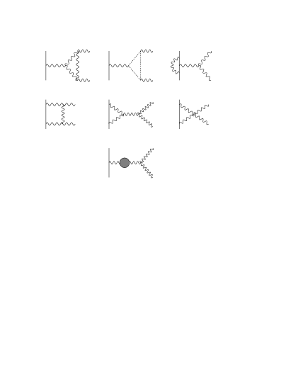
Figure 3: Diagrams contributing to ${\cal T}^{ab}_{1\mu\nu}$. The blob refers to the same corrections to the gluon propagator as in Fig.2(a,e,f).

Figure 4: Diagrams contributing to ${\cal T}^{abc}_{\mu\nu\rho}$. We do not show the diagrams which are related to those shown by exchange of outgoing bosons.

Proceeding to the two-loop analysis, one must consider two separate quantities: ${\cal A}_{2g}(s,\alpha^{3})$, which is the contribution to the imaginary part of the two-loop amplitude which arises from the convolution of the tree-level amplitude for $q(p_{1})\bar{q}(p_{2})\rightarrow g(k_{1})g(k_{2})$ with the hermitian conjugate of its one-loop partner, see Fig.3, and ${\cal A}_{3g}(s,\alpha^{3})$, which is the contribution to the imaginary part which arises on convoluting the tree-level amplitude for the process $q(p_{1})\bar{q}(p_{2})\rightarrow g(k_{1})g(k_{2})g(k_{3})$ with its hermitian conjugate, see Fig.4. The two contributions must then be fed into a twice-subtracted dispersion relation and integrated from $4M^{2}$ to $\infty$ and from $9M^{2}$ to $\infty$ respectively, i.e.

$$\Re{\rm e}\ \widehat{\Pi}(s,\alpha^{2}))=\frac{(s-M^{2})^{2}}{\pi}\Bigg{[}\int\limits^{\infty}_{4M^{2}}\,\frac{ds^{\prime}\,\Im{\rm m}\ \widehat{\Pi}_{2g}(s^{\prime},\alpha^{2})}{(s^{\prime}-M^{2})^{2}(s^{\prime}-s)}\,+\int\limits^{\infty}_{9M^{2}}\,\frac{ds^{\prime}\,\Im{\rm m}\ \widehat{\Pi}_{3g}(s^{\prime},\alpha^{2})}{(s^{\prime}-M^{2})^{2}(s^{\prime}-s)}\Bigg{]}$$ (5.5)

where

$${\cal A}_{ng}(s,\alpha^{3})=2D_{0}(s)\ V_{\mu c}V^{\mu}_{c}\ \Im{\rm m}\ \widehat{\Pi}_{ng}(s,\alpha^{2}).$$ (5.6)

If our calculations reveal that the RHS of (5.5) is infinite then we will have shown that the $S$-matrix element for $q\bar{q}\to q\bar{q}$ computed in the framework of the MYM is not renormalisable at two loops.

We shall now show that ${\cal A}_{2g}$, when fed into the integral on the RHS of (5.5), gives a finite contribution, wheras the ${\cal A}_{3g}$ integral needs an additional subtraction in order to be rendered finite, i.e. it gives rise to a non-renormalisable contribution.

To see that the contribution from ${\cal A}_{2g}$ contains no dangerous terms, it suffices to prove that (a) the one-loop amplitude ${\cal T}_{1\mu\nu}^{ab}$ for $q\bar{q}\to gg$ is renormalisable, and (b) that it satisfies exactly the same type of BRST identity as its tree-level counterpart ${\cal T}_{0\mu\nu}^{ab}$, i.e. that (5.1) holds if we replace ${\cal T}_{0\mu\nu}^{ab}\rightarrow{\cal T}_{1\mu\nu}^{ab}$ and ${\cal S}_{0}^{ab}\rightarrow{\cal S}_{1}^{ab}$. Both (a) and (b) can be easily proved based on the analysis of [28]. It turns out that the closed expressions for ${\cal T}_{1\mu\nu}^{ab}$ and ${\cal S}_{1}^{ab}$ are given by the Feynman diagrams of regular QCD in the Feynman gauge, but with the tree-level propagators inside all graphs replaced by massive ones, again in the Feynman gauge, with the exception that for the ghost contributions we have a different statistical factor. This discrepancy does not affect the high energy behaviour of such graphs, i.e. the ghost loops are well-behaved for large $q^{2}$. In addition, as follows from [28], the tree-level BRST identities do indeed hold at one loop. Thus

$${\cal A}_{2g}(s,\alpha^{3}) = \frac{1}{2}\,\int 2\ \Re{\rm e}[{\cal T}_{1\mu\nu}\,Q^{\mu\rho}(k_{1})\,Q^{\nu\sigma}(k_{2})\,{\cal T}_{0\rho\sigma}^{\dagger}]d(P.S.{}^{2})$$ (5.7)

$$= \frac{1}{2}\,\int 2\ \Re{\rm e}[\Big{(}{\cal T}_{1}^{\mu\nu}{\cal T}_{0\mu\nu}^{\dagger}\ -\ {\cal S}_{1}{\cal S}_{0}^{\dagger}\Big{)}]d(P.S.{}^{2})$$

and the real part can be obtained using the twice-subtracted dispersion relation.

Now we turn to the amplitude ${\cal T}_{\mu\nu\rho}^{abc}(k_{1},k_{2},k_{3})$ for the process $q(p_{1})\bar{q}(p_{2})\rightarrow g(k_{1})g(k_{2})g(k_{3})$, where $k_{i}$ is the four-momentum of the $i$-th gluon, and $p_{1}+p_{2}=q=k_{1}+k_{2}+k_{3}$. Such an amplitude is given by the sum of the diagrams shown in Fig.4

Let us compute the quantity

$${\cal A}_{3g}(s,\alpha^{3})=\frac{1}{3!}\int[{\cal T}_{\mu\nu\rho}\,Q^{\mu\sigma}(k_{1})\,\,Q^{\nu\lambda}(k_{2})Q^{\rho\tau}(k_{3})\,{\cal T}_{\sigma\lambda\tau}^{\dagger}]d(P.S.{}^{3})$$ (5.8)

where $\int d(P.S.{}^{3})$ denotes the integration over the three-body phase space, with the combinatorial factor $1/3!$ accounting for the three indistinguishable gluons in the final state. As before, the polarisation tensors satisfy the transversality condition: $k_{i}\cdot Q(k_{i})=0$. At first sight, the integrand in (5.8) seems to contain terms proportional to $(M^{-2})^{0}$, $(M^{-2})^{1}$, $(M^{-2})^{2}$ and $(M^{-2})^{3}$. The term proportional to $(M^{-2})^{0}$ is renormalisable, whereas all higher powers give rise to non-renormalisable contributions: The higher the power, the worse the divergence. However, as we shall shortly see, by virtue of the BRST identities that ${\cal T}_{\mu\nu\rho}$ satisfies and the transversality properties of the polarisation tensors, only terms proportional to $(M^{-2})^{0}$ and $(M^{-2})^{1}$ survive. Thus, the worst divergence is logarithmic.

To establish this fact, let us first study the action of the longitudinal momenta $k_{1}^{\mu}$, $k_{2}^{\nu}$, and $k_{3}^{\rho}$ on ${\cal T}_{\mu\nu\rho}$. It is straightforward to verify that ${\cal T}_{\mu\nu\rho}^{abc}(k_{1},k_{2},k_{3})$ satisfies the following identities:

$$k^{\mu}_{1}{\cal T}_{\mu\nu\rho}^{abc} = ({\cal S}_{12})_{\rho}^{abc}k_{2\nu}+({\cal S}_{13})_{\nu}^{abc}k_{3\rho}\,,$$

$$k^{\nu}_{2}{\cal T}_{\mu\nu\rho}^{abc} = ({\cal S}_{21})_{\rho}^{abc}k_{1\mu}+({\cal S}_{23})_{\mu}^{abc}k_{3\rho}\,,$$

$$k^{\rho}_{3}{\cal T}_{\mu\nu\rho}^{abc} = ({\cal S}_{31})_{\nu}^{abc}k_{1\mu}+({\cal S}_{32})_{\mu}^{abc}k_{2\nu}\ .$$ (5.9)

Bose symmetry imposes the following relations among the $S_{ij}$ amplitudes:

$${\cal S}_{ij}^{a_{i}a_{j}a_{\ell}}(k_{i},k_{j},k_{\ell}) = {\cal S}_{ji}^{a_{j}a_{i}a_{\ell}}(k_{j},k_{i},k_{\ell})$$

$${\cal S}_{ij}^{a_{i}a_{j}a_{\ell}}(k_{i},k_{j},k_{\ell}) = {\cal S}_{i\ell}^{a_{i}a_{\ell}a_{j}}(k_{i},k_{\ell},k_{j})$$ (5.10)

and

$$k_{i}\cdot{{\cal S}}_{jl}=k_{j}\cdot{{\cal S}}_{il}~{},~{}~{}~{}l\neq i\neq j.$$ (5.11)

The closed form of ${\cal S}_{23}^{abc}(k_{1},k_{2},k_{3})$ reads

$$({\cal S}_{23})^{abc}_{\mu}=({\cal S}^{s}_{23})^{abc}_{\mu}+({\cal S}^{t}_{23})^{abc}_{\mu}$$ (5.12)

with

$$({\cal S}^{s}_{23})^{abc}_{\mu} = g^{2}V_{e}^{\alpha}\Bigg{[}f^{elc}f^{lab}\frac{k_{3}^{\sigma}\Gamma_{\alpha\sigma\mu}(q,k_{1}-q,-k_{1})}{2k_{2}\cdot k_{3}+M^{2}}+f^{eal}f^{lbc}\frac{k_{3\alpha}(k_{1}+k_{2})_{\mu}}{2k_{1}\cdot k_{2}+M^{2}}+f^{elb}f^{lac}\frac{k_{2\alpha}k_{3\mu}}{2k_{1}\cdot k_{3}+M^{2}}\Bigg{]}$$

$$({\cal S}^{t}_{23})^{abc}_{\mu} = -ig^{2}\bar{v}(p_{2})\left(\,T^{a}\gamma_{\mu}\,\frac{1}{\not\!k_{1}-\not\!p_{2}}\,T^{e}\gamma_{\sigma}+T^{e}\gamma_{\sigma}\,\frac{1}{\not\!p_{1}-\not\!k_{1}}\,\gamma_{\mu}T^{a}\,\right)u(p_{1})\frac{f^{eac}k_{1}^{\sigma}}{2k_{2}\cdot k_{3}+M^{2}}.$$

In deriving the above expressions, in addition to the elementary Ward identity, (3.9), we have employed the tree-level Ward identity:

$$q^{\mu}_{1}\Gamma_{\mu\nu\alpha\beta}^{abcd}(q_{1},q_{2},q_{3},q_{4})= f^{abe}\Gamma_{\alpha\beta\nu}^{cde}(q_{3},q_{4},q_{1}+q_{2})+f^{ace}\Gamma_{\beta\nu\alpha}^{dbe}(q_{4},q_{2},q_{1}+q_{3})$$ (5.14)

$$+f^{ade}\Gamma_{\nu\alpha\beta}^{bce}(q_{2},q_{3},q_{1}+q_{4}),$$

which relates the bare three- and four-gluon vertices. All remaining $S_{ij}$ amplitudes can be obtained from $S_{12}$ using the relations of (5.10).

We next let the longitudinal momenta in the polarisation tensors act on ${\cal T}_{\mu\nu\rho}$ and ${\cal T}_{\sigma\lambda\tau}$, and use (5.9). We can see how the $(M^{-2})^{3}$ terms disappear. The action of the term $M^{-2}k_{3}^{\rho}k_{3}^{\tau}$ gives terms proportional to $k_{1}^{\mu}$ and $k_{2}^{\nu}$ (or equivalently $k_{1}^{\sigma}$ and $k_{2}^{\lambda}$), which vanish when they hit $Q^{\mu\sigma}(k_{1})$ or $Q^{\nu\lambda}(k_{2})$. So, (5.8) reduces to

$${\cal A}_{3g}=\frac{1}{3!}\int\Bigg{[}{\cal T}_{\mu\nu\rho}Q^{\mu\sigma}(k_{1})\,Q^{\nu\lambda}(k_{2})\,{\cal T}_{\sigma\lambda\rho}^{\dagger}\Bigg{]}d(P.S.{}^{3}).$$ (5.15)

At this point, the highest possible power of $M^{-2}$ is $(M^{-2})^{2}$ . We now let $M^{-2}k_{2}^{\nu}k_{2}^{\lambda}$ act on ${\cal T}_{\mu\nu\rho}$ and ${\cal T}_{\sigma\lambda\rho}^{\dagger}$:

$$M^{-2}k_{2}^{\nu}k_{2}^{\lambda}{\cal T}_{\mu\nu\rho}\,Q^{\mu\sigma}(k_{1})\,{\cal T}_{\sigma\lambda\rho}^{\dagger} = ({\cal S}_{21}^{\rho}k_{1}^{\mu}+{\cal S}_{23}^{\mu}k_{3}^{\rho})\,Q_{\mu\sigma}(k_{1})\,({\cal S}_{21\rho}k_{1}^{\sigma}+{\cal S}_{23}^{\sigma}k_{3\rho})^{\dagger}$$ (5.16)

$$= {\cal S}_{23}^{\mu}{\cal S}_{23}^{\sigma\dagger}\,Q_{\mu\sigma}(k_{1}).$$

Thus, one more power of $M^{-2}$ has been eliminated. We are left with

$${\cal A}_{3g} = \frac{1}{3!}\int[({\cal T}_{\mu\nu\rho}{\cal T}_{\sigma\nu\rho}^{\dagger}-{\cal S}_{23}^{\mu}{\cal S}_{23}^{\dagger\sigma})\,Q^{\mu\sigma}(k_{1})]d(P.S.{}^{3}),$$ (5.17)

$$= {\cal A}_{R}+{\cal A}_{NR},$$

where

$${\cal A}_{3g}^{R}=\frac{1}{3!}\int[{\cal T}_{\mu\nu\rho}{\cal T}_{\mu\nu\rho}^{\dagger}-3({\cal S}_{12}{\cal S}_{12}^{\dagger})]d(P.S.{}^{3}),$$ (5.18)

$${\cal A}_{3g}^{NR}=-\frac{1}{3!}\frac{1}{M^{2}}\int(k_{1}\cdot{\cal S}_{23})(k_{1}\cdot{\cal S}_{23})^{\dagger}d(P.S.{}^{3}).$$ (5.19)

In deriving the above expressions we have used the fact that the phase-space integration is invariant under $k_{i}\leftrightarrow k_{j}$. The term in (5.19) will generate non-renormalisable terms; it is clearly non-vanishing, since it is a three-body phase-space integral over a positive definite quantity. In particular,

$${\cal A}_{3g}^{NR}=-\frac{1}{3!}\frac{c_{A}^{2}}{8M^{2}}\int V^{e}_{\alpha}(k_{1}-k_{2})^{\alpha}(k_{1}-k_{2})^{\beta}V^{e}_{\beta}d(P.S.{}^{3})$$ (5.20)

where the identities $f^{abe}f^{cde}+f^{ace}f^{dbe}+f^{ade}f^{bce}=0$ and $f^{alm}f^{bmn}f^{cnl}=\frac{1}{2}c_{A}f^{abc}$ have been used. We also used $\frac{k_{i}\cdot k_{j}}{2k_{i}k_{j}+M^{2}}=\frac{1}{2}+...$, where the omitted term is proportional to $M^{2}$, thus giving rise to a renormalisable contribution, i.e. the omitted term belongs effectively to ${\cal A}_{3g}^{R}$. Notice that the non-renormalisable terms are purely propagator-like (universal, process-independent).

Finally, it is instructive to compare the result of (5.17) with that of normal QCD. In the QCD case there are, of course, no terms proportional to $M^{-2}$ or higher powers. On the other hand, the presence of the auxiliary four-vector $\eta_{\mu}$ in the polarisation tensors could in principle induce spurious divergences, should it survive in the final answer. It is easy to see however how any reference to $\eta_{\mu}$ disappears before any of the phase-space integrations are carried out. Let us denote the corresponding QCD amplitude by ${\widehat{\cal T}}_{\mu\nu\rho}$. We start again with

$${\cal A}_{3g}^{QCD}=\frac{1}{3!}\int[{\widehat{\cal T}}_{\mu\nu\rho}\,\,P^{\mu\sigma}(k_{1})\,\,P^{\nu\lambda}(k_{2})\,P^{\rho\tau}(k_{3})\,{\widehat{\cal T}}_{\sigma\lambda\tau}^{\dagger}]d(P.S.{}^{3})$$ (5.21)

where the gluons are now massless and $k_{i}\cdot P(k_{i})=0$  $(i=1,2,3)$. Equation (5.9) is valid for QCD, as can be shown rigorously using BRST arguments. Since the elementary Ward identity (3.9) is the same for both MYM and massless QCD, it follows that the closed expressions for the factors $S_{ij}$ in (5.9) may be recovered from (LABEL:S23) simply by setting $M^{2}=0$. We denote them by ${\widehat{S}}_{ij}$. Then, by letting the longitudinal momenta act on ${\widehat{\cal T}}_{\mu\nu\rho}$ and using (5.9), one can easily verify that any reference to the four-vector $\eta_{\mu}$ disappears and that the final answer is

$${\cal A}_{3g}^{QCD}=\frac{1}{3!}\int[{\widehat{\cal T}}^{\mu\nu\rho}{\widehat{\cal T}}_{\mu\nu\rho}^{\dagger}-6{\widehat{{\cal S}}}_{12}{\widehat{{\cal S}}}_{12}^{\dagger}]d(P.S.{}^{3}).$$ (5.22)

So, unlike the MYM model, in massless QCD all potentially dangerous terms vanish.

6 Connection to field theories with a Higgs mechanism

It is well known that the only way to endow gauge fields with mass whilst maintaining unitarity and renormalisability is via the Higgs mechanism [19, 20, 21]. This procedure is not suitable however for an effective model of strong interactions because it introduces extra scalar particles in the physical spectrum. In the MYM model massive gauge fields are obtained without introducing extra physical fields, at the price of losing renormalisability at higher orders of perturbation theory. It is instructive to see explicitly how the lack of renormalisability in the MYM can be traced back to the absence of a Higgs particle; in particular understand why the process $q\bar{q}\to q\bar{q}$ (and $q\bar{q}\to gg$) is renormalisable at one-loop, but ceases to be renormalisable beyond one-loop. In this section we address these issues in detail by performing a quantitative analysis of the differences and similarities between the MYM and a Higgs model (HM) at the level of the $S$-matrix. In addition, as has been discussed in detail in [16], it is possible to speak about the MYM using the language of a HM. Specifically, one can think of the MYM as a theory where all gluons have been given masses by adding to the Lagrangian a sufficient number of Higgs multiplets ($N$ fundamental representations of $SU(N)$ ), and then “freezing” all the polar excitations of the $N$ Higgs fields. The remaining $N^{2}-1$ angular excitations corresponding to the Goldstone bosons are precisely the angular fields $\theta^{a}$ displayed in (2.10).

To illustrate the above points we will use a toy Higgs field theory which displays all the essential features we want to study. The gauge group of this model is SU(2). The Higgs mechanism is triggered by a complex doublet $\phi$ in the fundamental representation (isospin $l=\frac{1}{2}$). This particular assignment endows all three gauge bosons with the same mass $M$, whilst simultaneously prohibiting terms of the form ${\phi}\bar{\psi}{\psi}$ for any fermion representation of isospin $\ell$ . To mimic QCD, we choose the fundamental representation for the massless fermion fields $\psi$, although this choice is not essential for what follows. As there are no interactions between fermions and scalars, the fermions remain massless even when the scalar fields acquire a non-vanishing vacuum expectation value. The Lagrangian density for this model is

$${\cal L}=-\frac{1}{4}{\cal F}_{\mu\nu}{\cal F}^{\mu\nu}+\bar{\psi}{\not\!D}{\psi}+({D}_{\mu}{\phi})({D}^{\mu}{\phi})^{\dagger}-V({\phi})$$ (6.1)

with

$$({\not\!D}{\psi})_{\alpha} = {\not\!\partial}{\psi}_{\alpha}+igT^{a}_{\alpha\beta}{\psi}_{\beta}{\not\!A}^{a}~{},$$

$$(D_{\mu}{\phi})^{i} = \partial_{\mu}{\phi}^{i}+ig{T}^{ij}_{a}{\phi}_{j}A^{a}_{\mu}~{},$$

$$V(\phi) = {\mu}^{2}{\phi}{\phi}^{\dagger}+\lambda({\phi}{\phi}^{\dagger})^{2},$$ (6.2)

where ${T}_{a}=\frac{1}{2}{\sigma}_{a}$, and ${\sigma}_{a}$ are the Pauli matrices. If ${\mu}^{2}<0$, the Higgs mechanism gives rise to three degenerate massive gauge bosons of mass $M=gv/2$, where $v=\sqrt{-\frac{\mu^{2}}{\lambda}}$ is the minimum of $V(\phi)$. The above model is a vector-like variant of the usual electroweak sector of the Standard Model, $SU(2)\times U(1)$, with the Weinberg angle $\theta_{W}$ set to zero.

The corresponding bare gauge boson propagator in the $R_{\xi}$ gauge has the form

$$\Delta_{\mu\nu}=\Bigg{(}g_{\mu\nu}-\frac{q_{\mu}q_{\nu}(1-\xi)}{q^{2}-{\xi}M^{2}}\Bigg{)}\frac{-i}{q^{2}-M^{2}}$$ (6.3)

and the would-be Goldstone boson ($G$) and ghost ($c$) propagators are

$$\Delta_{G,c}=\frac{i}{q^{2}-{\xi}M^{2}}.$$ (6.4)

In the unitary gauge, which formally corresponds to the limit $\xi\rightarrow\infty$, the gauge boson propagator takes the form (4.32) and there are no Goldstone boson/ghost propagators. Finally, there is a Higgs particle of mass $M_{H}=v\sqrt{2\lambda}$ with bare propagator

$$\Delta_{H}=\frac{i}{q^{2}-M_{H}^{2}}~{}.$$ (6.5)

The one-loop $\beta$-function for the gauge coupling has the form [30]

$$\beta=-\frac{1}{16{\pi}^{2}}(b_{g}-b_{f}-b_{s})g^{3}$$ (6.6)

with

$$b_{g}=\frac{11}{3}c_{A}~{},~{}~{}~{}b_{f}=\frac{4}{3}n_{f}T_{f}~{},~{}~{}~{}b_{s}=\frac{1}{6}n_{s}T_{s}~{},$$ (6.7)

where $T_{f}$ is the Dynkin index of the fermion representation, $T_{s}$ is the Dynkin index of the scalar representation, $n_{f}$ is the number of fermion families in a given representation and $n_{s}$ the number of real scalar families. For the particular scalar representation we have chosen, $T_{s}=\frac{1}{2}$ and $n_{s}=2$. In the absence of quarks we have that $\beta=-\frac{g^{3}}{16{\pi}^{2}}(43/6)$.

Figure 5: Higgs boson contributions to $\widehat{\Pi}_{\mu\nu}^{gH}$. In the unitary gauge recall that (b) is absent.

Let us now proceed with a study of the one-loop amplitude. As we already showed, at the level of $S$-matrix elements the MYM and the naive model are equivalent. In addition, if we adopt the unitary gauge for the HM then it is obvious that, to any finite order in perturbation theory, the only difference between an $S$-matrix element computed in the MYM and the corresponding $S$-matrix element computed in the HM is due to contributions to the latter which come from Feynman diagrams containing Higgs boson propagators [31]. For example, in the case of one-loop quark scattering, in addition to the graphs in Fig.2, which are common to both MYM and HM, the diagram of Fig.5(a) contributes to the $S$-matrix element of the HM. In other words, the $S$-matrix elements of the MYM model may be obtained from the corresponding $S$-matrix elements of HM by omitting all diagrams containing a Higgs particle. Given this observation, it is easy to see why the the process $qq\to qq$ in the MYM is renormalisable at one loop: The only difference between the renormalisable HM and the MYM is the contribution corresponding to the graphs of Fig.5, which themselves form a gauge-invariant and renormalisable subset. Denoting their contribution by $\widehat{\Pi}_{\mu\nu}^{gH}$ we have that, up to the immaterial tadpole graph,

$$\widehat{\Pi}_{\mu\nu}^{gH}=g^{2}M^{2}\int\frac{d^{n}k}{i(2\pi)^{n}}\left(-g_{\mu\nu}+\frac{k_{\mu}k_{\nu}}{M^{2}}\right)\frac{1}{(k^{2}-M^{2})[(k+q)^{2}-M_{H}^{2}]}.$$ (6.8)

The factor $M^{2}$ in front of the integral originates from the gluon-gluon-Higgs coupling and guarantees that $\widehat{\Pi}_{\mu\nu}^{gH}$ can be made ultraviolet-finite by means of the usual mass and wave function renormalisation. After (on-shell) renormalisation, the above expression becomes, in the limit $q^{2}\gg M^{2}$, (and dropping the terms proportional to $q^{\mu}q^{\nu}$)

$$\widehat{\Pi}_{\mu\nu}^{gH}(q^{2})=-\frac{\alpha}{4\pi}\left(\frac{1}{12}\right)q^{2}\ln(q^{2}/M^{2})g^{\mu\nu}+...$$ (6.9)

where the ellipsis denotes numerical constants and terms of order $O(M^{2}/q^{2})$. If we now set $c_{A}=2$ in the expression of (4.27), and add it to the expression in (6.9), we see that the coefficient in front of the resulting logarithmic term is equal to $43/6$, which is precisely the coefficient of the HM $\beta$-function without quarks. In addition, as expected from the discussion on the connection between the MYM and the HM given at the beginning of this section, the expression in (6.9) is exactly the difference between (4.27) and (4.28) for $c_{A}=2$.

Figure 6: The Higgs graphs contributing to ${\cal T}_{1}^{H}$. The graphs of Fig.3 must also be included when computing ${\cal T}_{1}^{H}$.

We now turn to the two-loop analysis. Firstly, it is relatively straightforward to establish that the contribution from the two-gluon cut of those one-loop diagrams which contain a Higgs boson, Fig.6, gives rise to a renormalisable contribution, i.e. the corresponding dispersive (real) part can be made finite by means of a twice-subtracted dispersion relation. This is of course expected, since the one-loop diagrams contributing to ${\cal A}_{2g}$ which we studied in the previous section were themselves renormalisable, i.e. no cancellation from diagrams containing a Higgs boson is required.

To see this explicitly, consider the amplitude ${\cal A}_{2g}^{H}$ given by

$${\cal A}_{2g}^{H}(s)=\frac{1}{2}\,\int 2\ \Re{\rm e}[{\cal T}_{1\mu\nu}^{H}\,Q^{\mu\rho}(k_{1})\,Q^{\nu\sigma}(k_{2})\,{\cal T}_{0\rho\sigma}^{\dagger}]d(P.S.{}^{2})$$ (6.10)

where ${\cal T}_{1\mu\nu}^{H}$ is shown in Fig.6. It is straightforward to verify that ${\cal T}_{1\mu\nu}^{H}$ is a gauge-independent quantity, and that it satisfies

$$k^{\mu}_{1}{\cal T}_{1\mu\nu}^{H}=k_{2\nu}{\cal S}_{1}^{H}$$ (6.11)

with

$${\cal S}_{1}^{H}=gV^{\lambda}D^{0}(q)[\widehat{\Pi}^{gH}_{\lambda\alpha}D^{0}(q)](k_{1}-k_{2})^{\alpha}.$$ (6.12)

Notice that the expression in square brackets behaves like $\log(s/M^{2})$ for $s\gg M^{2}$. Using (5.1) and (6.11) we can see that

$${\cal A}_{2g}^{H}(s)=\frac{1}{2}\,\int 2\Re{\rm e}[\Big{(}{\cal T}_{1\mu\nu}^{H}{\cal T}_{0}^{\mu\nu\dagger}\ -\ {\cal S}_{1}^{H}{\cal S}_{0}^{\dagger}\Big{)}]d(P.S.{}^{2}).$$ (6.13)

So, this contribution gives rise to renormalisable two-loop amplitudes.

Figure 7: One of the graphs contributing to ${\cal T}_{\mu\nu\rho}^{H}$. The others are obtained by permuting the outgoing bosons.

To see how the presence of the Higgs boson enforces renormalisability, we focus on the two amplitudes, ${\cal A}_{3g}^{H,a}$ and ${\cal A}_{3g}^{H,b}$:

$${\cal A}_{3g}^{H,a}(s)=\frac{1}{3!}\int[{\cal T}_{\mu\nu\rho}^{H}\,Q^{\mu\sigma}(k_{1})\,\,Q^{\nu\lambda}(k_{2})Q^{\rho\tau}(k_{3})\,{\cal T}_{\sigma\lambda\tau}^{H\dagger}]d(P.S.{}^{3})$$ (6.14)

and

$${\cal A}_{3g}^{H,b}=\frac{1}{3!}\int 2\Re{\rm e}[{\cal T}_{\mu\nu\rho}^{H}\,Q^{\mu\sigma}(k_{1})\,\,Q^{\nu\lambda}(k_{2})Q^{\rho\tau}(k_{3})\,{\cal T}_{\sigma\lambda\tau}^{\dagger}]d(P.S.{}^{3})$$ (6.15)

where the amplitude ${\cal T}_{\mu\nu\rho}^{H}$ is shown in Fig.7. As can be seen, ${\cal A}_{3g}^{H,a}$ arises by multiplying only those three-gluon amplitudes which contain Higgs particles whilst ${\cal A}_{3g}^{H,b}$ comes from interfering the Higgs diagrams with the non-Higgs diagrams of Fig.4. Since the coupling of the Higgs boson to two gauge bosons is proportional to $M$, it follows that ${\cal T}_{\mu\nu\rho}^{H}$ has already a factor $M^{2}$ built into it. Consequently, there is an implicit factor $M^{4}$ inside ${\cal A}_{3g}^{H,a}(s)$, and therefore the only non-renormalisable contribution in ${\cal A}_{3g}^{H,a}(s)$ will come from the term in the polarisation tensors which is proportional to $(M^{-2})^{3}$. We therefore find that

$$[{\cal A}_{3g}^{H,a}]_{NR}(s)=-(\frac{1}{2})\frac{1}{3!}\frac{1}{M^{2}}\int V^{e}_{\alpha}(k_{1}-k_{2})^{\alpha}(k_{1}-k_{2})^{\beta}V^{e}_{\beta}d(P.S.{}^{3}).$$ (6.16)

The interference term, ${\cal A}_{3g}^{H,b}$, has an implicit $M^{2}$ inside so now contributions from the $(M^{-2})^{3}$ and $(M^{-2})^{2}$ terms in the polarisation tensors are needed. One finds, using (5.9), the following non-renormalisable contribution:

$$[{\cal A}_{3g}^{H,b}]_{NR}(s)=\frac{1}{3!}\frac{1}{M^{2}}\int V^{e}_{\alpha}(k_{1}-k_{2})^{\alpha}(k_{1}-k_{2})^{\beta}V^{e}_{\beta}d(P.S.{}^{3}).$$ (6.17)

In arriving at the above results, identities of the type $k_{1}^{\alpha}k_{1}^{\beta}=\frac{1}{3}(k_{1}-k_{2})^{\alpha}(k_{1}-k_{2})^{\beta}$, or $k_{2}^{\alpha}k_{3}^{\beta}=-\frac{1}{2}k_{3}^{\alpha}k_{3}^{\beta}$ valid under the integral sign, may be found useful. Comparing to (5.20) of the previous section (setting $c_{A}=2$), we see that the Higgs contribution exactly cancels the non-renormalisable part of the MYM two-loop contribution. Evidently, even though the Higgs boson does not couple directly to the quarks, (since in this toy model the gauge symmetry prohibits Yukawa couplings) its importance in restoring the renormalisability of the process $q\bar{q}\to q\bar{q}$ manifests itself through the tree-level sub-amplitudes $gg\to gg$ containing the Higgs boson (Fig.7), which reside in the two-loop diagrams.

7 Quark-Quark Elastic Scattering

In this section we take an introductory look at the elastic scattering of a pair of quarks via two-gluon exchange within the MYM model. Of course, quark-quark elastic scattering cannot be measured directly, but it is possible that many of the elements which are central to the more realistic processes (e.g. hadron-hadron elastic scattering) are contained in this simpler treatment. This is in the spirit of the Donnachie-Landshoff-Nachtmann approach [3, 32], where the success of the additive quark rule provides evidence that one need not know about the detailed structure of the colliding hadrons before one can proceed to make elastic scattering calculations, although it is not yet established that this is correct [33].

As a first step, one can calculate the amplitude for the elastic scattering of differently flavoured quarks, i.e. $q_{i}q_{j}\to q_{i}q_{j}$, at the lowest order, keeping only those terms which dominate in the Regge limit. This is a straightforward calculation of the box diagram shown in Fig.2(c) rotated through 90 degrees (the crossed box diagram contributes only to the real part of the amplitude in the Regge limit and constitutes a sub-leading correction). The leading contribution is imaginary and so can be obtained directly using the cutting rules, i.e. the amplitude for single gluon exchange can be written:

$$A(s,t)_{1-{\rm gluon}}=iT^{a}\otimes T^{a}2p_{1}^{\mu}\frac{g_{\mu\nu}}{k^{2}-M^{2}}2p_{2}^{\nu}\delta_{\lambda_{1}\lambda_{1}^{\prime}}\delta_{\lambda_{2}\lambda_{2}^{\prime}},$$ (7.18)

where $k$ is the momentum of the exchanged gluon and $p_{1}$ and $p_{2}$ are the momenta of the incoming quarks, i.e. $s=(p_{1}+p_{2})^{2}$. The high-energy limit allows the exchanged gluon to be assumed soft, and so the eikonal approximation has been used to simplify the $qqg$ vertex. The delta functions ensure helicity conservation at each vertex. Multiplying by the conjugate amplitude, projecting out the colour singlet part and performing the two-body phase space integral (putting the intermediate quarks on-shell) allows us to write

$$A(s,t)=is\alpha_{s}^{2}\frac{N^{2}-1}{N^{2}}\int d^{2}{\bf k}\frac{1}{({\bf k}^{2}+M^{2})(({\bf k-q})^{2}+M^{2})},$$ (7.19)

where ${\bf q}^{2}=-t>0$, $N$ is the number of colours and the exchanged gluons are taken to be purely transverse. The transverse momentum integral can be performed and yields

$$A(s,t)=i\frac{s}{-t}2\pi\alpha_{s}^{2}\frac{N^{2}-1}{N^{2}}\frac{1}{\Delta(t)}\ln\frac{\Delta(t)+1}{\Delta(t)-1},$$ (7.20)

where $\Delta(t)$ is defined in (3.28). Thus, the total cross-section for $q_{i}q_{j}\to X$ is

$$\sigma_{T}=\frac{1}{M^{2}}\pi\alpha_{s}^{2}\frac{N^{2}-1}{N^{2}}.$$ (7.21)

It is instructive to investigate the conditions under which the two-gluon exchange amplitude calculated above violates unitarity. We shall see that unitarity is violated only for very central collisions and that these constitute an insignificant fraction of the total and elastic scattering cross-sections. Only for very high-$t$ processes do we have collisions which are sufficiently central to cause a worry. This gives us confidence to proceed to the next order of calculation, assured that we have yet to receive indications that unitarisation corrections are important.

To investigate unitarity we perform a Fourier transform of the elastic scattering amplitude, i.e.

$$\tilde{A}(s,b)=\int\frac{d^{2}{\bf q}}{(2\pi)^{2}}e^{-i{\bf q}\cdot{\bf b}}\frac{A(s,t)}{2s},$$ (7.22)

and ${\bf b}$ is the impact parameter of the collision. Written in this way, unitarity demands that

$$|\tilde{A}(s,b)|^{2}<1$$

for all ${\bf b}$. However, we can be confident that unitarisation corrections are small if the inequality is satisfied for those values of impact parameter which dominate the process under study. Numerical evaluation of (7.22) demonstrates that the amplitude only ever violates unitarity for $Mb<10^{-2}$, $10^{-3}$ for $2/\alpha_{s}^{2}=20$, $50$ respectively, i.e. only for very central collisions (on the scale of the gluon mass). In this language, the total cross-section is given by

$$\sigma_{T}=2\int d^{2}{\bf b}\ \tilde{A}(s,b)$$ (7.23)

whilst the elastic scattering cross-section is given by

$$\sigma_{{\rm el}}=\int d^{2}{\bf b}\ |\tilde{A}(s,b)|^{2}.$$ (7.24)

Since $\tilde{A}(s,b)$ decreases monotonically as $Mb$ increases, it follows that the elastic scattering cross-section receives a larger contribution from more central collisions than the total cross-section. To a first approximation, the typical impact parameter is set by the gluon mass, i.e. $\langle b^{2}\rangle=C/M^{2}$ where $C\sim 1$ and is larger for the total cross-section than for the elastic cross-section. In either case, we are always well away from the dangerous region where unitarity is violated. The situation is different for high-$t$ processes, since now $\langle b^{2}\rangle\sim 1/|t|$ and so, for $\sqrt{-t}>(10^{2}-10^{3})M$ we would need to worry that unitarisation corrections are important.

8 Conclusion and Perspectives

In this paper we have reviewed and investigated the formalism of the MYM model, arguing that it may be relevant as a tool to investigate diffractive scattering (and possibly other areas of strong interactions phenomenology), where traditional QCD methods are inadequate. A detailed study of the $q\bar{q}\to q\bar{q}$ process in the context of this model up to the two-loop order was presented, and the renormalisation properties of the corresponding $S$-matrix were discussed.

Let us summarise briefly the prospects for a study of diffractive scattering. A successful model of diffraction should be able to explain: The growth of total hadronic cross-sections with increasing $s$. In particular, the model should show why the rise in soft hadronic processes (e.g. the total $pp$ cross-section) proceeds at a much slower rate than in hard processes (e.g. the $\gamma^{*}p$ cross-section); the shrinkage of the forward diffraction peak with increasing $s$. In other words, the model should be able to explain the qualitative success of the Donnachie-Landshoff-Nachtmann model of the pomeron as a single Regge pole in soft diffraction (i.e. in those processes where there is no large scale) and its failure in small-$x$ deep inelastic scattering, in the diffractive production of all vector mesons at high $Q^{2}$ and in the diffractive production of $J/\Psi$ mesons at low $Q^{2}$.

In the future, we plan to use the MYM model to compute the complete ${\cal O}(\alpha_{s})$ corrections to the two-gluon-exchange amplitude discussed in the previous section, in order to verify whether some or all of the aforementioned features emerge. More specifically, such a calculation should help us investigate the following points:

• In the limit of large enough $s$, the logarithms $\sim(\alpha_{s}\ln s)^{m}$, which appear at each order in perturbation theory, become large and it becomes necessary to sum them to all orders. This summation of leading logarithms is performed using the formalism of BFKL. It is an open question as to precisely when this summation leads to the dominant contribution to the amplitude. In fact, since the summation is of leading logarithms only, we cannot define exactly what it means to say $s$ is large, although we note that, in this respect, analysis of the next-to-leading logarithmic corrections calculated by Fadin, Lipatov et al. [34] should improve the situation. By computing at fixed order in $\alpha_{s}$ we can investigate the relative importance of the $\sim\alpha_{s}\ln s$ term compared to the terms which do not include the logarithm. In this way, we can make some quantitative statements regarding the need (within the MYM model) to sum the remaining leading logarithms. For example, it might be that, at the energies of contemporary colliders, the logarithm is not so large to justify dropping the other terms, i.e. a fixed order calculation might be the better way to proceed.

  It is known that introducing a gluon mass has a very small effect on the leading logarithmic contribution [35, 4]. This arises largely because the BFKL summation is infrared finite, i.e. there are infrared cancellations between real and virtual graphs which reduce the sensitivity to this region. These cancellations persist even after adding a gluon mass (via a Higgs, or via the MYM model) and serve to reduce the sensitivity of the amplitudes to variations in the mass. Note that is not too important how the mass is introduced. This can be seen since no Higgs graphs contribute to the leading logarithm summation and since the gauge-dependent part of the gluon propagator is also sub-leading (in covariant gauges).

• It is also known that the leading logarithm summation leads to a rapid rise of total cross-sections. It can be argued that this rapid rise, which is due to multiple soft gluon emission, reveals itself in hard scattering processes, but is masked in softer processes by unitarity corrections. Any slowing down of the rise via unitarity corrections has yet to be precisely quantified. Another possibility is that the strong rise seen in hard processes can be explained in fixed-order perturbation theory, i.e. arising from the $\ln s$ term, and that this same rise is masked in soft processes by a non-logarithmic contribution which is comparable in size to the logarithmic contribution (i.e. as the process becomes harder, the non-logarithmic contribution falls away to reveal the logarithm). This latter possibility can be investigated after computing the radiative corrections to the two-gluon exchange graphs.

In summary, we think that the MYM may prove a useful tool in understanding the phenomenology of diffractive scattering by bridging the gap between different QCD-inspired models. Such a conjecture will be tested through next-to-leading order calculations of quark-quark elastic scattering, which we plan to discuss in a forthcoming paper.

Acknowledgments We thank V. Del Duca and M. Testa for some useful discussions. This work was supported in part by the EU Fourth Programme ‘Training and Mobility of Researchers’, Network ‘Quantum Chromodynamics and the Deep Structure of Elementary Particles’, contract FMRX-CT98-0194 (DG 12-MIHT). The work of JP is funded by a Marie Curie Fellowship (TMR-ERBFMBICT 972024). JP also acknowledges financial support from the Department of Physics and Astronomy of the University of Manchester while parts of this work were being completed. CP acknowledges the support of PPARC through an Advanced Fellowship.

References

- [1] F.E. Low, Phys. Rev. D12, 163 (1975).
- [2] S. Nussinov, Phys. Rev. Lett. 34, 1286 (1975).
- [3] P.V. Landshoff and O. Nachtmann, Zeit. Phys. C35, 405 (1987).
- [4] V.S. Fadin, E.A. Kuraev, L.N. Lipatov, Sov. Phys. JETP 44, 443 (1976); 45, 199 (1977); Y.Y. Balitsky and L.N. Lipatov, Sov. J. Nucl. Phys. 28, 822 (1978).
- [5] J. M. Cornwall, in Deeper Pathways in High-Energy Physics, edited by B. Kursunoglu, A. Perlmutter, and L. Scott (Plenum, New York, 1977), p 683; Nucl. Phys. B157, 392 (1979).
- [6] R. Jackiw and K. Johnson, Phys. Rev. D8, 2386 (1973); J.M. Cornwall and R. Norton, ibid. D8, 3338 (1973); K. Lane, ibid. D10, 2605 (1974); H. Pagels, ibid. D10, 3080 (1979)
- [7] M. A. Shifman, A. I. Vainstein, and V. I. Zakharov, Nucl. Phys. B147, 385 (1979); B147, 448 (1979).
- [8] J. M. Cornwall, Phys. Rev. D26, 1453 (1982).
- [9] B. Berg, Phys. Lett. B97, 401 (1980); G. Bhanot and C. Rebbi, Nucl. Phys. B189, 469 (1981); C. Bernard, Phys. Lett. B108, 431 (1982); D. B. Leinweber, C. Parrinello, J. I. Skullerud and A. G. Williams, hep-lat/9803015 and references therein.
- [10] V. N. Gribov, Nucl. Phys. B139, 1 (1978); D. Zwanziger, hep-th/9802180 and references therein.
- [11] J. Smit, Phys. Rev. D19, 3013 (1974); R. Fukuda, Phys. Lett. B38, 33 (1978); V. P. Gusynin and V. A. Miransky, ibid B76, 585 (1978); R. Anishetty, M. Baker, S. Kim, J. S. Ball, and F. Zachariasen, ibid. B86, 52 (1979); J. S. Ball, and F. Zachariasen, ibid. 95B, 273 (1980); C. Bernard , Nucl. Phys. B219, 341 (1983); J. F. Donoghue , Phys. Rev. D29, 2559 (1984); F. R. Graziani , Z. Phys. C33, 397, (1987); N. Brown, M.R. Pennington, Phys. Lett. B202, 257 (1988), Erratum-ibid. B205 596, (1988) ; Phys. Rev. D39, 2723 (1989); M. H. Thoma, H. J. Mang, Z. Phys. C44, 349, (1989); E. Bagan , M.R. Pennington , Phys. Lett. B220, 453 (1989); M. Lavelle, Phys. Rev. D44, 26 (1991); J. E. Shrauner, J. Phys. G19, 979 (1993); M. Consoli and J. H. Field, Phys. Rev. D49, 1293 (1994); F.J. Yndurain, Phys. Lett. B345, 524 (1995); I. I. Kogan and A. Kovner, Phys. Rev. D52, 3719 (1995); A. Szczepaniak, E. S. Swanson, C. R. Ji, S. R. Cotanch Phys. Rev. Lett. 76, 2011 (1996).
- [12] P.W. Higgs, Phys. Rev. Lett. 12, 132 (1964); P.W. Higgs, Phys. Rev. 145, 1156 (1966); F. Englert and R. Brout, Phys. Rev. Lett. 13, 321 (1964); G.S. Guralnik, C.R. Hagen, and T.W. Kibble, Phys. Rev. Lett. 13, 585 (1964).
- [13] F. Halzen, G. Krein and A.A. Natale, Phys. Rev. D47, 295 (1993); M.B. Gay Ducati, F. Halzen and A.A. Natale, Phys. Rev. D48, 2324 (1993); J.R. Cudell and B.U. Nguyen, Nucl. Phys. B420, 669 (1994); A. Donnachie and P.V. Landshoff, Phys. Lett. B387, 637 (1996).
- [14] T.Kunimasa and T.Goto, Prog. Theor. Phys. 37, 452 (1967).
- [15] A.A.Slavnov, Theor. Math. Phys. 10, 305 (1972).
- [16] J.M.Cornwall, Phys. Rev. D10, 500 (1974).
- [17] E.C.Stueckelberg, Helv. Phys. Acta. 11, 226 (1938).
- [18] K -I .Shizuya, Nucl. Phys. B87, 255 (1975); ibid. B121, 125 (1977), and references therein.
- [19] J. M. Cornwall, D. N. Levin, and G. Tiktopoulos, Phys. Rev. Lett. 30, 1268 (1973).
- [20] C.H. Llewellyn Smith, Phys. Lett. B46, 233 (1973).
- [21] B.W. Lee, C. Quigg, and H.B. Thacker, Phys. Rev. D16, 1519 (1977).
- [22] S. Weinberg, Phys. Rev. Lett. 27, 1688 (1972); S. Y. Lee, Phys. Rev. D6, 1701 (1972); K. Fujikawa, B. W. Lee, and A. Sanda, ibid. D6, 2923 (1972); T. W. Appelquist and H. R. Quinn, Phys. Lett. B39, 229 (1972).
- [23] J.M.Cornwall, in Proceedings of the French-American Seminar on Theoretical Aspects of Quantum Chromodynamics, Marseille, France, 1981, edited J.W. Dash (Centre de Physique Théorique, Marseille, 1982).
- [24] J. Papavassiliou and A. Pilaftsis, Phys. Rev. D54, 5315 (1996).
- [25] J.M. Cornwall and J. Papavassiliou, Phys. Rev. D40, 3474 (1989).
- [26] See, e.g., T.-P. Cheng and L.-F. Li, Gauge Theory of Elementary Particle Physics, Clarendon Press, Oxford, 1985, p. 277.
- [27] Notice that the final answer for coincides with the expression given in Eq (4.9) of J. Papavassiliou, E. de Rafael, and N. J. Watson, Nucl. Phys. B503, 79 (1997), in the limit .
- [28] N.J. Watson, Phys. Lett. B349, 155 (1995). J. Papavassiliou and K. Philippides, Phys. Rev. D52, 2355 (1995); N.J. Watson, Nucl. Phys. B494, 388 (1997).
- [29] J.Papavassiliou and A.Sirlin, Phys. Rev. D50, 5951 (1994).
- [30] D.J.Gross and F.Wilczek, Phys. Rev. D8, 3633 (1973); T.P.Cheng, E.Eichten, and L.F.Li, Phys. Rev. D9, 2259 (1974).
- [31] T. Appelquist and C. Bernard, Phys. Rev. D22 200 (1980);
- [32] A. Donnachie and P.V. Landshoff, Nucl. Phys. B244, 322 (1984).
- [33] K. Büttner and M.R. Pennington, Phys. Lett. B356, 354 (1995).
- [34] L.N. Lipatov and V.S. Fadin, Sov. J. Nucl. Phys. 50, 712 (1989); JETP Lett. 89, 352 (1989); V.S. Fadin and R. Fiore, Phys. Lett. B294, 286 (1992); V.S. Fadin and L.N. Lipatov, Nucl. Phys. B406, 259 (1993); B477, 767 (1996); hep-ph/9802290; V.S. Fadin, R. Fiore and A. Quartarolo, Phys. Rev. D50, 2265 (1994); D50, 5893 (1994); D53, 2729 (1996); V.S. Fadin, R. Fiore and M.I. Kotsky, Phys. Lett. B387, 593 (1996); Phys. Lett. B359, 181 (1995); V.S. Fadin, M.I. Kotsky and L.N. Lipatov, hep-ph/9704267; V.S. Fadin et al, hep-ph/9711427; G.Camici and M.Ciafaloni, Phys. Lett. B386, 341 (1996); Nucl. Phys. B496, 305 (1997); M.Ciafaloni and G.Camici, Phys. Lett. B412, 396 (1997) and erratum; hep-ph/9803389.
- [35] R. Hancock and D.A. Ross, Nucl. Phys. B383, 575 (1992); B394, 200 (1993); J.R. Forshaw and P.N. Harriman, Phys. Rev. D46, 3778 (1992).