WM-98-110

Decays of $\ell=1$ Baryons to $\Delta\gamma$

Carl E. Carlson and Christopher D. Carone

Nuclear and Particle Theory Group
Department of Physics
College of William and Mary
Williamsburg, VA 23187-8795

Recently we considered the electromagnetic decays of the orbitally-excited SU($6$) 70-plet baryons in large-$N_{c}$ QCD, fitting to the helicity amplitudes measured in photoproduction experiments. Using the results of this analysis, we predict the helicity amplitudes for the decays $N^{*}\rightarrow\Delta\gamma$ and $\Delta^{*}\rightarrow\Delta\gamma$. These decays can be studied at a number of new experimental facilities, and thus provide another nontrivial test of the lowest order large-$N_{c}$ predictions.

1 Introduction

While the QCD gauge coupling is not perturbative at low energies, it is nonetheless possible to formulate an expansion in terms of the parameter $1/N_{c}$, where $N_{c}$ is the number of colors [1]. In recent years, effective field theories for baryons have been constructed that exploit this fact, allowing physical observables to be computed to any desired order in $1/N_{c}$. For the ground state baryons, the SU(6) 56-plet, the large-$N_{c}$ approach has been used successfully to study SU(6) spin-flavor symmetry [2, 3, 4, 5, 6], masses [4, 7, 8, 9], magnetic moments [4, 8, 9, 10, 11, 12], and axial current matrix elements [2, 4, 8, 12].

Whether the large-$N_{c}$ framework works equally well in describing the phenomenology of excited baryon multiplets is a question that is under active investigation. Recent attention has focused on the $\ell=1$ orbitally-excited baryons, the SU(6) 70-plet for $N_{c}=3$. There have been studies of the masses [13, 14], strong decays [15, 16], axial current matrix elements [17], as well as the radiative decays of these states to ordinary nucleons [18]. However, the radiative decays to $\Delta$ final states have not been considered, and are of considerable interest, as we describe below. These decays will be the main focus of this paper.

There is a good reason why much of the past literature [19, 20] has focused on the radiative decays of excited baryons to nucleons rather than deltas: these are the decays for which there is experimental data. The helicity amplitudes that describe the decays to nucleons are extracted experimentally by considering instead the time-reversed process, pion photoproduction. Information is available for the decays to nucleons simply because the fixed targets used in experiment are made of nucleons, not deltas. To study the decays of excited baryons (in our case $N^{*}$’s or $\Delta^{*}$’s) to $\Delta\gamma$ not only requires that we produce enough excited states to make up for the small electromagnetic branching fractions, but also that we reconstruct a sufficient fraction of the events given the final three decay products. The 1998 Review of Particle Physics [21] lists no data for the $\Delta\gamma$ partial decay widths, nor for the more challenging helicity amplitudes, which require data on the angular distributions of the decays.

One reason why an analysis of the decays to $\Delta\gamma$ is of timely interest is the possibility that the experimental situation may soon change, given, for example, the ongoing work at the Continuous Electron Beam Accelerator Facility (CEBAF). CEBAF’s high integrated beam luminosity, combined with the CEBAF Large Angle Spectrometer’s (CLAS) efficiency for detecting photons in the forward direction makes study of the decays $N^{*}\rightarrow\Delta\gamma$ and $\Delta^{*}\rightarrow\Delta\gamma$ a possibility worthy of consideration. The Crystal Ball detector at Brookhaven may also allow study of the $\Delta\gamma$ decays, with excited baryons produced via a pion rather than a photon beam.

In this paper we will present our predictions for the $\Delta\gamma$ decay amplitudes based on the large-$N_{c}$ operator analysis of Ref. [18]. The leading-order predictions following from single quark as well as single plus multiquark interactions are presented in algebraic and numerical form in the following section. Study of the the $\Delta\gamma$ decays can give us further information on the significance of the multibody interactions that are included systematically in the large-$N_{c}$ approach, but are less frequently taken into account in quark model analyses. While we will not embark on any detailed accelerator simulations to address the question of precisely how well the radiative decays to $\Delta$’s can be measured at various facilities, we will provide in the third section a discussion of how the amplitudes we predict can be extracted from the differential decay widths measured in experiment. We hope this will provide strong motivation for experimenters to explore how well they can do. In the final section we summarize our conclusions.

2 Decay Amplitudes

In this section, we present our predictions for the $N^{*}\rightarrow\Delta\gamma$ and $\Delta^{*}\rightarrow\Delta\gamma$ helicity amplitudes. These follow directly from the large $N_{c}$ operator analysis of Ref. [18]. The formulation of an effective theory for baryons in the large-$N_{c}$ limit has been discussed extensively in Refs. [5, 15], so we will only provide a brief summary here: Baryon states can be conveniently labeled by the SU(6)$\times$O(3) quantum numbers of their valence quarks. For baryons of small total spin within any given spin-flavor multiplet, this symmetry becomes exact as $N_{c}\rightarrow\infty$, even if the valence quarks are light compared to $\Lambda_{QCD}$. Thus, for the low spin states, this spin-flavor space provides us with a basis for performing an operator analysis. Operators with desired transformation properties may be formed by taking products of spin-flavor generators, O(3) generators, momenta, and polarizations of the states, and may involve one or more quark lines. Operators that act on $n$ quark lines have coefficients suppressed by $1/N_{c}^{n-1}$, reflecting the $n-1$ gluon exchanges necessary to generate the operator in QCD. The $1/N_{c}$ power counting becomes nontrivial when one takes into account that compensating factors of $N_{c}$ may arise in the matrix elements of the operators, when a matrix element involves a coherent sum over O($N_{c}$) quark lines. For low spin states, sums of the form

$$\sum_{\alpha}\sigma^{i}_{\alpha}\,\,\,,$$ (2.1)

where $\sigma^{i}$ is a Pauli spin matrix, are incoherent, and of order one. On the other hand, sums of the form

$$\sum_{\alpha}\lambda^{a}_{\alpha}\,\,\,\mbox{ or }\,\,\,\sum_{\alpha}\lambda^{a}_{\alpha}\sigma^{i}_{\alpha}\,\,\,,$$ (2.2)

where $\lambda$ is an SU(3) flavor matrix, are often coherent on at least some of the states. To isolate the corrections to a physical observable that appear at a given order in the $1/N_{c}$ expansion, one must take into account both the factors of $1/N_{c}$ that appear in the Lagrangian, as well as the compensating factors of $N_{c}$ that originate from taking matrix elements.

The analysis of radiative decays in Ref. [18] focused on the one- and two-body operators that contribute to the helicity amplitudes at leading order, ${\cal O}$($N_{c}^{0}$). In Coulomb gauge, the one-body operators may be written:

$$a_{1}Q_{*}\vec{\varepsilon}_{m}\cdot\vec{A}\,\,\,,$$ (2.3)

$$ib_{1}Q_{*}\vec{\varepsilon}_{m}\cdot\vec{\nabla}(\vec{\sigma}_{*}\cdot\vec{\nabla}\times\vec{A})\,\,\,,$$ (2.4)

$$ib_{2}Q_{*}\vec{\sigma}_{*}\cdot\vec{\nabla}(\vec{\varepsilon}_{m}\cdot\vec{\nabla}\times\vec{A})\,\,\,,$$ (2.5)

where the quark charge $Q$ is a matrix in SU($3$) flavor space, $Q=$diag$(2/3,-1/3,-1/3)$, $\vec{\varepsilon}_{m}$ is the polarization of the orbitally-excited quark, and an asterisk indicates that a given spin or flavor matrix acts only on the excited quark line. We assume that the derivatives in these operators are suppressed by the scale $\Lambda_{QCD}$, which we have left implicit, for notational convenience. These operators are in one-to-one correspondence with the three operators included in conventional quark model analyses [22]; the precise relationship is given in Ref. [18]. In addition to the operators above, a number of potentially coherent two-body operators were included in the analysis. The fits presented in Ref. [18] demonstrated that the one-body operators provide a reasonable description of the experimental data, with only one of the two-body operators yielding a significant reduction in the $\chi^{2}$ of the fit. Therefore, we include this two-body operator in the present analysis,

$$c_{3}(\sum_{\alpha\neq*}Q_{\alpha}\vec{\sigma}_{\alpha})\cdot\vec{\sigma}_{*}(\vec{\varepsilon}_{m}\cdot\vec{A})\,\,\,,$$ (2.6)

where we have used the same labeling for undetermined coefficients as in Ref. [18]. Note that this operator has exactly the type of spin-flavor sum that may be coherent on a large-$N_{c}$ baryon state.

The helicity amplitudes that we consider are defined by

$$A_{-1/2}=K\,\xi\,\langle B^{*},\,\,s_{z}=-\frac{1}{2}\,\,|H_{int}|\,\,\gamma,\,\,\epsilon_{+1};\,\,B,\,\,s_{z}=-\frac{3}{2}\rangle$$

$$A_{1/2}=K\,\xi\,\langle B^{*},\,\,s_{z}=\frac{1}{2}\,\,|H_{int}|\,\,\gamma,\,\,\epsilon_{+1};\,\,B,\,\,s_{z}=-\frac{1}{2}\rangle$$

$$A_{3/2}=K\,\xi\,\langle B^{*},\,\,s_{z}=\frac{3}{2}\,\,|H_{int}|\,\,\gamma,\,\,\epsilon_{+1};\,\,B,\,\,s_{z}=\frac{1}{2}\rangle$$

$$A_{5/2}=K\,\xi\,\langle B^{*},\,\,s_{z}=\frac{5}{2}\,\,|H_{int}|\,\,\gamma,\,\,\epsilon_{+1};\,\,B,\,\,s_{z}=\frac{3}{2}\rangle\,\,\,,$$ (2.7)

where the baryon states are relativistically normalized to $E/M_{B}$ particles per unit volume. Above, $s_{z}$ is the $z$-component spin in the $B^{*}$ rest frame, where $B$ represents either an $N$ or $\Delta$; $K$ is a kinematical factor given by $[4\pi\alpha m_{B^{*}}/(m^{2}_{B^{*}}-m^{2}_{B})]^{1/2}$. The factor $\xi$ is the sign of the $\pi BB^{*}$ vertex that would appear in the tree-level contribution to $\pi B\rightarrow B\gamma$; this renders our sign conventions consistent with our previous work [18]. Compared to the $B^{*}\rightarrow N\gamma$ decays, two additional helicity amplitudes, $A_{-1/2}$ and $A_{5/2}$, are required to compute physical observables. The dependence of various differential decay widths on the $A_{\lambda}$ are given in the following section.

Compared to our previous study of the $B^{*}\rightarrow N\gamma$ decays, the computation involved in the current work is identical, except that (1) we replace the spin-flavor wave function of the final state nucleon by that of a $\Delta$, and (2) we compute one or two new matrix elements for each decay. The results we obtain for the $A_{\lambda}$ by evaluating the matrix elements of our four operators is presented in Table 1, for $N_{c}=3$. There, $B_{J}^{*}$ and ${B_{J}^{*}}^{\prime}$ represent baryon states with total spin $J$ and total quark spin $1/2$ and $3/2$, respectively.

The physical baryon states, however, are not eigenstates of the total quark spin. Two mixing angles are necessary to specify the $s=1/2$ and $s=3/2$ nucleon mass eigenstates. We define

$$\left[\begin{array}[]{c}N(1535)\\ N(1650)\end{array}\right]=\left[\begin{array}[]{cc}\cos\theta_{N1}&\sin\theta_{N1}\\ -\sin\theta_{N1}&\cos\theta_{N1}\end{array}\right]\left[\begin{array}[]{c}N^{*}_{1/2}\\ {N^{*}}^{\prime}_{1/2}\end{array}\right]$$ (2.8)

and

$$\left[\begin{array}[]{c}N(1520)\\ N(1700)\end{array}\right]=\left[\begin{array}[]{cc}\cos\theta_{N3}&\sin\theta_{N3}\\ -\sin\theta_{N3}&\cos\theta_{N3}\end{array}\right]\left[\begin{array}[]{c}N^{*}_{3/2}\\ {N^{*}}^{\prime}_{3/2}\end{array}\right]\,\,\,,$$ (2.9)

as in Refs. [15, 18]. Using fit values for the operator coefficients and mixing angles, we can make numerical predictions for the $A_{\lambda}$, for each physical baryon state.

Our predictions are first presented in algebraic form in Table 1, in the limit of no mixing. As in Ref. [18], we absorb any factors of momentum/$\Lambda_{QCD}$ that appear in the operators into our definitions of the fit coefficients; at leading order in $1/N_{c}$, these factors are multiplicative constants over the entire baryon multiplet. This redefinition is equivalent to replacing derivatives by unit vectors $\hat{k}$. We present two sets of numerical predictions, corresponding to (i) a fit that includes only the one-body operators, and (ii) a fit that includes the one-body operators and the operator $c_{3}$. These are shown in Tables 2 and 3, respectively. While $c_{3}$ and $a_{1}$ appear in the same combination for the $\Delta\gamma$ decays, the same is not true for the $N\gamma$ decays, and thus the numerical fits are different. Note that the experimentally measured masses are used in evaluating the kinematical factor $K$. Our predictions correspond approximately to the fits presented in Tables II and III of Ref. [18]. There, the one-body fit treated the mixing angles as free parameters, while the fit that included the operator $c_{3}$ held the mixing angles fixed at the values determined from a large-$N_{c}$ analysis of the decays $B^{*}\rightarrow B\pi$ [15]. The mixing angles in both cases agreed within errors. For the sake of consistency, we present all our predictions with the mixing angles set to the values given in Ref. [15]: $\theta_{N1}=0.61\pm 0.09$ and $\theta_{N3}=3.04\pm 0.15$.

Our two sets of predictions are qualitatively similar. There are a number of cases where the central values of amplitudes are noticeably shifted by the inclusion of the operator $c_{3}$. However, taking into account the uncertainties in the fit parameters, these differences are 2-4 standard deviation effects. It is worth pointing out that new experimental data will lead to a reduction in the errors of our fit parameters, and hence to a clearer distinction between the predictions with and without the two-body operator effects. Nonetheless, Table 2 contains our most reliable predictions given the present data. We now consider how these amplitudes may be extracted from experiment.

	$\Delta_{1/2}^{*+}$	$\Delta_{1/2}^{*0}$	$p^{*}_{1/2}$	${p^{*}}^{\prime}_{1/2}$
$\tilde{A}_{-1/2}$	$\frac{2}{3\sqrt{3}}b_{1}$	0	$-\frac{2}{3\sqrt{3}}b_{1}$	$-\frac{1}{3\sqrt{3}}(3a_{1}-2b_{1}+3b_{2}-3c_{3})$
$\tilde{A}_{1/2}$	$-\frac{2}{9}(b_{1}+2b_{2})$	0	$\frac{2}{9}(b_{1}+2b_{2})$	$-\frac{1}{9}(3a_{1}-4b_{1}+b_{2}-3c_{3})$

	$\Delta_{3/2}^{*+}$	$\Delta_{3/2}^{*0}$	$p^{*}_{3/2}$	${p^{*}}^{\prime}_{3/2}$
$\tilde{A}_{-1/2}$	$\frac{2\sqrt{2}}{3\sqrt{3}}b_{1}$	0	$-\frac{2\sqrt{2}}{3\sqrt{3}}b_{1}$	$\frac{2}{3\sqrt{15}}(3a_{1}+b_{1}+3b_{2}-3c_{3})$
$\tilde{A}_{1/2}$	$\frac{2\sqrt{2}}{9}(b_{1}-b_{2})$	0	$-\frac{2\sqrt{2}}{9}(b_{1}-b_{2})$	$\frac{4}{9\sqrt{5}}(3a_{1}-b_{1}+b_{2}-3c_{3})$
$\tilde{A}_{3/2}$	$-\frac{2\sqrt{2}}{3\sqrt{3}}b_{2}$	0	$\frac{2\sqrt{2}}{3\sqrt{3}}b_{2}$	$\frac{2}{3\sqrt{15}}(3a_{1}-3b_{1}-b_{2}-3c_{3})$

	${p^{*}}^{\prime}_{5/2}$
$\tilde{A}_{-1/2}$	$-\frac{1}{\sqrt{15}}(a_{1}+2b_{1}+b_{2}-c_{3})$
$\tilde{A}_{1/2}$	$-\frac{1}{3\sqrt{5}}(3a_{1}+4b_{1}+b_{2}-3c_{3})$
$\tilde{A}_{3/2}$	$-\frac{\sqrt{2}}{3\sqrt{5}}(3a_{1}+2b_{1}-b_{2}-3c_{3})$
$\tilde{A}_{5/2}$	$-\frac{\sqrt{2}}{\sqrt{3}}(a_{1}-b_{2}-c_{3})$

Table 1: Helicity amplitude predictions in terms of the operator coefficients $a_{1}$, $b_{1}$, $b_{2}$ and $c_{3}$, in the case of no mixing. Here $\tilde{A}_{\lambda}$ is defined by $A_{\lambda}=K\xi\tilde{A}_{\lambda}$. Amplitudes related to these by isospin have not been displayed.

	$A_{-1/2}$	$A_{1/2}$	$A_{3/2}$	$A_{5/2}$
$\Delta^{+}(1620)$	$-0.042\pm 0.005$	$0.073\pm 0.006$	-	-
$\Delta^{0}(1620)$	$0$	$0$	-	-
$\Delta^{+}(1700)$	$-0.054\pm 0.007$	$0.000\pm 0.005$	$0.055\pm 0.006$
$\Delta^{0}(1700)$	$0$	$0$	$0$	-
$p(1535)$	$0.108\pm 0.010$	$0.004\pm 0.006$	-	-
$p(1650)$	$-0.063\pm 0.007$	$-0.128\pm 0.007$	-	-
$p(1520)$	$0.062\pm 0.009$	$-0.016\pm 0.006$	$-0.090\pm 0.008$	-
$p(1700)$	$0.043\pm 0.008$	$0.123\pm 0.007$	$0.169\pm 0.008$	-
$p(1675)$	$0.024\pm 0.008$	$-0.019\pm 0.009$	$-0.113\pm 0.009$	$-0.258\pm 0.012$

Table 2: Helicity amplitude predictions, in GeV^-1/2, using parameter values from a one-body operator fit, approximately that of Table II in Ref. [18] (see the text): $a_{1}=0.615\pm 0.028$, $b_{1}=-0.295\pm 0.038$, $b_{2}=-0.299\pm 0.032$, $\theta_{N1}=0.61$ (fixed), $\theta_{N3}=3.04$ (fixed).

	$A_{-1/2}$	$A_{1/2}$	$A_{3/2}$	$A_{5/2}$
$\Delta^{+}(1620)$	$-0.042\pm 0.005$	$0.074\pm 0.006$	-	-
$\Delta^{0}(1620)$	$0$	$0$	-	-
$\Delta^{+}(1700)$	$-0.055\pm 0.007$	$0.001\pm 0.005$	$0.057\pm 0.006$
$\Delta^{0}(1700)$	$0$	$0$	$0$	-
$p(1535)$	$0.144\pm 0.013$	$0.024\pm 0.008$	-	-
$p(1650)$	$-0.107\pm 0.012$	$-0.156\pm 0.007$	-	-
$p(1520)$	$0.057\pm 0.009$	$-0.024\pm 0.006$	$-0.098\pm 0.008$	-
$p(1700)$	$0.089\pm 0.013$	$0.177\pm 0.013$	$0.218\pm 0.013$	-
$p(1675)$	$0.002\pm 0.009$	$-0.060\pm 0.013$	$-0.173\pm 0.015$	$-0.337\pm 0.020$

Table 3: Helicity amplitude predictions, in GeV^-1/2, using parameter values from the four parameter fit given in Table III of Ref. [18]: $a_{1}=0.816\pm 0.061$, $b_{1}=-0.299\pm 0.038$, $b_{2}=-0.308\pm 0.032$, $c_{3}=-0.072\pm 0.020$, $\theta_{N1}=0.61$ (fixed), $\theta_{N3}=3.04$ (fixed).

3 Cross section formulas

The total decay rate for $B^{*}\rightarrow\Delta+\gamma$ is

$$\Gamma_{\gamma}={k^{2}\over\pi}{2m_{\Delta}\over(2J+1)m_{B^{*}}}\sum_{\lambda=-1/2}^{\lambda=J}\left|A_{\lambda}\right|^{2},$$ (3.10)

where $k$ is the momentum of the outgoing photon in the excited baryon rest frame. The formula is, of course, the same as the analogous expression for $B^{*}\rightarrow N\gamma$, except for the substitution of $m_{\Delta}$ for $m_{N}$ in the numerator and the expanded range of $\lambda$.

The helicity amplitudes $A_{\lambda}$ can be found separately with more detailed measurement. We will record some of the relevant formulas. Our goal will be to show explicitly that a set of measurements can lead to separation of the $|A_{\lambda}|$, rather than to do an exhaustive analysis of, for example, interference with the non-resonant background.

The excited baryon may be produced in a photonic or pionic reaction,

$$\gamma+N\rightarrow B_{J}^{*}\rightarrow\Delta+\gamma,$$

$$\pi+N\rightarrow B_{J}^{*}\rightarrow\Delta+\gamma,$$ (3.11)

and, in either case, the $B_{J}^{*}$ will be tensor polarized, at least for $J\neq 1/2$. For the case of the pionic reaction, the pion brings in neither helicity nor angular momentum projection along its direction of motion, so the helicity of the excited baryon can only be $\pm 1/2$. In the photonic or Compton reaction, the initial state can have total helicity $\pm 1/2$ and $\pm 3/2$, which is reflected in the possibilities available to the excited baryon. The probabilities of finding the differing helicities in the excited baryon are, however, not the same but are given by

$$p_{1/2} = {|A_{1/2}(\gamma N\rightarrow B_{J}^{*})|^{2}\over|A_{1/2}(\gamma N\rightarrow B_{J}^{*})|^{2}+|A_{3/2}(\gamma N\rightarrow B_{J}^{*})|^{2}},$$

$$p_{3/2} = {|A_{3/2}(\gamma N\rightarrow B_{J}^{*})|^{2}\over|A_{1/2}(\gamma N\rightarrow B_{J}^{*})|^{2}+|A_{3/2}(\gamma N\rightarrow B_{J}^{*})|^{2}},$$ (3.12)

for helicity magnitude $|\lambda_{B^{*}}|=1/2$ and $3/2$, respectively. We will suppose that the helicity amplitudes for $\gamma N\rightarrow B_{J}^{*}$ are well measured, so that the numbers $p_{\lambda}$ are known.

Because of the tensor polarization, the excited baryon does not decay isotropically. The angular distribution is given by

$${d\Gamma_{\gamma}\over d\Omega_{\gamma}} (B_{J}^{*}\rightarrow\gamma\Delta)={k^{2}\over 4\pi^{2}}{m_{\Delta}\over m_{B^{*}}}$$ (3.13)

$$\sum_{\lambda=-1/2}^{\lambda=J}|A_{\lambda}|^{2}\left\{p_{1/2}\left[|d^{J}_{1/2,\lambda}|^{2}+|d^{J}_{-1/2,\lambda}|^{2}\right]+p_{3/2}\left[|d^{J}_{3/2,\lambda}|^{2}+|d^{J}_{-3/2,\lambda}|^{2}\right]\right\},$$

Parity invariance has been used. The $d^{J}_{M,\lambda}=d^{J}_{M,\lambda}(\theta_{\gamma})$ are elements of a matrix representation of rotations [23], and $\theta_{\gamma}$ is the angle between the outgoing photon and the incoming photon or pion in the rest frame of the excited baryon (see Fig. 1). Any $A_{\lambda}$ not further specified is for $B^{*}\rightarrow\gamma\Delta$. If the excited baryon is produced in the pionic reaction, the above formula is valid with $p_{1/2}$ set to unity and $p_{3/2}$ set to zero.

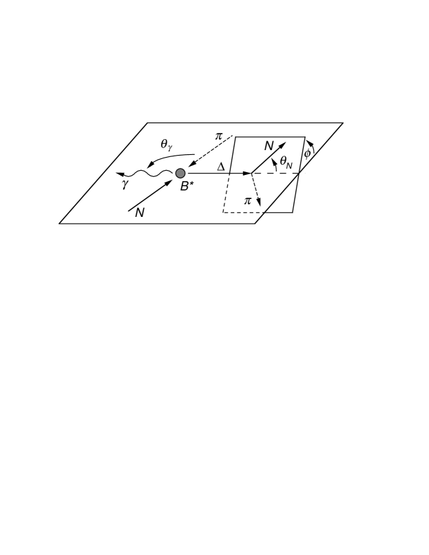
Figure 1: Production and decay of an excited baryon $B^{*}$ in its own rest frame. The angles $\theta_{\gamma}$, $\phi$, and $\theta_{N}$ are indicated. The $\theta_{N}$ used in the text is $\theta_{N}$ boosted to the rest frame of the $\Delta$.

Using the above expression, one can separate $|A_{3/2}|$ and $|A_{5/2}|$. However, $|A_{-1/2}|^{2}$ and $|A_{1/2}|^{2}$ are multiplied by the same kinematic factor, as one can see by substituting $\lambda=\pm 1/2$ and using the symmetry of the $d$-functions in the lower two indices. Hence, some further measurement is needed to separate them.

Recall that the $\Delta$ decays dominantly into $N\pi$, so the full reaction is

$$(\pi{\rm\ or\ }\gamma)+N\rightarrow B^{*}\rightarrow\gamma+\Delta\rightarrow\gamma+N+\pi.$$ (3.14)

The angular distribution of the Delta decay involves two more angles. The decays of the $B^{*}$ and of the $\Delta$ each define a plane, and the angle between them is the azimuthal angle $\phi$. There is also a polar angle $\theta_{N}$, defined in the $\Delta$ rest frame as the angle between the emerging $N$ and the $\Delta$ helicity axis inherited from the $B^{*}$ rest frame. The angular distribution of the $\Delta$ decay depends on its helicity. For example, if the Delta has a definite helicity $\lambda_{\Delta}$, the decay distribution is proportional to

$${1\over 2}\left(1+s_{\lambda}P_{2}(\cos\theta_{N})\right)$$ (3.15)

where $P_{\ell}$ is a Legendre polynomial, and

$$s_{\lambda}=(-1)^{|\lambda_{\Delta}|-1/2}=\left\{\begin{array}[]{ll}+1,&\lambda=1/2,3/2\\ -1,&\lambda=-1/2,5/2\end{array}\right..$$ (3.18)

The last part follows using $\lambda=1-\lambda_{\Delta}$. All four helicity amplitudes can be separated if one measures the angular distributions of the outgoing $N$ (or outgoing $\pi$) in addition to that of the outgoing $\gamma$.

We will give the formulas for the double differential cross sections, including an explicit evaluation of the $d$-functions, separately for $J=1/2$, $3/2$, and $5/2$:

$${d\Gamma_{\gamma}\left(B^{*}_{1/2}\right)\over d\cos\theta_{\gamma}\,d\cos\theta_{N}}={k^{2}\over 4\pi}{m_{\Delta}\over m_{B^{*}}}\left\{\left|A_{-1/2}\right|^{2}\left(1-P_{2}(\cos\theta_{N})\right)+\left|A_{1/2}\right|^{2}\left(1+P_{2}(\cos\theta_{N})\right)\right\},$$

$${d\Gamma_{\gamma}\left(B^{*}_{3/2}\right)\over d\cos\theta_{\gamma}\,d\cos\theta_{N}}={k^{2}\over 4\pi}{m_{\Delta}\over 2m_{B^{*}}} \Bigg{\{} \left|A_{-1/2}\right|^{2}\left(1+[1-2p_{3/2}]P_{2}(\cos\theta_{\gamma})\right)\left(1-P_{2}(\cos\theta_{N})\right)$$

$$+ \left|A_{1/2}\right|^{2}\left(1+[1-2p_{3/2}]P_{2}(\cos\theta_{\gamma})\right)\left(1+P_{2}(\cos\theta_{N})\right)$$

$$+ \left|A_{3/2}\right|^{2}\left(1-[1-2p_{3/2}]P_{2}(\cos\theta_{\gamma})\right)\left(1+P_{2}(\cos\theta_{N})\right)\Bigg{\}},$$

and

$${d\Gamma_{\gamma}\left(B^{*}_{5/2}\right)\over d\cos\theta_{\gamma}\,d\cos\theta_{N}}={k^{2}\over 4\pi}{m_{\Delta}\over 3m_{B^{*}}}\times$$

$$\quad\Bigg{\{}\left|A_{-1/2}\right|^{2}\left(1+{8\over 7}[1-{3\over 4}p_{3/2}]P_{2}(\cos\theta_{\gamma})+{6\over 7}[1-{5\over 2}p_{3/2}]P_{4}(\cos\theta_{\gamma})\right)\left(1-P_{2}(\cos\theta_{N})\right)$$

$$\quad+\left|A_{1/2}\right|^{2}\left(1+{8\over 7}[1-{3\over 4}p_{3/2}]P_{2}(\cos\theta_{\gamma})+{6\over 7}[1-{5\over 2}p_{3/2}]P_{4}(\cos\theta_{\gamma})\right)\left(1+P_{2}(\cos\theta_{N})\right)$$

$$\quad+\left|A_{3/2}\right|^{2}\left(1+{2\over 7}[1-{3\over 4}p_{3/2}]P_{2}(\cos\theta_{\gamma})-{9\over 7}[1-{5\over 2}p_{3/2}]P_{4}(\cos\theta_{\gamma})\right)\left(1+P_{2}(\cos\theta_{N})\right)$$

$$\quad+\left|A_{5/2}\right|^{2}\left(1-{10\over 7}[1-{3\over 4}p_{3/2}]P_{2}(\cos\theta_{\gamma})+{3\over 7}[1-{5\over 2}p_{3/2}]P_{4}(\cos\theta_{\gamma})\right)\left(1-P_{2}(\cos\theta_{N})\right)\Bigg{\}}.$$

Note that we have integrated over the azimuthal angle $\phi$ in deriving these decay widths. We see that we can now extract the magnitude of each of the helicity amplitudes separately, the goal stated at the beginning of this section. It is worth pointing out that we gain some, but not complete, information on the relative signs of the amplitudes by including the azimuthal angle dependence. To determine the remaining signs requires a more detailed analysis, including for example polarizations and/or interference with the nonresonant background; we will consider these issues elsewhere. Again, to use these formulas for the pion induced reaction, set $p_{3/2}=0$.

4 Discussion

The advent of new experimental facilities makes the measurement of excited baryon decay into $\Delta(1232)+\gamma$ a real possibility. In this paper, we have considered decays of the 70-plet. There are 24 new measurable amplitudes for 70 $\rightarrow\Delta\gamma$, not counting amplitudes that are related using isospin invariance.

Until now, the corresponding data on decays into $N\gamma$ has been obtained using time reversal invariance and photoproduction. This possibility doesn’t exist for $\Delta\gamma$ decays, and the lack of data appears to have engendered a paucity of theoretical study. However, measurements of the 70 $\rightarrow\Delta\gamma$ are interesting for several specific reasons.

First, they are a test of the SU(6) symmetry that arises in the large-$N_{c}$ limit for baryons of low spin within any given multiplet. The $\Delta$ and the nucleon are both members of the 56-plet, and thus the 70 $\rightarrow\Delta\gamma$ amplitudes are predictable in terms of the same SU(6)-breaking parameters that determine the 70 $\rightarrow N\gamma$ decays. Considering the one body operators, there are three such parameters, and the fit to the 19 $N\gamma$ decays is decently good. If one assumes, as in the quark model, that only one-body decay operators are relevant, then the predictions for the $\Delta\gamma$ decays given in this paper provide 24 new opportunities to verify or vilify SU(6). Our predictions also provide a means of discerning effects of the most important two-body decay operators, those involving coherent sums over the large-$N_{c}$ baryon states.

Secondly, the 70 $\rightarrow\Delta\gamma$ decays allow us to test the assumption that two-body operators proportional to quark spin sums have matrix elements that are incoherent. Since the $\Delta$ spin is larger than that of the nucleon, it is possible that these subleading effects are not sufficiently suppressed for $N_{c}=3$ to justify the large-$N_{c}$ operator analysis. Then we might encounter large corrections not present in the $N\gamma$ decays. Such large multibody operator effects would lead to significant deviations from the predictions presented here, as well as a noticeable breakdown of the naive quark model.

Acknowledgments

We thank David Armstrong, Nathan Isgur, and Ron Workman for useful comments. CDC thanks the National Science Foundation for support under grant PHY-9800741. CEC thanks the NSF for support under grant PHY-9600415.

References

- [1] G. ’t Hooft, Nucl. Phys. B72, 461 (1974).
- [2] R. Dashen and A. V. Manohar, Phys. Lett. B315, 425 (1993); ibid., 438 (1993).
- [3] E. Jenkins, Phys. Lett. B315, 431 (1993).
- [4] R. Dashen, E. Jenkins, and A. V. Manohar, Phys. Rev. D 49, 4713 (1994).
- [5] C. D. Carone, H. Georgi, and S. Osofsky, Phys. Lett. B322, 227 (1994).
- [6] M. A. Luty and J. March-Russell, Nucl. Phys. B426, 71 (1994).
- [7] E. Jenkins, Phys. Lett. B315, 441 (1993).
- [8] R. F. Dashen, E. Jenkins, and A. V. Manohar, Phys. Rev. D 51, 3697 (1995).
- [9] E. Jenkins and R. F. Lebed, Phys. Rev. D 52, 282 (1995).
- [10] E. Jenkins and A. V. Manohar, Phys. Lett. B335, 452 (1994);
- [11] M. A. Luty, J. March-Russell, M. White, Phys. Rev. D 51, 2332 (1995).
- [12] J. Dai, R. Dashen, E. Jenkins, and A. V. Manohar, Phys. Rev. D 53, 273 (1996).
- [13] J. L. Goity, Phys. Lett. B414, 140 (1997).
- [14] C. E. Carlson, C. D. Carone, J. L. Goity, and R. F. Lebed, hep-ph/9807334, submitted to Phys. Lett. B.
- [15] C. D. Carone, H. Georgi, L. Kaplan, and D. Morin, Phys. Rev. D 50, 5793 (1994).
- [16] D. Pirjol and T.-M. Yan, Phys. Rev. D 57, 5434 (1998).
- [17] D. Pirjol and T.-M. Yan, Phys. Rev. D 57, 1449 (1998).
- [18] C. E. Carlson and C. D. Carone, Phys. Rev. D 58 053005 (1998).
- [19] See, for example, L. A. Copley, G. Karl and E. Obryk, Phys. Lett. B29, 117 (1969); Nucl. Phys. B13, 303 (1969).
- [20] For an exception, see F. J. Gilman and I. Karliner, Phys. Rev. D 10, 2194 (1974).
- [21] Particle Data Group, C. Caso, et al., Eur. Phys. J. C3 1, (1998).
- [22] F.E. Close, Quarks and Partons, Academic Press, London, 1979.
- [23] A. R. Edmonds, Angular Momentum in Quantum Mechanics, Princeton University Press, Princeton, 1960.