Neutrino conversions in random magnetic fields and $\tilde{\nu}_{e}$ from the Sun

Abstract

The magnetic field in the convective zone of the Sun has a random small-scale component with the r.m.s. value substantially exceeding the strength of a regular large-scale field. For two Majorana neutrino flavors $\times$ two helicities in the presence of a neutrino transition magnetic moment and nonzero neutrino mixing we analyze the displacement of the allowed ($\Delta m^{2}$-$\sin^{2}\theta$)- parameter region reconciled for the SuperKamiokande(SK) and radiochemical (GALLEX, SAGE, Homestake) experiments in dependence on the r.m.s. magnetic field value $b$, or more precisely, on a value $\mu b$ assuming the transition magnetic moment $\mu=10^{-11}\mu_{B}$. In contrast to RSFP in regular magnetic fields we find an effective production of electron antineutrinos in the Sun even for small neutrino mixing through the cascade conversions $\nu_{eL}\to\nu_{\mu L}\to\tilde{\nu}_{eR}$, $\nu_{eL}\to\bar{\nu}_{\mu R}\to\bar{\nu}_{eR}$ in a random magnetic field that would be a signature of the Majorana nature of neutrino if $\tilde{\nu}_{eR}$ will be registered. Basing on the present SK bound on electron antineutrinos we have also found an excluded area in the same $\Delta m^{2}$, $\sin^{2}2\theta$ -plane and revealed a strong sensitivity to the random magnetic field correlation length $L_{0}$.

I Introduction

Recent results of the SuperKamiokande (SK) experiment[1] have already confirmed the solar neutrino deficit at the level less $R_{SK}/R_{SSM}\;\raise 1.29167pt\hbox{$<$\kern-7.5pt\raise-4.73611pt\hbox{$\sim$}}\;0.4$.

Moreover, day/night (D/N) and season neutrino flux variations were analized in this experiment and in $\approx$ 4 years one expects to reach enough statistics in order to confirm or to refuse these periods predicted in some theoretical models. D/N variations would be a signature of the MSW solution to the Solar Neutrino Problem (SNP). The signature of the vacuum oscillations is a seasonal variation of neutrino flux, in addition to geometrical seasonal variation $1/r^{2}(t)$. And signature of the resonant spin-flavor precession (RSFP)-solution is the 11 year periodicity of neutrino flux.

All three elementary particle physics solutions (vacuum, MSW and RSFP) successfully describe the results of all four solar-neutrino experiments, because the suppression factors of neutrino fluxes are energy dependent and helioseismic data confirm the Standard Solar Model (SSM) with high precision at all radial distances of interest (see recent review by Berezinsky [2]).

There exists, however, a problem with large regular solar magnetic fields, essential for the RSFP scenario. It is commonly accepted that magnetic fields measured at the surface of the Sun are weaker than within interior of the convective zone where this field is supposed to be generated. The mean field value over the solar disc is about of order $1~{}G$ and in the solar spots magnetic field strength reaches $1~{}kG$.

Because sunspots are considered to be produced from magnetic tubes transported to the solar surface due to the boyancy, this figure can be considered as a reasonable order-of magnitude observational estimate for the mean magnetic field strength in the region of magnetic field generation. In the solar magnetohydrodynamics (see e.g. [3])) one can explain such fields in a self-consistent way if these fields are generated by dynamo mechanism at the bottom of the convective zone (or, more specific, in the overshoot layer). But its value seems to be too low for effective neutrino conversions.

The mean magnetic field is however followed by a small scale, random magnetic field. This random magnetic field is not directly traced by sunspots or other tracers of solar activity. This field propagates through convective zone and photosphere drastically decreasing in the strength value with an increase of the scale. According to the available understanding of solar dynamo, the strength of the random magnetic field inside the convective zone is larger than the mean field strength. A direct observational estimation of the ratio between this strengthes is not available, however the ratio of order 50 – 100 does not seem impossible. At least, the ratio between the mean magnetic field strength and the fluctuation at the solar surface is estimated as 50 (see e.g. [4]).

This is the main reason why we consider here an analogous to the RSFP scenario, an aperiodic spin-flavour conversion (ASFC), based on the presence of random magnetic fields in the solar convective zone. It turns out that the ASFC is an additional probable way to describe the solar neutrino deficit in different energy regions, especially if current and future experiments will detect electron antineutrinos from the Sun. The termin “aperiodic” simply reflects the exponential behaviour of conversion probabilities in noisy media (cf. [5] , [6]).

As well as for the RSFP mechanism[7] all arguments for and against the ASFC mechanism with random magnetic fields remain the same ones that have been recently summarized and commented by Akhmedov (see [8] and references therein).

But contrary to the case of regular magnetic fields we find out that one of the signatures of random magnetic field in the Sun is the prediction of a wider allowed region for neutrino mixing angle in the presence of $\bar{\nu}_{e}$ from the Sun including the case of small mixing angles (see below section IV).

Notice that if electron antineutrinos from the Sun were detected at the Earth this would lead to conclusion that neutrinos are Majorana particles and this is a very attractive point for applying RSFP in regular magnetic field or ASFC in random fields in the Sun.

The SK experiment provides a stringent bound on the presence of solar electron antineutrinos at least for high energy region [9]. A phenomenological and numerical analysis of $\nu_{eL}\to\tilde{\nu}_{eR}$-conversion in the solar twisting magnetic fields [10] - [12] shows that it is possible to obtain a noticeable yield of $\tilde{\nu}_{eR}~{}$ [11] consistent with the limit [9]. Twisting magnetic fields themselves are, however, very specific and it is hard to explain their existence and origin. Therefore, more realistic models of magnetic field in the Sun are necessary and for a start we treat here both SNP solution and $\tilde{\nu}_{e}$-production applying, as we hope, a bit more realistic model of random magnetic fields in the convective zone of the Sun.

The random magnetic field is considered to be maximal somewhere at the bottom of convective zone and decaying to the solar surface. To take into account a possibility, that the solar dynamo action is possible also just below the bottom of the convective zone (see [3]), we accept, rather arbitrary, that it is distributed at the radial range $0.7R_{\odot}\mbox{---}1.0R_{\odot}$, i.e. it has the same thickness as the convective zone. Of course, our model of the random magnetic field (see in details below) is a crude simplification of the real situation, however, the results are presumably more or less robust.

For each realization of random magnetic fields we find a solution of the Cauchi problem in the form of a set of wave functions $\nu_{a}(t)=\mid\nu_{a}(t)\mid\exp(i\alpha_{a}(t))$ obeying the unitarity condition for the probabilities $P_{aa}(t)=\nu_{a}^{*}(t)\nu_{a}(t)$,

$$P_{ee}(t)+P_{\bar{e}\bar{e}}(t)+P_{\mu\mu}(t)+P_{\bar{\mu}\bar{\mu}}(t)=1~{},$$ (1)

where the subscript $a$ equals to $a=e$ for $\nu_{eL}$, $a=\bar{e}$ for $\bar{\nu}_{eR}$, $a=\mu$ for $\nu_{\mu L}$ and $a=\bar{\mu}$ for $\bar{\nu}_{\mu R}$ correspondingly.

In section II the experimental observables are defined through the neutrino conversion probabilities $P_{aa}(E)$ at the detectors ($r=R_{Earth}$) accounting for neutrino propagation both in the Sun and on the way from the Sun to the Earth.

In subsection II.A we give general formulas for the neutrino event spectrum in real time experiments with measurement of recoil electron energy in the $\nu e$-scattering. In contrast to the well-known case of regular fields, we need to find the probabilities $P_{aa}(r=t)$ as the functions of a local position in the transversal plane too, $P_{aa}(r)\equiv P_{aa}(r,\xi,\eta)$, because longitudinal profiles of the random fields (along $r$) are generally different in different points in the transversal plane even for an instant when parallel neutrino fluxes directed to the Earth (called here ”rays”) cross the convective zone (see Fig. 1).

As a result of different realizations of random fields along different rays the probabilities $P_{aa}(r,\xi,\eta)$ are random functions built on randomness of magnetic fields in all three directions.

The same probabilities for left-handed electron neutrinos, $P_{ee}(r,\xi,\eta)$, are used in subsection II.B to define neutrino flux measured in radiochemical experiments (Homestake and GALLEX + SAGE, in SNU units).

In main section III we give some physical arguments supporting the random magnetic field model implemented into the master equation Eq. (16) (subsection III.B.1). After that we describe the mathematical model of random magnetic fields (subsection III.B.2).

Then in subsection III.C we analyze asymptotic solution of the master equation in the case of small neutrino mixing. We briefly discuss there many possible analytic issues: in particular, magnetic field correlations of finite radius (subsection III.C.2), linked cluster expansion and higher moments of survival probability (subsection III.C.3). We give also an interpretation of the random magnetic field influence as a random walk over a circle (subsection III.C.4).

In subsection III.D we describe the algorithm of our numerical approach. The main goal is to calculate the mean arithmetic probabilities as functions of mixing parameters $\sin^{2}2\theta$ , $\delta=\Delta m^{2}/4E$,

$$\langle P_{aa}(\delta,\sin^{2}2\theta)\rangle=\int\int d\xi d\eta P_{aa}(\delta,\sin^{2}2\theta,\xi,\eta)/\int\int d\xi d\eta\ ,$$ (2)

under the assumption $\Phi^{(0)}_{i}(\xi,\eta,E)=\Phi^{(0)}_{i}(\xi,\eta)\lambda_{i}(E)$, where $\lambda_{i}(E)$ is the corresponding normalized differential flux, $\int_{0}^{E_{max}(i)}\lambda_{i}(E)dE=1$ and $\Phi^{(0)}_{i}(\xi,\eta)$ is the integral flux of neutrinos of kind ”i” ($i=pp~{},Be~{},pep~{},B$) assumed to be constant and uniform, $\Phi^{(0)}_{i}(\xi,\eta)=\Phi^{(0)}_{i}=const$, at a given distance $r=t$ from the center of the Sun [13]. This simplifies the averaging in the transversal plane since

$$\int_{\xi^{2}+\eta^{2}<R_{core}^{2}}d\xi d\eta\Phi_{i}^{(0)}(\xi,\eta)P_{aa}(\xi,\eta)\times[\int_{\xi^{2}+\eta^{2}<R_{core}^{2}}d\xi d\eta]^{-1}=\Phi^{(0)}_{i}\times\langle P_{aa}\rangle\ .$$ (3)

It is worth to note that the above averaging procedure merely reflects the physical properties of neutrino detectors which response to the incoherent sum of partial neutrino fluxes incoming from all visible parts of the Sun. At the same time it is well known that the most studied statistical characteristics in statistical physics and especially in the theory of disordered media are those that are additive functions of dimensions (cf. [14]). Their main distinctive feature is that, being devided by corresponding volume, they become certain in macroscopic limit, i.e. self-averaged. From definition Eq. (2) it follows that the integral in the numerator in the r.h.s. is indeed an additive function of the area of the convective zone layer (see also Fig. 1) and therefore for increasing area one can expect that $\langle P_{aa}\rangle$ should be self-averaged. Our results below confirm this property ( subsection III.C.3 and section IV).

In section IV we analyze how these probabilities depend on the r.m.s. field value $\sqrt{\langle b^{2}\rangle}$ and argue why electron antineutrinos are not seen in the SK experiment reconciling available experimental data for four solar neutrino experiments.

In final section V we discuss our results comparing two mechanisms, RSFP and ASFC, for the same strength of regular and r.m.s. fields and $\mu=10^{-11}\mu_{B}$.

II Experimental observable values

If neutrinos have the transition magnetic moment, then in real time experiments like $\nu$e-scattering in the SK case[1] the recoil electron spectrum depends on all four neutrino conversion probabilities, $P_{aa}$ (see subsection II.A), while in the case of radiochemical experiments (Homestake, Gallex, SAGE[16]) the number of events measured in SNU units depends on charge current contribution with left-handed electron neutrinos only, i.e. on the survival probability $P_{ee}$ that itself is a function of the magnetic field parameter $\mu B_{\perp}$, as well as of the fundamental mixing parameters $\Delta m^{2}$, $\sin^{2}2\theta$ (subsection II.B).

A Spectrum and number of neutrino events in $\nu e$-scattering experiments

In a real time experiment one measures the integral spectrum (the number of neutrino events per day)

$$N_{\nu}=\sum_{k_{min}}^{k_{max}}\int_{T_{k}}^{T_{k+1}}dT\frac{dN_{\nu}(T)}{dT}~{},$$ (4)

where experimentalists devide the whole allowed recoil electron energy interval $T\geq T_{th}$ into bins $\Delta W=T_{k+1}-T_{k}$ with $T_{k_{min}}=T_{th}$. The energy spectrum of events, $dN_{\nu}/dT$, has the form

$$\frac{dN_{\nu}}{dT} = N_{e}[\int\int_{\xi^{2}+\eta^{2}<R_{core}^{2}}d\xi d\eta]^{-1}\times\int_{\xi^{2}+\eta^{2}<R_{core}^{2}}d\xi d\eta\sum_{i}\Phi^{(0)}_{i}(\xi,\eta)\times$$ (6)

$$\int_{E_{min}(T)}^{E_{max}(i)}dE\varepsilon(E)\lambda_{i}(E)\langle\frac{d\sigma^{(M)}_{weak}}{dT}(E,T||\xi,\eta)\rangle~{},$$

where $N_{e}$ is the total number of electrons in the fiducial volume of the detector; $E_{min}(T)=(T/2)(1+\sqrt{1+2m_{e}/T})$ is the minimal neutrino energy obtained from the kinematical inequality $T\leq T_{max}=2E^{2}/(2m_{e}+2E)$ and $E_{max}(i)$ is given in [13]. For simplicity the efficiency $\varepsilon(E)$ above the detector threshold $T_{th}$ is substituted by $\varepsilon(E)=1$.

Notice that we have assumed the same core radii for all neutrino sources (kinds ”i”), $R_{core}=R_{core}^{(i)}$.

The averaged differential cross-section $\langle d\sigma^{(M)}_{weak}(E,T||\xi,\eta)/dT\rangle$ in Eq. (6),

$$\langle\frac{d\sigma^{(M)}_{weak}}{dT}(E,T||\xi,\eta)\rangle=\Bigl{[}\int_{0}^{T_{max}}\exp(-(T-T^{{}^{\prime}})^{2}/2\Delta(T^{{}^{\prime}})^{2})dT^{{}^{\prime}}\Bigr{]}^{-1}\times$$ (7)

$$\times\Bigl{[}\int_{0}^{T_{max}}\exp(-(T-T^{{}^{\prime}})^{2}/2\Delta(T^{{}^{\prime}})^{2})dT^{{}^{\prime}}\frac{d\sigma^{(M)}_{weak}(T^{{}^{\prime}},E||\xi,\eta)}{dT^{{}^{\prime}}}\Bigr{]}$$ (8)

is given by the energy resolution $\Delta T\equiv\Delta(T)$ in the Gaussian distribution where $T^{{}^{\prime}}$ is the true recoil electron energy, $T$ is the measured energy, and by the $\nu e$ scattering cross-section for four active Majorana neutrino components[15]

$$\frac{d\sigma^{(M)}_{weak}(E,T^{{}^{\prime}}||\xi,\eta)}{dT}=\frac{2G_{F}^{2}m_{e}}{\pi}\{P_{ee}(E,\xi,\eta) \Bigl{[}g_{eL}^{2}+g_{R}^{2}\Bigl{(}1-\frac{T^{{}^{\prime}}}{E}\Bigr{)}^{2}-\frac{m_{e}T^{{}^{\prime}}}{E^{2}}g_{eL}g_{R}\Bigr{]}+$$ (9)

$$+P_{\bar{e}\bar{e}}(E,\xi,\eta) \Bigl{[}g_{R}^{2}+g_{eL}^{2}\Bigl{(}1-\frac{T^{{}^{\prime}}}{E}\Bigr{)}^{2}-\frac{m_{e}T^{{}^{\prime}}}{E^{2}}g_{eL}g_{R}\Bigr{]}+$$ (10)

$$+P_{\mu\mu}(E,\xi,\eta) \Bigl{[}g_{\mu L}^{2}+g_{R}^{2}\Bigl{(}1-\frac{T^{{}^{\prime}}}{E}\Bigr{)}^{2}-\frac{m_{e}T^{{}^{\prime}}}{E^{2}}g_{\mu L}g_{R}\Bigr{]}+$$ (11)

$$+P_{\bar{\mu}\bar{\mu}}(E,\xi,\eta) \Bigl{[}g_{R}^{2}+g_{\mu L}^{2}\Bigl{(}1-\frac{T^{{}^{\prime}}}{E}\Bigr{)}^{2}-\frac{m_{e}T^{{}^{\prime}}}{E^{2}}g_{\mu L}g_{R}\Bigr{]}\}~{}.$$ (12)

Here $g_{eL}=\xi+0.5$, $g_{\mu L}=\xi-0.5$, $g_{R}=\xi=\sin^{2}2\theta_{W}\simeq 0.23$ are the coupling constants in the Standard Model(SM).

Let us stress that a specific dependence of probabilities on the transversal coordinates $\xi~{},\eta$ vanishes for a homogeneous regular magnetic field which is a function of the longitudinal coordinate $r=t$ only. Therefore for scenarios with regular fields (for instance, in [7]) the spectrum Eq. (6) takes the usual form without dependence on transversal coordinates.

If we assume uniform partial neutrino fluxes, the integration over the transversal coordinates $\xi,~{}\eta$ in the integrand of the event number Eq. (6) leads to the averaging of probabilities, see Eq. (3) and subsection III.D.

The energy resolution in the SK experiment is given by $\Delta(T)=\Delta_{10}\sqrt{T/10~{}MeV}$ and for the Kamiokande experiment is estimated as $\Delta T/T\sim 0.2$ at the energy $T=10~{}MeV$, or $\Delta_{10}=2~{}MeV$. This irreducible systematical error becomes even worse near the threshold ($T_{th}=6.5~{}MeV$ at the present time and one plans to reach $T_{th}=5~{}MeV$ in 1998).

In BOREXINO (starts in 1999), where one has a liquid scintillator, it is expected to observe approximately 300 photoelectrons (phe) per $MeV$ of deposited recoil electron energy. This gives an estimate of the energy resolution of the order[17]

$$\frac{\Delta T}{T}(BOREXINO)\simeq\frac{1}{\sqrt{N_{phe}}}\simeq\frac{0.058}{\sqrt{T/MeV}}~{},$$ (13)

corresponding to 12 % for the threshold ($T_{th}\simeq 0.25~{}MeV$) and 7 % for the maximum recoil energy for Be neutrinos, $T_{max}\simeq 0.663~{}MeV$.

In HELLAZ the Multi-Wire-Chamber (MWC) counts the secondary electrons produced by the initial one in helium. It is expected to count 2500 electrons at the threshold energy $T_{th}\simeq 0.1~{}MeV$, so in that case[18]

$$\frac{\Delta T}{T}(HELLAZ)\simeq\frac{1}{\sqrt{N_{e}}}\simeq\frac{0.02}{\sqrt{T/T_{th}}}~{},$$ (14)

or the energy resolution of the order 1.5 % for the maximum for $pp$ neutrinos $T_{max}\simeq 0.26~{}MeV$.

Other experimental uncertainties must be incorporated into the differential spectra Eq. (6). We have neglected an unknown statistical error, which we expect to be less than the systematical one after enough exposition time, as it will decrease as $\mid\pm\Delta N_{\nu}/N_{\nu}\mid\sim t^{-1/2}$. We have also neglected inner and external background contributions to the systematical error considering them as the specifical ones for each experiment.

B Radiochemical experiments

The number of neutrino events in GALLEX (SAGE) and Homestake experiments measured in SNU (1 SNU = $10^{-36}$ captures per atom/per sec) has the form

$$10^{-36}N^{\nu}_{Ga,~{}Cl}=\sum_{i}\Phi^{(0)}_{i}\int_{E_{th}(Ga,Cl)}^{E_{max}(i)}\lambda_{i}(E)\sigma_{Ga,~{}Cl}(E)<P_{ee}(E)>\,dE~{},$$ (15)

where the thresholds $E_{th}(Ga,Cl)$ for GALLEX (SAGE) and Homestake are $0.233~{}MeV$ and $0.8~{}MeV$ correspondingly and the capture cross sections $\sigma_{Ga,~{}Cl}(E)$ for gallium and clorine detectors are tabulated in [13], see Table 8.4.

For $P_{ee}=1$ the SSM predictions for radiochemical experiments are listed in the Table 8.2. [13]. For updated theoretical fluxes in BP95 model[19] we find the mean SSM predictions 137 SNU for GALLEX (SAGE) and 9,3 SNU for the Homestake experiment. The experimental data[16] pronounce the electron neutrino deficit, $69.7\pm 6.7^{+3.9}_{-4.5~{}}$SNU for the GALLEX, $69\pm 10^{+5}_{-7~{}}$SNU for the SAGE and $2.55\pm 0.17\pm 0.18~{}$SNU for the Homestake experiments.

Notice that the ratio of the experimental data to SSM predictions above does not depend on theoretical uncertainties of the integral neutrino fluxes, $\Phi^{(0)}_{i}$, in Eq. (15). Neutrino deficit expressed through these ratios[2] is $0.509\pm 0.059$, $0.504\pm 0.085$ and $0.274\pm 0.027$ for GALLEX, SAGE and Homestake correspondingly where the experimental 1$\sigma$-errors come from $\sqrt{\sigma^{2}_{stat}+\sigma^{2}_{sys}}$.

III Master equation and its solution

A Master equation

We consider conversions $\nu_{eL,R}\to\nu_{aL,R}$, $a=\mu$ or $\tau$, for two neutrino flavors obeying the master evolution equation

$$i\left(\begin{array}[]{l}\dot{\nu}_{eL}\\ \dot{\tilde{\nu}}_{eR}\\ \dot{\nu}_{\mu L}\\ \dot{\tilde{\nu}}_{\mu R}\end{array}\right)=\left(\begin{array}[]{cccc}V_{e}-c_{2}\delta&0&s_{2}\delta&\mu H_{+}(t)\\ 0&-V_{e}-c_{2}\delta&-\mu H_{-}(t)&s_{2}\delta\\ s_{2}\delta&-\mu H_{+}(t)&V_{\mu}+c_{2}\delta&0\\ \mu H_{-}(t)&s_{2}\delta&0&-V_{\mu}+c_{2}\delta\end{array}\right)\left(\begin{array}[]{c}\nu_{eL}\\ \tilde{\nu}_{eR}\\ \nu_{\mu L}\\ \tilde{\nu}_{\mu R}\end{array}\right)~{},$$ (16)

where $c_{2}=\cos 2\theta$, $s_{2}=\sin 2\theta$, $\delta=\Delta m^{2}/4E$ are the neutrino mixing parameters; $\mu=\mu_{12}$ is the neutrino active-active transition magnetic moment; $H_{\pm}(t)=B_{0\pm}(t)+b_{\pm}(t)$, $H_{\pm}=H_{x}\pm iH_{y}$, are the magnetic field components consisting of regular ($B_{0\pm}$) and random ($b_{\pm}$) parts which are perpendicular to the neutrino trajectory in the Sun; $V_{e}(t)=G_{F}\sqrt{2}(\rho(t)/m_{p})(Y_{e}-Y_{n}/2)$ and $V_{\mu}(t)=G_{F}\sqrt{2}(\rho(t)/m_{p})(-Y_{n}/2)$ are the neutrino vector potentials for $\nu_{eL}$ and $\nu_{\mu L}$ in the Sun given by the abundances of the electron ($Y_{e}=m_{p}N_{e}(t)/\rho(t)$) and neutron ($Y_{n}=m_{p}N_{n}(t)/\rho(t)$) components and by the SSM density profile $\rho(t)=250~{}g/cm^{3~{}}\exp(-10.54t)$ [13].

Notice that we did not assume here a twist field model with analogous constructions $B_{\pm}=B_{x}\pm iB_{y}$ in off-diagonal entries of the Hamiltonian in Eq. (16) These expressions are derived from the initial Majorana equations in the mass-eigenstate representation where transversal part of the spin-flip term $\mu\vec{\sigma}\cdot\vec{B}$ leads automatically to the ”twist-form” in the Schrödinger equation above written in flavor representation (see [20]). We have not performed the phase transform of the Hamiltonian in Eq. (16) since, in contrast to [10], the phase $\Phi(t)$ in $H_{\pm}=H_{\perp}(t)e^{\pm i\Phi(t)}$ is the random one that gives uncertainty in the additional term $\dot{\Phi}$ for the resonance condition [10]. Instead of that we have solved Eq. (16) directly using computer simulation (see below).

B Solar magnetic fields

1 Random magnetic fields

The r.m.s. random component b is assumed to be stronger then the regular one, B, and maybe even much stronger than $B_{0}$, $\langle b^{2}\rangle\gg B_{0}^{2}$, provided the large magnetic Reynolds number $R_{m}$ leads to the effective dynamo enhancement of small-scale (random) magnetic fields.

Let us give simple estimates of the magnetic Reynolds number $R_{m}=lv/\nu_{m}$ in the convective zone for fully ionized hydrogen plasma ($T\gg I_{H}\sim 13.6~{}eV\sim 10^{5}~{}K$). Here $l\sim 10^{8}~{}cm$ is the size of eddy (of the order of magnitude of a granule size) with the turbulent velocity inside of it $v\sim 10^{5}~{}cm/s$. Provided an equipartition between the turbulent kinetic energy and the mean magnetic field is suggested, we obtain $v\approx v_{A}=B/\sqrt{4\pi\rho}$, where $v_{A}$ is the Alfven velocity for MHD plasma, $B$ is the mean (large-scale) magnetic field in convective zone and $\rho$ is the matter density The magnetic diffusion coefficient, or magnetic viscosity, $\nu_{m}=c^{2}/4\pi\sigma_{cond}$ entering the diffusion term of the Faradey induction equation,

$$\frac{\partial{\bf\vec{H}}}{\partial t}=rot[{\bf\vec{v}}\times{\bf\vec{H}}]+\nu_{m}\Delta{\bf\vec{H}}~{},$$ (17)

where ${\bf\vec{H}}={\bf\vec{B}}+{\bf\vec{b}}$ is the total magnetic field (mean field plus fluctuations), is given by the conductivity of the hydrogen plasma $\sigma_{cond}=\omega_{pl}^{2}/4\pi\nu_{ep}$. Here $c$ is the light velocity; $\omega_{pl}=\sqrt{4\pi e^{2}n_{e}/m_{e}}=5.65\times 10^{4}\sqrt{n_{e}}~{}s^{-1}$ is the plasma, or Lengmuir frequency; $\nu_{ep}=50n_{e}/T^{3/2}~{}s^{-1}$ is the electron-proton collision frequency; and the electron density $n_{e}=n_{p}$ and the temperature $T$ are measured in $cm^{-3}$ and Kelvin degrees respectively.

It follows that the magnetic diffusion coefficient $\nu_{m}\simeq 10^{13}(T/1~{}K)^{-3/2}~{}cm^{2}s^{-1}$ does not depend on the charge density $n_{e}$ and it is very small for hot plasma $T\geq 10^{5}~{}K$. From comparison of the first and second terms in the r.h.s. of the Faradey equation Eq. (17) we find that $v/l\gg\nu_{m}/l^{2}$, or $\nu_{m}\ll vl\sim 10^{13}~{}cm^{2}s^{-1}$ since $T/1~{}K\gg 1$. This means that magnetic field in the Sun is frozen-in.

As the result we obtain $R_{m}=lv\omega_{pl}^{2}/(c^{2}\nu_{ep})\simeq(10^{-13}lv/cm^{2}s^{-1})(T/1~{}K)^{3/2}$. A standard estimation for $R_{m}$ in the solar convective zone is $R_{m}=10^{8}$ (see [21]).

The estimation of $b/B$ for the solar convective zone (and other cosmic dynamos) is the matter of current scientific discussions. The most concervative estimate, simply based on equipartition concept, is $b=const\,B$. According to direct observations of galactic magnetic field presumably driven by a dynamo, $b\approx 1.8B$ ([22]). A more developed theory of equipartition gives, say, $b=constB\ln R_{m}$ (see [21]). For our consideration taking this constant as $4\pi$ would be more than sufficient.

Notice that this estimate is considered now as very concervative. Basing on more detailed theories of MHD turbulence estimates like $b\sim\sqrt{R_{m}}B$ are discussed [23], [24]. Such estimates give a free room for a very large values of $b$. Let us stress, however, that the larger estimate of $b$ is accepted, the more difficult is to refer for a dynamo as an origin for $B$, so the estimates of Vainstein and Cataneo, [23] and [24] are hardly comparable with the dynamo nature of large-scale solar magnetic field.

Being interested in neutrino conversions, we need only a partial information concerning the small-scale magnetic fields. In particular, because of the very rapid propagation of neutrino in comparison with MHD timescales, we are interesting only in a $b$ distribution at a given instant in a given direction.

2 The model of the magnetic field

The assumed profile of a random magnetic field is presented in the Fig. 2.

We also show there the profile of the regular magnetic field used in calculations. We find that RSFP results are not sensitive to the profile of a regular field. However, switching on random fields, we find out an essential change of the probabilities $P_{aa}(t)$ for the same mixing parameters $\sin^{2}2\theta$, $\Delta m^{2}/2E$. This difference of the magnetic field model influence on the solution of the master equation Eq. (16) becomes the more significant the larger the r.m.s. value $b$ is assumed.

The numerical implementation for the random magnetic field has been chosen as follows. We choose the correlation length for the random field component as $L_{0}=10^{4}~{}km$ that is close to the mesogranule size.

Then we suppose that all the volume of the convective zone is covered by a net of rectangular domains where the random magnetic field strength vector is constant. The magnetic field strength changes smoothly at the boundaries between the neighbour domains obeying the Maxwell equations. Since one can not expect the strong influence of small details in the random magnetic field within and near thin boundary layers between the domains this oversimplified model looks applicable.

In agreement with the SSM [13] we suppose that the neutrino source inside the Sun is located inside the core with the radius of the order of $R_{\nu}=0.1R_{\odot}=7\times 10^{4}~{}km$ and neglect for the sake of simplicity the spatial distribution of neutrino emissivity from a unit of a solid angle of the core image. However, different parallel trajectories directed to the Earth cross different magnetic domains because the domain size $L_{0}$ (in the plane which is perpendicular to neutrino trajectories) is much less than the transversal size $=R_{\nu}$ of the full set of parallel rays, $L_{0}\ll R_{\nu}$. The whole number of trajectories (rays) with statistically independent magnetic fields is about $R_{\nu}^{2}/L_{0}^{2}\sim 50$.

Thus, the perpendicular components $b_{x,y}(r)$ along one representive ray are the random functions with the correlation length $L_{0}$ (see Fig. 2).

At the stage of the numerical simulation of the random magnetic field we generate the set of the random numbers with the given r.m.s. $\sqrt{\langle b^{2}\rangle}$ and suppose that the strength of the random field is constant inside the rectangular volume with the radial size $L_{0}$ and with the same diameter $L_{0}$ in the $\xi~{},\eta$-plane. We assume that $\sqrt{\langle b_{x}^{2}\rangle}=\sqrt{\langle b_{y}^{2}\rangle}$.

We generate random values of $\bf b$ in different cells both along the neutrino trajectory and in the transversal plane $\xi~{},\eta$, solve the Cauchy problem for 50 rays and calculate the mean probabilities Eq. (2).

Notice that we substitute into the integrand of the neutrino event number $dN_{\nu}/dT$ the probabilities $P_{aa}(r=R_{E\odot},\xi,\eta)$ at the Earth taking into account also vacuum neutrino oscillation probabilities (for zero magnetic fields and zero density in the solar wind) and neglecting the Earth effects for relatively small $\Delta m^{2}\sim 10^{-8}~{}eV^{2}$ ($l_{v}=2.48\times 10^{-3}E(MeV)/\Delta m^{2}(eV^{2})~{}km\gg l_{0}=3.28\times 10^{4}~{}km/\rho(g/cm^{3})$
for $\rho\sim 4.5--11~{}g/cm^{3}$ in the Earth). As for MSW-region $\Delta m^{2}\sim 10^{-5}~{}eV^{2}$ we do not consider here the possible Earth influence which could result in day-night variations.

C Asymptotic solution of the master equation

Let us consider how random magnetic field influences the small-mixing MSW solution to SNP with the help of some simplified analytical solutions of the master equation Eq. (16). Indeed, it turns out that for the SSM exponential density profile, typical borone neutrino energies $E\sim 7\div 14MeV$, and $\triangle m^{2}\sim 10^{-5}~{}eV^{2}$, the MSW resonance (i.e. the point where $V_{e}-V_{\mu}=2c_{2}\delta)$ occurs well below the bottom of the convective zone. Thus we can divide the neutrino propagation problem and consider two successive stages. First, after generation in the middle of the Sun, neutrinos propagate in the absence of any magnetic fields, undergo the non-adiabatic (non-complete) MSW conversion $\nu_{eL}\to\nu_{\mu L}$ and acquire certain nonzero values $P_{ee}$ end $P_{\mu\mu}$, which can be treated as initial conditions at the bottom of the convective zone. For small neutrino mixing $s_{2}\to 0$ the $(4\times 4)$-master equation Eq.(8) then splits into two pairs of independent equations describing correspondingly the spin-flavor dynamics $\nu_{el}\to\tilde{\nu}_{\mu R}$ and $\nu_{\mu L}\to\tilde{\nu}_{eR}$ in noisy magnetic fields. In addition, once the MSW resonance point is far away from the convective zone, one can also omit $V_{e}$ and $V_{\mu}$ in comparison with $c_{2}\delta$. For $\nu_{eL}\to\tilde{\nu}_{\mu R}$ conversion this results into a two-component Schr$\rm\ddot{o}$dinger equation

$$i\left(\begin{array}[]{c}\dot{\nu}_{eL}\\ \dot{\tilde{\nu}}_{\mu R}\end{array}\right)\simeq\left(\begin{array}[]{cc}-\delta&\mu b_{+}(t)\\ \mu b_{-}(t)&\delta\end{array}\right)\left(\begin{array}[]{c}\nu_{eL}\\ \tilde{\nu}_{\mu R}\end{array}\right)$$ (18)

with initial conditions $|\nu_{eL}|^{2}(0)=P_{ee}(0),\quad|\tilde{\nu}_{\mu R}|^{2}=P_{\tilde{\mu}\tilde{\mu}}(0)=0.$ As normalized probabilities $P_{ee}(t)$ and $P_{\tilde{\mu}\tilde{\mu}}(t)$ (satisfying the conservation law $P_{ee}(t)+P_{\tilde{\mu}\tilde{\mu}}(t)=P_{ee}(0)$) are the only observables, it is convenient to recast the Eq.(18) into an equivalent integral form

$$S(t) = S(0)-4\mu^{2}\int\limits_{0}^{t}dt_{1}\int\limits_{0}^{t_{1}}dt_{2}S(t_{2})$$ (21)

$$\{[b_{x}(t_{1})b_{x}(t_{2})+b_{y}(t_{1})b_{y}(t_{2})]\cos 2\delta(t_{1}-t_{2})$$

$$-[b_{x}(t_{1})b_{y}(t_{2})-b_{x}(t_{2})b_{y}(t_{1})]\sin 2\delta(t_{1}-t_{2})\},$$

where $S(t)=2P_{ee}(t)-P_{ee}(0)\equiv P_{ee}(t)-P_{\tilde{\mu}\tilde{\mu}}(t)$ is the third component of the polarization vector $\vec{S}$.

1 $\delta$-correlations

If $L_{0}$ is the minimal physical scale in the problem, we can consider random magnetic fields as $\delta$-correlated:

$$<b_{x}(t_{1})b_{x}(t_{2})+b_{y}(t_{1})b_{y}(t_{2})> = \frac{2}{3}<{\vec{b}}^{2}>\cdot L_{0}\delta(t_{1}-t_{2}),$$ (22)

$$<b_{x}b_{y}> = 0.$$ (23)

In this case it turns out that averaging of the Eq.(21) over random magnetic fields is exactly equivalent to averaging of its solution (cf. [6]). The result reads:

$$<S(t)>=S(0)e^{-\Gamma t},$$ (24)

where $<S(t)>$ is the mean value, and decay factor

$$\Gamma=\frac{4}{3}\mu^{2}<\vec{b}^{2}>L_{0}.$$ (25)

If time is measured in units of $L_{0}$ (recall that $c=1$), supposing that neutrino traversed $N$ correlation cells, i.e. $t=L_{0}\times N$, we have

$$<S(N)>=S(0)\exp\left\{-\frac{4}{3}\mu^{2}<\vec{b}^{2}>L_{0}^{2}\times N\right\},$$ (26)

so that N plays a role of an extensive variable like the volume $V$ in statistical mechanics.

2 Correlations of finite radius

Let us consider Eq.(21) in a spirit of our numerical method. Dividing the interval of integration into a set of equal intervals of correlation length $L_{0},$ for a current cell $n$ we have

$$S_{n}\equiv S(n\cdot L_{0})=$$ (27)

$$=S(0)-4\mu^{2}\sum\limits^{n}_{k=1}\sum\limits^{k}_{l=1}\int\limits^{kL_{0}}_{(k-1)L_{0}}dt_{1}\int\limits^{\min\{t_{1},lL_{0}\}}_{(l-1)L_{0}}dt_{2}\;\{\mbox{the integrand of Eq.(\ref{(03)})}\}.$$ (28)

Assuming now that possible correlations between $S(t_{2})$ and $b_{i},b_{j}$ under the integral are small, $S(t)$ itself varies very slowly within one correlation cell (see, however, below), and making use of statistical properties of random fields, ($i$) different transversal components within one cell are independent random variables, and ($ii$) magnetic fields in different cells do not correlate, we can average Eq.(28) thus obtaining a finite difference analogue:

$$S_{n}=S(0)-4\mu^{2}\sum\limits^{n}_{k=1}<\vec{b}_{\perp k}^{2}>S_{k}\int\limits^{kL_{0}}_{(k-1)L_{0}}dt_{1}\int\limits^{t_{1}}_{(k-1)L_{0}}dt_{2}\cos 2\delta(t_{1}-t_{2})=$$ (29)

$$=S(0)-2\mu^{2}\frac{\sin^{2}\delta L_{0}}{\delta^{2}}\sum\limits^{n}_{k=1}<\vec{b}^{2}_{\perp k}>S_{k},$$ (30)

where we retained possible slow space dependence of the r.m.s. magnetic field value $\displaystyle<\vec{b}_{\perp k}^{2}>=\frac{2}{3}<\vec{b}_{k}^{2}>$. Returning now to continuous version of Eq.(30) we get

$$S(t)=-\frac{4}{3}\mu^{2}L_{0}\frac{\sin^{2}\delta L_{0}}{(\delta L_{0})^{2}}\int\limits^{t}_{0}dt^{\prime}<\vec{b}^{2}(t^{\prime})>S(t^{\prime}),$$ (31)

the solution of which has a form

$$S(t)=S(0)\exp\left\{-\frac{4}{3}\mu^{2}L_{0}\frac{\sin^{2}\delta L_{0}}{(\delta L_{0})^{2}}\int\limits^{t}_{0}<\vec{b}^{2}(t^{\prime})>dt^{\prime}\right\}.$$ (32)

For $\delta\ll L_{0}^{-1}$ and constant r.m.s. $<\vec{b}^{2}>$ we obtain the simple $\delta$-correlation result Eq.(24). The last form, however, allows to evaluate at what part of the convective zone the ASFC really takes place for a given profile of the r.m.s. $<\vec{b}^{2}>$.

3 Linked cluster expansion and dispersion

Another important issue is the problem of temporal dependence of higher statistical moments of $P_{aa}.$ As $P_{aa}$ enter the Eq.(4) for the number of events one should be certain that the averaging procedure does not input large statistical errors, otherwise there will be no room for the solar neutrino puzzle itself. In order to apparently investigate generic statistical properties of the model we make an additional assumption and put in Eqs.(18),(21) $\delta$ equal to zero. This is not critical at least for strong random magnetic fields as it follows that for small $\delta$ instantaneous eigenvalues of Eq.(18)

$$E_{\pm}(t)=\pm\sqrt{\delta^{2}+\mu^{2}{\vec{b}_{\perp}}^{2}(t)}\approx\pm\mu|{\vec{b}_{\perp}}(t)|,$$ (33)

i.e. for typical realization the vacuum oscillation parameter should not substantially influence the solution provided also that $\delta\ll L_{0}^{-1}$ (see Eq. ( 32) ). The integral equation (21) then takes the form

$$S(t)=S(0)-4\mu^{2}\int\limits_{0}^{t}dt_{1}\int\limits_{0}^{t_{1}}dt_{2}{\vec{b}}_{\perp}(t_{1}){\vec{b}}_{\perp}(t_{2})S(t_{2}),$$ (34)

especially convenient for perturbative solution in powers of magnetic field or, equally, in powers of coupling constant $4\mu^{2}.$

The $n$-th order is proportional to the product of $2n$ transversal components ${\vec{b}}_{\perp}(t_{i})$ integrated over time with descending upper limits of integration $t>t_{1}>t_{2}>\dots>t_{2n-1}.$ After averaging and some standard combinatorics (cf. [25]) the perturbation series exponentiates providing the linked cluster expansion

$$<S(t)>=S(0)\exp\left\{\sum\limits_{m=1}^{\infty}\frac{(-4\mu^{2})^{m}}{(2m)!}M_{2m}(t)\right\},$$ (35)

where because of isotropy we retained linked higher moments of even order only, which can be evaluated within our spacially piece-constant model of random magnetic fields as

$$M_{2m}(t)\simeq\frac{t}{L_{0}}\left(<{\vec{b}}_{\perp}^{2}>L_{0}^{2}\right)^{m}\lambda_{2m},$$ (36)

where $\lambda_{2m}$ – some coefficients, $0\leq\lambda_{2m}\leq 1,\;\lambda_{2}=1,$ defined by magnetic field statistics within one cell. For Gaussian distribution all $\lambda_{2m}$ but $\lambda_{2}$ disappear and Eq.(35) coincides with the $\delta$-correlator result Eq.(24). Approximately this is also true when $\Omega\equiv\mu L_{0}\cdot\sqrt{<{\vec{b}}_{\perp}^{2}>}\ll 1$ due to fast convergence of the sum in Eq.(35). For chosen values of magnetic fields and correlation scale this parameter does not exceed $\sim 0.2,$ thus justifying the $\delta$ - correlation estimates. It is also plausible (though we have not proved that correctly) that once we adopted the cell model with physically constrained from above random magnetic fields, the resulting approach of $<S(t)>$ to its asymptotic value should be always exponential leaving no room to such effects as intermittency. That is $<S(t)>$ is simply decaying with time tending to zero. Here we illustrate such a behavior for a type of statistics differing from Gaussian.

Stochastic twist. Let transversal random magnetic fields in every correlation cell are constant by modulo, $<{\vec{b}}_{\perp k}^{2}>=<{\vec{b}}_{\perp}^{2}>={\rm const}$ , differing from each other only by random direction of vector ${\vec{b}}_{\perp k}.$ Then all even orders of the field entering Eqs.(35), (36) are constant too and $\lambda_{2m}=1.$ The sum in Eq.(35) is easily performed and we obtain

$$<S(t)>=S(0)\exp\left\{-\frac{2t}{L_{0}}\sin^{2}\Omega\right\},$$ (37)

where $\Omega=\mu|{\vec{b}}_{\perp}|L_{0}.$ We note by passing that for large magnetic fields satisfying rather artificial conditions $\Omega=\pi n,\;n=1,2,\dots,$ there should exist an effect of resonance transparency, when the polarization vector $\vec{S}$ performs an integer or half-integer number of turnovers within one cell. Otherwise the behaviour is exponential again.

To estimate the $<S^{2}(t)>$ behaviour we use the same procedure, write down the iterative solution for $S(t),$ square it and then average. The final result again has an exponential form like ( 35). As it turns out that $\Omega\ll 1$ we confine here only with the Gaussian statistics (valid in this case). Then,

$$<S(t)>=S(0)e^{-\Gamma t},\quad<S^{2}(t)>=\frac{S^{2}(0)}{2}\left(1+e^{-4\Gamma t}\right),$$ (38)

where $\Gamma$ is defined in Eq.(25) and we also rewrite the expression (24) for ${<S(t)>.}$ It follows from Eq.(38) that $<S^{2}(0)>=S^{2}(0),$ and for $t\to\infty$ the exponent dies out and $<S^{2}(t)>$ tends to its asymptotic value $<S^{2}(\infty)>=\frac{1}{2}S^{2}(0).$ For dispersion $\sigma^{2}_{S}$ we then obtain

$$\sigma_{S}=\sqrt{<S^{2}(t)>-<S(t)>^{2}}=\frac{S(0)}{\sqrt{2}}\left(1-e^{-2\Gamma t}\right),$$ (39)

and correspondingly for $\sigma_{P}$

$$\sigma_{P}=\sqrt{<P_{ee}^{2}(t)>-<P_{ee}(t)>^{2}}=\frac{P_{ee}(0)}{2\sqrt{2}}\left(1-e^{-2\Gamma t}\right).$$ (40)

Taking into account that

$$<P_{ee}(t)>=\frac{<P_{ee}(0)>}{2}\left(1+e^{-\Gamma t}\right),$$ (41)

we have that relative mean square deviation of $P_{ee}$ from its mean value tends with $t\to\infty$ to its maximum asymptotic value

$$\frac{\sigma_{P}(t)}{<P_{ee}(t)>}\to\frac{1}{\sqrt{2}}\simeq 0.707,\qquad t\to\infty,$$ (42)

irrespectively of the initial value $P_{ee}(0).$ It is interesting that this asymptotic value is in a qualitative agreement with the result [26],

$$\frac{\sigma_{P}(t)}{<P_{ee}(t)>}\simeq 0.58,\qquad t\to\infty,$$ (43)

that was obtained by numerical simulation of the MSW-effect in a fluctuating matter density.

We can now estimate the influence of the random magnetic field on the process of the neutrino conversion. Let suppose that the effective thickness of the part of the convective zone of the Sun carrying the large random magnetic field is about $\Delta t\approx 0.15R_{\odot}$ and $\mu=10^{-11}\mu_{B}.$ Then $\Gamma\approx 1.6\times{b}/{100~{}kG},\quad s^{-1}.$ Hence, random magnetic field with the strength about $100~{}kG$ is strong, mixing parameter $K=1-e^{-\Gamma\Delta t}\approx 0.8.$ Random magnetic field $b\sim 50~{}kG$ is medium, $K\approx 0.33$ and $b\sim 20~{}kG$ is weak, $K\approx 0.06.$ These estimations are the reasons to adopt the strength of the random magnetic field for the computer simulation, $b=50~{}kG$ and $b=100~{}kG.$

The estimation (42) of the r.m.s. deviation of $P_{ee}$ and other $P_{aa}$ is true, evidently, only for one neutrino ray. Averaging over $N$ independent rays lowers the value (42) in $\sqrt{N}$ times. That is for our case of $N\approx 50$ rays we get that maximum relative error should not exceed approximately $10\%,$ thus justifying the validity of our approach. For smaller magnetic fields the situation is always better.

To conclude this section, it is neccesary to repeat that the above estimate Eq. (42) indicates possible danger when treating numerically the neutrino propagation in noisy media. Indeed, usually adopted one-dimensional (i.e. along one ray only) approximation for the $(4\times 4)$ master equation Eq. (16) or $(2\times 2)$ Eq. (18) can suffer from large dispersion errors and one should make certain precautions when averaging these equations over the random noise before numerical simulations. Otherwise, the resulting error might be even unpredictable.

4 Interpretation of the influence of random magnetic field as a random walk over a circle

Here we show that there exists a simple way to explain the behaviour of the mean value and dispersion of $P_{ee}(t).$ To apparently account the normalization $P_{ee}(t)+P_{\tilde{\mu}\tilde{\mu}}(t)=P_{ee}(0),$ we can introduce a unit circle where a representative point parametrized by the angular variable $\phi(t)$ performs a motion, while $P_{ee}(t)=P_{ee}(0)\cos^{2}\phi(t),$ $P_{\tilde{\mu}\tilde{\mu}}(t)=P_{ee}(0)\sin^{2}\phi(t).$ Then expressions for $S$ and $S^{2}$ take form $S(t)\equiv P_{ee}(t)-P_{\tilde{\mu}\tilde{\mu}}(t)=S(0)\cos 2\phi,$ $\displaystyle S^{2}(t)=\frac{S^{2}(0)}{2}\left\{1+\cos 4\phi\right\}.$ Suppose now that $\phi(t)$ is a realization of a Gaussian random process with the dispersion $D_{\phi}(t)=\beta t$ and probability density

$$P(\phi)=\frac{1}{\sqrt{2\pi\beta t}}\exp\left\{-\frac{\phi^{2}}{2\beta t}\right\}.$$

Simple calculation shows that

$$<\cos\alpha\phi>=\exp\left\{-\frac{\alpha^{2}\beta t}{2}\right\}.$$ (44)

From Eq.(44) it follows that

$$<S(t)> = S(0)e^{-2\beta t},$$ (45)

$$<S^{2}(t)> = \frac{S^{2}(0)}{2}\left(1+e^{-8\beta t}\right),$$ (46)

$$\sigma_{S} = \frac{S(0)}{\sqrt{2}}\left(1-e^{-4\beta t}\right).$$ (47)

Comparison of Eqs.(38), (39) with (47) shows that if we adopt $2\beta=\Gamma,$ these expressions become identical. Hence, one can treat the master equation (18) with the random magnetic field as a random walk over a circle with the dispersion of the angular variable proportional to the product of the path along the convective zone $\delta t,$ mean squared magnetic field $<{\vec{b}}_{\perp}^{2}>$ and correlation length $L_{0},$ coefficient of proportionality depending on the neutrino magnetic moment squared, see Eq.(25). This provides a simple way to express the meaning of the Eq.(41). At the starting moment $\phi(0)$ possess probability density concentrated at point $\phi=0,$ and $P_{ee}(0)$ has the definite value governed by the initial conditions. If $t\to\infty,$ the random walk over a circle provides an asymptotically uniform probability density, $P_{\phi}(t=+\infty)={1}/{2\pi}$ and $<P_{ee}(t=+\infty)>=P_{ee}(0)/2$ because the average value of $\cos^{2}\phi$ is equal to $1/2.$ A more detailed study of possible interrelation between neutrino conversions and the random walk will be reported elsewhere, here we only add that an explicit computation of the third and fourth moments of $S$ confirm the above identification. Our results also confirm the conjecture [5] where with account of only one component of the transversal magnetic field (scalar case) it was shown that the resulting behaviour of $<P_{ee}>$ can be interpreted as a brownian motion of an auxiliary angular variable over a circle.

D Computer simulation of the master equation

Substituting a random realization of magnetic fields along one ray (see curve 3 in Fig. 2 for $b_{x}(r)$ ) into the master equation Eq. (16) we find the solution for four wave functions, $\nu_{a}(t)=\mid\nu_{a}(t)\mid\exp(i\alpha_{a}(t))$, from which all dynamical probabibilities $P_{aa}$ obeying the condition Eq. (1) are derived. Then we have repeated such procedure with the solution of the Cauchy problem for other configurations of random magnetic fields (along other neutrino trajectories).

After that, supposing that due to homogeneity the intensities of partial neutrino fluxes are equal to each other, i.e. $\Phi_{i}^{(0)}(\xi,\eta)=\Phi^{(0)}_{i}=const$ , we obtain the number event spectrum Eq. (6) that depends on the product
$[\int d\xi d\eta]^{-1}\int d\xi d\eta\Phi_{i}^{(0)}(\xi,\eta)P_{aa}(\xi~{},\eta)=\Phi^{(0)}\times\langle P_{aa}\rangle$.

Here $\Phi^{(0)}_{i}$ is the integral flux of neutrinos of the kind ”i” [13] and $\langle P_{aa}\rangle$ are the mean probabilities that are shown in Figures 3–6 and in Figure 7 for particular cases of the maximum r.m.s. amplitudes $\sqrt{\langle b^{2}\rangle}=50~{}kG$ and $\sqrt{\langle b^{2}\rangle}=100~{}kG$ correspondingly.

For comparison of ASFC with the RSFP case we substituted regular magnetic fields $B_{0}=50~{},100~{}kG$ (with profiles shown in the same Fig. 2 ) into Eq. (16) and calculated four probabilities $P_{aa}$. The transition probabilities for antineutrinos $P_{\bar{e}\bar{e}}$ (appeared for large mixing angles in cascade conversions through the steps: (a) $\nu_{eL}\to\bar{\nu}_{\mu R}$ within convective zone and (b) $\bar{\nu}_{\mu R}\to\bar{\nu}_{eR}$ in solar wind via vacuum conversions) are shown for the cases $B=50~{}kG$ and $B=100~{}kG$ in the Figures 8,9.

In Figures 3–9 along y-axis we plotted the dimensionless parameter $\delta=8.81\times 10^{8}\Delta m^{2}(eV^{2})/E(MeV)$. For instance, for boron neutrino energy $E\sim 8.8~{}MeV$ and $\Delta m^{2}=10^{-8}~{}eV^{2}$ we find $\delta\sim 1$.

All four probabilities in the cases Figs. 3-7 obey the unitarity condition Eq. (1) for the same parameters $\sin^{2}2\theta$, $\delta=\Delta m^{2}/4E$ and for a given $b_{rms}$. This can be viewed as a check of our numerical procedure because the unitarity condition was not apparently used in simulation.

In Figs. 10, 11 we plot allowed parameter regions $\Delta m^{2}~{},\sin^{2}2\theta$ found from reconcilement of all experimental data [1], [16] for the ratio $DATA/SSM~{}\pm 1\sigma$ in the case of regular fields $B_{\perp}=50,~{}100~{}kG$ and in Figs. 12, 13 we present analogous results for random fields $\sqrt{\langle b^{2}\rangle}=50,~{}100~{}kG$. In order to find these regions we have calculated number of events in Eq. (4) using corresponding numerical solutions of the evolution equation Eq. (16) with varying $\Delta m^{2}$, $\sin^{2}2\theta$ devided by the number of events derived in SSM for $P_{ee}(E)=1$.

In Figs. 10-14 we also show $\Delta m^{2}$, $\sin^{2}2\theta$- regions excluded from non-observation of antineutrinos $\bar{\nu}_{eR}$ in SK [9].

IV Discussion of results

From Figs. 3–13 it apparently follows that there is a band in the parameter region $\Delta m^{2}\sim 10^{-7}-10^{-6}~{}eV^{2}$ that separates MSW and magnetic field scenarios. In Figs. 12–14 we presented the allowed parameter regions to reconcile four solar neutrino experiments along with the SK bound on $\bar{\nu}_{eR}$. One can see that without the latter bound there exist two commonly adopted parameter regions, the small mixing and the large mixing ones, currently allowed (Figs. 12,13) or excluded (Fig. 14) in dependence of the values of the r.m.s. magnetic field parameters, see subsections IV.B and IV.C. But first of all we would like to discuss a ”strange” dependence of the allowed from the SK experiment low mass difference regions ($\Delta m^{2}\;\raise 1.29167pt\hbox{$<$\kern-7.5pt\raise-4.73611pt\hbox{$\sim$}}\;10^{-8}~{}eV^{2}$) on the strength of the regular magnetic field.

A ”Paradox” of strong regular magnetic fields

We find a surprising from the first sight result for the strongest field $B=100~{}kG$: (i) the probability $P_{\bar{e}\bar{e}}$ decreases relative to the case $B=50~{}kG$ (compare Figs. 8,9); moreover, (ii) the well-known parameter region $\Delta m^{2}\sim 10^{-8}~{}eV^{2}$ allowed here from SK data in the case of regular field $B=50~{}kG$ (shown in Fig. 10) and recoinciled with other experiments in [8] vanishes in the case of more stronger field $B=100~{}kG$ (see Fig. 11).

One can easily explain such peculiarity considering the analytic form of neutrino conversion probability in the convective zone ($\nu_{eL}\to\bar{\nu}_{\mu R}$),

$$P_{e\bar{\mu}}=\frac{(2\mu B_{\perp})^{2}}{(V-\Delta\cos 2\theta)^{2}+(2\mu B_{\perp})^{2}}\sin^{2}\left(\sqrt{(V-\Delta\cos 2\theta)^{2}+(2\mu B_{\perp})^{2}}\frac{\Delta r}{2}\right)~{}.$$ (48)

This expression is valid for constant profiles and can be used to qualitatively estimate the effect treated here numerically for changing profiles. Here $\Delta r=0.15R_{\odot}$ is the effective half-width of the convective zone where magnetic field is strong (see Fig. 2); $V=\sqrt{2}G_{F}(\rho(r)/m_{p})(Y_{e}-Y_{n})\leq 1.6\times 10^{-14}(Y_{e}-Y_{n})~{}eV$ is the neutrino vector potential ($V=V_{e}-V_{\bar{\mu}}$) above the bottom of convective zone $r\geq 0.7R_{\odot}$ (see Eq. (16)); $2\mu B_{\perp}\simeq 5\times 10^{-15}B_{50}~{}eV$ is the magnetic field parameter for $\mu=10^{-11}\mu_{B}$ and magnetic field strength normalized on 50 kG.

The mass parameter $\Delta=10^{-11}\Delta m^{2}_{5}/2(E/MeV)~{}eV$ is much less than parameters above for SK energies $E\geq 6.5~{}MeV$ in the mass parameter region $\Delta m^{2}\leq 10^{-8}~{}eV^{2}$, or for $\Delta m^{2}_{5}\leq 10^{-3}$.

Since $\Delta m^{2}(eV^{2})=4\times 10^{-9}-10^{-10}$ is negligible and the resonance condition $V=\Delta\cos 2\theta$, i.e.,

$$\frac{\Delta m^{2}_{5}cos2\theta}{2E/MeV}=1.6(Y_{e}-Y_{n})\exp(-10.54r/R_{\odot})~{},$$ (49)

is not fulfilled for corresponding low mass region, we conclude and check directly from the analytic formula Eq. (48) that in the case $B_{\perp}=50~{}kG$ the non-resonant large conversion probability $P_{e\bar{\mu}}$ reaches a maximum due to accident coincidence of the phase in propagating factor with $\sqrt{V^{2}+(2\mu B_{\perp})^{2}}\Delta r/2\sim\pi/2$.

This is in contrast to another allowed region $\Delta m^{2}\sim 10^{-7}~{}eV^{2}$ shown in the same Fig. 10 where really the resonance Eq. (49) and RSFP take place.

Notice that the oscillation depth $(2\mu B_{\perp})^{2}/((V-\Delta\cos 2\theta)^{2}+(2\mu B_{\perp})^{2})$ reaches unity in Eq. (48) for extreme fields $B_{\perp}\to\infty$ and the resonance $V=\Delta\cos 2\theta$ (49) is almost irrelevant to the case $B_{\perp}=100~{}kG$. Similar behavior of RSFP was studied also in [27].

Moreover, for the case $B_{\perp}=100~{}kG$ the phase in propagation factor reaches $\sim\pi$ for small mass parameters, $\Delta m^{2}_{5}\sim 10^{-3}-10^{-5}$ resulting in zero ($\approx 0$) of the conversion probability Eq. (48) while the survival one remains at the level $P_{ee}\sim 1$. This is the reason why right-handed $\bar{\nu}_{eR}$ are produced in a less amount for the case $B_{\perp}=100~{}kG$ than in the case $B_{\perp}=50~{}kG$.

This is also the reason why the low mass region $\Delta m^{2}_{5}\sim 10^{-3}-10^{-5}$ which is allowed from SK data for $B_{\perp}=50~{}kG$ (in Fig. 10) vanishes in the case of $B_{\perp}=100~{}kG$ (see Fig. 11).

For low magnetic fields (we built but do not present plots for regular field $B_{\perp}=20~{}kG$) only resonant $\nu_{eL}\to\bar{\nu}_{\mu R}$-conversions take place in convective zone for $\Delta m^{2}\sim 10^{-7}~{}eV^{2}$ as well as MSW conversions for ”large” mass parameters $10^{-6}-10^{-5}~{}eV^{2}$. We can explain why this happens as follows.

These fields are not too large to suppress a resonance in oscillation depth like for $B\sim 100~{}kG$. On the other hand, for low magnetic fields RSFP occurs as strong non-adiabatic conversion for $\Delta m^{2}\sim 10^{-8}~{}eV^{2}$ in contrast to the adiabatic RSFP in the case $B_{\perp}=50~{}kG$ for the same mass parameter region.

Therefore, this mass region is excluded from SK data in the case of low magnetic fields (for $B=20~{}kG$) and the triangle region $\Delta m^{2}\geq 10^{-7}~{}eV^{2}$ which is common for all cases is allowed only.

To resume the regular field case, we conclude that parameter regions allowed from SK data are close to analogous ones obtained in [8] for small mixing angle band, $\sin^{2}2\theta\;\raise 1.29167pt\hbox{$<$\kern-7.5pt\raise-4.73611pt\hbox{$\sim$}}\;0.25$. However, in [8] exclusion of large mixing angles for small $\Delta m^{2}$ relevant to RSFP comes from fit with other (radiochemical) experimental data while in our case the corresponding region in Fig. 10 (where $P_{\bar{e}\bar{e}}$ occurs to be noticeable) is excluded from non-observation of antineutrinos $\bar{\nu}_{eR}$ in SK and Kamiokande experiments [9] (see below).

B The SK experiment bound on electron antineutrinos and allowed parameter region

In order to get antineutrino flux less than the background in SK we should claim [9]

$$\Phi_{\bar{\nu}_{e}}(E>8.3~{}MeV)=\frac{\Phi_{B}^{SSM}(E>8.3)\int_{8.3}^{15}\lambda_{B}(E)P_{\bar{e}\bar{e}}(E)\sigma_{\bar{\nu}}(E)dE}{\int_{8.3}^{15}\lambda_{B}(E)\sigma_{\bar{\nu}}(E)dE}<~{}6\times 10^{4}~{}cm^{-2}s^{-1}~{},$$ (50)

where

$$\sigma_{\bar{\nu}}(E)=9.2\times 10^{-42}~{}cm^{2}[(E-1.3~{}MeV)/10~{}MeV]^{2}$$

is the cross-section of the capture reaction $\bar{\nu}_{e}p\to ne^{+}$; $\Phi_{B}^{SSM}(E>8.3)=\Phi_{B}^{(0)}\int_{8.3}^{15}\lambda_{B}(E)dE=1.7\times 10^{6}~{}cm^{-2}s^{-1}$ is the SSM boron neutrino flux for chosen threshold of sensitivity $E>E_{0}=8.3~{}MeV$[9].

Deviding the inequality Eq. (50) by this flux factor we find the bound on an averaged (over cross-section and spectrum) transition probability $\nu_{eL}\to\bar{\nu}_{eR}$ (via a cascade),

$$\frac{\Phi_{\bar{\nu}_{e}}(E>8.3~{}MeV)}{\Phi_{B}^{SSM}(E>8.3)}=\frac{\int_{8.3}^{15}\lambda_{B}(E)P_{\bar{e}\bar{e}}(E)\sigma_{\bar{\nu}}(E)dE}{\int_{8.3}^{15}\lambda_{B}(E)\sigma_{\bar{\nu}}(E)dE}\;\raise 1.29167pt\hbox{$<$\kern-7.5pt\raise-4.73611pt\hbox{$\sim$}}\;0.035~{},$$ (51)

or $\Phi_{\bar{\nu}}/\Phi_{B}^{SSM}\;\raise 1.29167pt\hbox{$<$\kern-7.5pt\raise-4.73611pt\hbox{$\sim$}}\;3.5$% .

We calculated boundaries in the parameter regions $\Delta m^{2}$, $\sin^{2}2\theta$ where the inequality Eq. (51) is violated in order to exclude these regions from the allowed ones shown in Figs. 10–14.

We do not find any violation of the bound Eq. (51) for low magnetic fields, $B~{},b\;\raise 1.29167pt\hbox{$<$\kern-7.5pt\raise-4.73611pt\hbox{$\sim$}}\;20~{}kG$, both for regular and random ones. Thus, we conclude that in the limit $B,~{}b\to 0$ (for instance for the MSW case) the hole triangle region seen in Figs. 10-13 is allowed from the SK data.

However, for strong magnetic fields such forbidden parameter regions appear in different areas over $\Delta m^{2}$ and $\sin^{2}2\theta$ for different kind of magnetic fields (regular and random) . Moreover, for strong regular magnetic fields ($B=100~{}kG$) such dangerous parameter regions vanish (see subsection IV.A above) while the stronger a random field would be the wider forbidden area arises.

The bound Eq. (51) is not valid for low energy region below the threshold of the antineutrino capture by protons, $E\leq 1.8~{}MeV$.

Therefore we can expect in future BOREXINO experiment a large contribution of antineutrinos if neutrino has a large transition magnetic moment $\mu\sim 10^{-11}\mu_{B}$. This is due to re-scaling of the mass parameter $\Delta m^{2}$ that is not fixed and decrease of neutrino energy that will be measured in BOREXINO. This prediction will not be in contradiction with the bound Eq.(51) for hard neutrinos[11].

Really, the higher the neutrino energy (or the smaller the parameter $\delta=\Delta m^{2}/4E$) the less the probability $\langle P_{\bar{e}\bar{e}}\rangle=\langle\bar{\nu}_{eR}^{*}\bar{\nu}_{eR}\rangle$ occurs. One can see from Figs. 8, 9 that for a wide region of the mixing angle $\sin^{2}2\theta$ and, for instance, for the neutrino mass parameter $\Delta m^{2}\sim 10^{-8}~{}eV^{2}$ this probability is changing by 5-8 times: having maximum $P_{\bar{e}\bar{e}}\sim 0.25-0.4$ at low energies $E\;\raise 1.29167pt\hbox{$<$\kern-7.5pt\raise-4.73611pt\hbox{$\sim$}}\;1MeV$ for $\sin^{2}2\theta\;\raise 1.29167pt\hbox{$>$\kern-7.5pt\raise-4.73611pt\hbox{$\sim$}}\;0.06$ and the minimum ($P_{\bar{e}\bar{e}}\;\raise 1.29167pt\hbox{$<$\kern-7.5pt\raise-4.73611pt\hbox{$\sim$}}\;0.05$) at the energy region $E\;\raise 1.29167pt\hbox{$>$\kern-7.5pt\raise-4.73611pt\hbox{$\sim$}}\;5~{}MeV$.

C The MSW parameter region and correlation length of random fields

For ”large” $\Delta m^{2}\sim 4\times 10^{-7}-10^{-5}~{}eV^{2}$ the MSW conversions without helicity change, $\nu_{eL}\to\nu_{\mu L}$, take place under the bottom of the convective zone as one can see from the resonance condition Eq. (49) where the neutron abundance $Y_{n}$ (neutral current contribution) should be omitted.

Then left-handed neutrinos ($\nu_{eL}$ ,$\nu_{\mu L}$) cross the convective zone with random magnetic fields and can be converted to right-handed components via the ASFC-mechanism. From Figs. 4, 7 it follows that the more intensive the r.m.s. field $\sqrt{\langle b^{2}\rangle}$ in the convective zone the more effective spin-flavour conversions lead to the production of the right-handed $\bar{\nu}_{eR}$, $\bar{\nu}_{\mu R}$-antineutrinos. This was also proved analytically in subsection III.C for small mixing angles both for $\delta$-correlated fields, Eq. (24), and for correlations of finite radius, Eq. (32).

Only ”large” mass region $\Delta m^{2}\;\raise 1.29167pt\hbox{$>$\kern-7.5pt\raise-4.73611pt\hbox{$\sim$}}\;3\times 10^{-6}~{}eV^{2}-10^{-5}~{}eV^{2}$ survives as a pure MSW region without ASFC influencing the left-handed components since our correlation length $L_{0}=10^{4}~{}km$ chosen as a mesogranule size corresponds rather to finite correlation radius (see subsection III.C.2). Really, the dimensionless parameter $x=\delta L_{0}$ is too large for these $\Delta m^{2}$ and the ratio $\sin^{2}x/x^{2}$ ceases in Eq. (32). Therefore, there are no ASFC for such mass parameters and $L_{0}=10^{4}~{}km$.

Variation of the correlation length $L_{0}$. To check our approach we treated numerically a more stronger r.m.s. field $b=300~{}kG$ retaining invariant $b^{2}L_{0}=const$ for a granule size $L_{0}\sim 10^{3}~{}km$, i.e. we considered small-scale $\delta$-correlated random fields. In this case a lot of $\bar{\nu}_{eR}$ appear even for the typical small-mixing MSW region $\Delta m^{2}\sim 10^{-5}~{}eV^{2}$ excluding this and the whole triangle region at all from non-observation of $\bar{\nu}_{eR}$ in SK. This immediately follows from analytic formula Eq. (32) since for $L_{0}=10^{3}~{}km$ limit ($\lim_{x\to 0}\sin x/x\to 1$) is fulfilled there and the auxiliary function $S$ ceases enhancing $P_{{\nu}_{eL}\to\bar{\nu}_{\mu R}}$.

The same situation remains even for a more realistic random magnetic field strength $b=100~{}kG$ with $L_{0}\sim 10^{3}~{}km$, see Fig. 14 where we reconciled all solar neutrino experiments with account of the bound Eq. (51)).

V Conclusions

If antineutrinos $\bar{\nu}_{eR}$ would be found with the positive signal in the Borexino experiment[17] or, in other words, a small-mixing MSW solution to SNP fails, this will be a strong argument in favour of magnetic field scenario with ASFC in the presence of a large neutrino transition moment, $\mu\sim 10^{-11}\mu_{B}$ for the same small mixing angle.

There appears one additional parameter for the ASFC scenario comparing with the RSFP solution [7] to SNP. This is the correlation length of random magnetic fields $L_{0}$ which varies within the interval $L_{0}=10^{3}-10^{4}~{}km$ in correspondence with typical inhomogeneity size (of granules and mesogranules) in the Sun.

The probabilitues $P_{aa}$ sharply depend on the correlation length $L_{0}$ that might allow (in the case of $\bar{\nu}_{eR}$ registered ) to study the structure of solar magnetic fields.

Another regular magnetic field parameter $\mu B_{\perp}$ [7] changes to $\mu\sqrt{\langle b^{2}\rangle}$ where the r.m.s. magnetic field $\sqrt{\langle b^{2}\rangle}$ was treated here in the same interval $b=20-100~{}kG$ as for usual estimates of regular (toroidal) magnetic field in [7, 8].

Our main assumption about more stronger random field is based on modern MHD models for solar magnetic fields where random fields are naturally much bigger than large-scale magnetic fields created and supported continuously from the small-scale random ones [23, 24] (see subsection III.B). The ratio $b=\sqrt{R_{m}}B$[23, 24] with large magnetic Reynolds number $R_{m}\gg 1$ means that in RSFP scenarios (including twist field model) the value of the regular large-scale field $B_{\perp}$ was rather overestimated.

Thus, if neutrinos have a large transition magnetic moment [29] their dynamics in the Sun is governed by random magnetic fields that , first, lead to aperiodic and rather non-resonant neutrino spin-flavor conversions, and second, inevitably lead to production of electron antineutrinos for low energy or large mass difference region.

The search of bounds on $\mu$ at the level $\mu\sim 10^{-11}\mu_{B}$ in low energy $\nu~{}e$-scattering, currently planning in laboratory experiments [30], will be crucial for the model considered here.

We would like to emphasize the importance of future low-energy neutrino experiments (BOREXINO, HELLAZ) which will be sensitive both to check the MSW scenario and the $\bar{\nu}_{eR}$-production through ASFP. As it was shown in a recent work[11] a different slope of energy spectrum profiles for different scenarios would be a crucial test in favour of the very mechanism providing the solution to SNP.

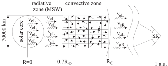
FIG. 1.: Geometry of neutrino trajectories in random magnetic fields. The finite radius of $\nu_{eL}$-neutrino source, the solar core radius $0.1R_{\odot}$ is shown.

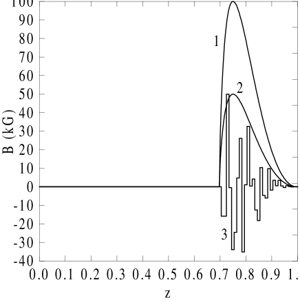
FIG. 2.: Profiles of regular and random magnetic fields in the solar convective zone. One realization of random magnetic field component $b_{x}(r)$ (for one neutrino ray) is plotted. $b_{y}(r)$ component which has a different profile is not shown. 1 - regular magnetic field profile with $B_{max}=100~{}kG$, 2 - the same with $B_{max}=50~{}kG$, 3 - random magnetic field profile with $b_{rms}=50~{}kG$.

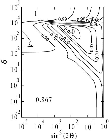
FIG. 3.: The averaged (over 50 rays) survival probability $P_{ee}=\langle\nu_{eL}^{*}\nu_{eL}\rangle$ in dependence on $\delta=\Delta m^{2}/4E=8.81\times 10^{8}~{}\Delta m^{2}(eV^{2})/E(MeV)$ and $\sin^{2}2\theta$ – parameters for $b_{r.m.s.}=50~{}kG$ and correlation length $L_{0}=10^{4}~{}km$.

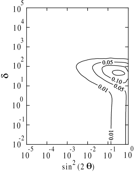
FIG. 4.: As previous figure. The average probability $P_{\bar{e}\bar{e}}=\langle\bar{\nu}_{eR}^{*}\bar{\nu}_{eR}\rangle$.

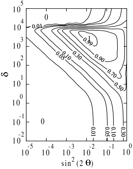
FIG. 5.: As previous figure. The average probability $P_{\mu\mu}=\langle\nu_{\mu L}^{*}\nu_{\mu L}\rangle$.

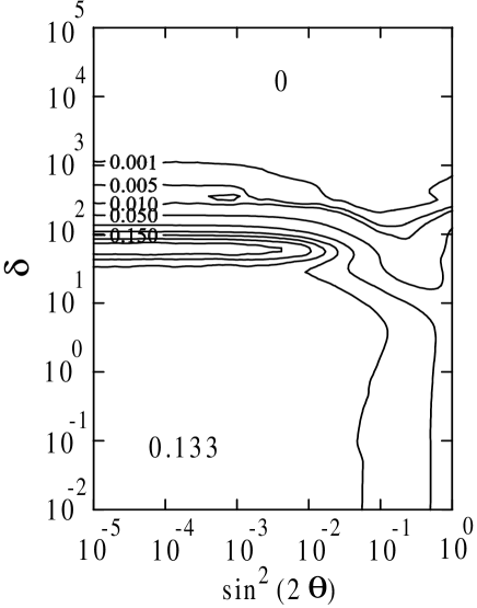
FIG. 6.: As previous figure. The average probability $P_{\bar{\mu}\bar{\mu}}=\langle\bar{\nu}_{\mu R}^{*}\bar{\nu}_{\mu R}\rangle$.

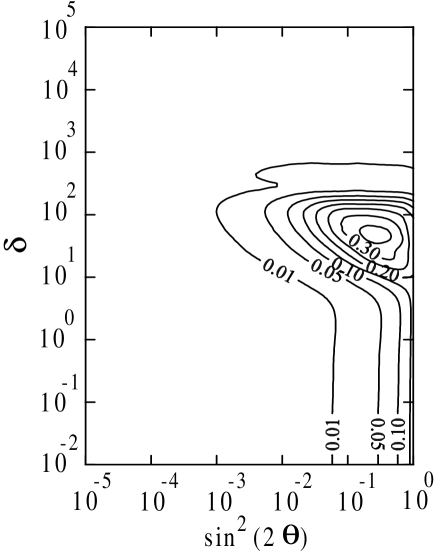
FIG. 7.: As previous figure. The average probability $P_{\bar{e}\bar{e}}=\langle\bar{\nu}_{eR}^{*}\bar{\nu}_{eR}\rangle$ for $b_{r.m.s.}=100~{}kG$ and correlation length $L_{0}=10^{4}~{}km$.

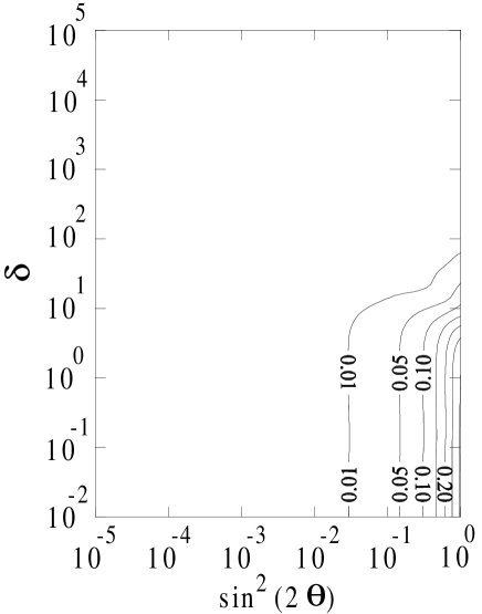
FIG. 8.: The probability $P_{\bar{e}\bar{e}}=\langle\bar{\nu}_{eR}^{*}\bar{\nu}_{eR}\rangle$ in dependence on $\delta=\Delta m^{2}/4E$ and $\sin^{2}2\theta$-parameters for the regular field $B_{0}=50~{}kG$.

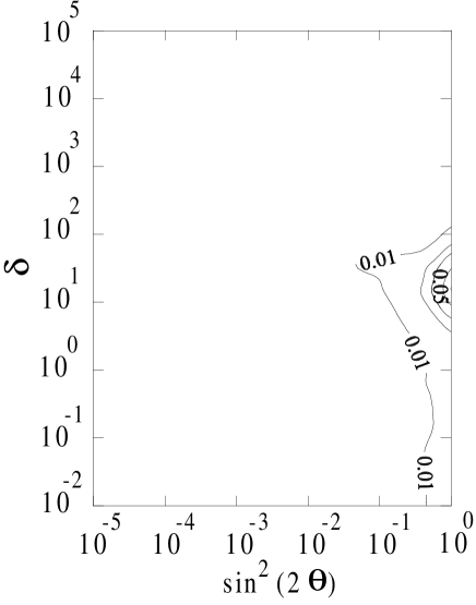
FIG. 9.: As previous figure. The average probability $P_{\bar{e}\bar{e}}=\langle\bar{\nu}_{eR}^{*}\bar{\nu}_{eR}\rangle$ for the regular field $B_{0}=100~{}kG$.

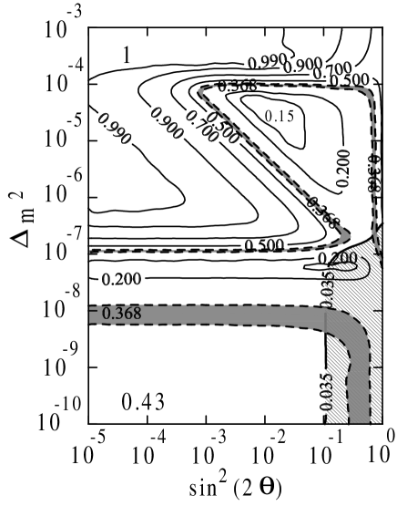
FIG. 10.: $\Delta m^{2}~{}(eV^{2})$, $\sin^{2}2\theta$ -plane for the ratio DATA/SSM in the regular field $B_{0}=50~{}kG$. The isoline $DATA/SSM=0.368\pm 0.026$ allowed from the SK experiment is shown by the dashed line. The SK bound on $\bar{\nu}_{eR}$ Eq. (51) is plotted too separating the excluded area.

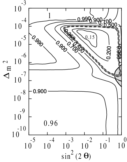
FIG. 11.: As previous figure for the ratio DATA/SSM in the regular field $B_{0}=100~{}kG$.

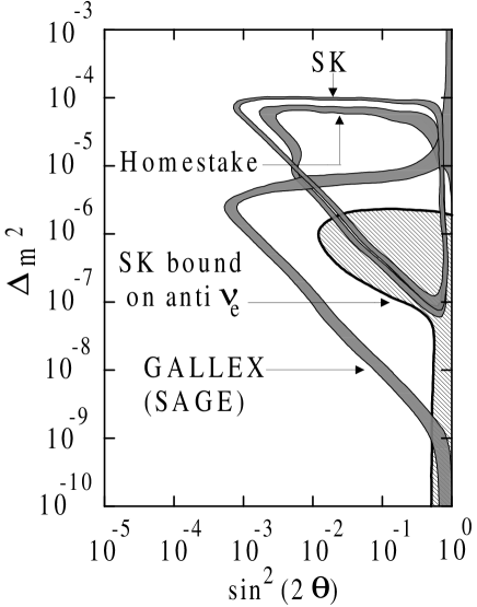
FIG. 12.: The reconcilement of all experiments. The isolines with dashed bands represent the DATA/SSM ratio equal correspondingly to $0.368\pm 0.026~{}$(SK), $0.509\pm 0.059$, $0.504\pm 0.085$ (GALLEX+SAGE), and $0.274\pm 0.027~{}$(Homestake). The random field $b_{rms}=50~{}kG$ and correlation length $L_{0}=10^{4}~{}km$.

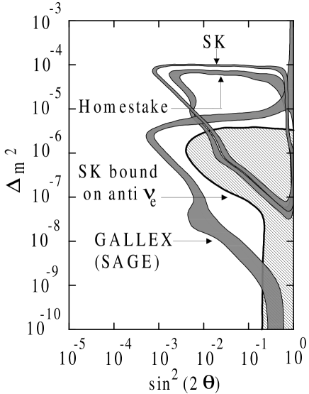
FIG. 13.: As previous figure. The random field $b_{rms}=100~{}kG$ and correlation length $L_{0}=10^{4}~{}km$.

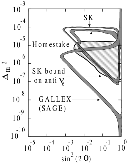
FIG. 14.: As previous figure. The random field $b_{rms}=100~{}kG$ and correlation length $L_{0}=10^{3}~{}km$.

REFERENCES

• [1] Y. Suzuki, Rapporter talk at 25th ICRC (Durban) 1997.
• [2] V. Berezinsky, astro-ph/9710126, invited lecture at 25th International Cosmic Ray Conference, Durban, 28 July - 8 August, 1997.
• [3] E.N. Parker, Astrophys. J., 408 (1993) 707;
E.N. Parker, Cosmological Magnetic Fields, Oxford University Press, Oxford, 1979.
• [4] S.I. Vainstein, A.M. Bykov, I.M. Toptygin, Turbulence, Current Sheets and Shocks in Cosmic Plasma, Gordon and Breach, 1993.
• [5] A.Nicolaidis,Phys.Lett., B262 (1991) 303.
• [6] K. Enqvist, P. Olesen, V.B. Semikoz, Phys. Rev. Lett. 69 (1992) 2157
K.Enqvist, A.I. Rez, V.B. Semikoz, Nucl. Phys. B436 (1995) 49;
S. Pastor, V.B. Semikoz, J.W.F. Valle, Phys. Lett. B369 (1996) 301.
• [7] E. Kh. Akhmedov, Phys. Lett. B 213 (1988) 64;
C.-S. Lim and W.J. Marciano, Phys. Rev. D 37 (1988) 1368.
• [8] E.Kh. Akhmedov, β€œThe neutrino magnetic moment and time variations of the solar neutrino flux”, Preprint IC/97/49, Invited talk given at the 4-th International Solar Neutrino Conference, Heidelberg, Germany, April 8-11, 1997.
• [9] G. Fiorentini, M. Moretti and F.L. Villante, hep-ph/9707097
• [10] E.Kh. Akhmedov, S.T. Petcov and A.Yu. Smirnov, Phys. Rev. D48 (1993) 2167; Phys. Lett. B309 (1993) 95.
• [11] S. Pastor, V.B. Semikoz and J.W.F. Valle, Phys. Lett. B423 (1998) 118; hep-ph/9711316
• [12] A.B. Balantekin and F. Loreti, Phys. Rev. D48 (1993) 5496.
• [13] John N. Bahcall, Neutrino Astrophysics, Cambridge University Press, 1988, section 6.3.
• [14] I.M.Lifshitz, S.A.Gredeskul, and L.A.Pastur, Sov. Phys. JETF 83 (1982) 2362 (in Russian).
• [15] V.B. Semikoz, Nucl.Phys. B501 (1997) 17
• [16] J.K. Rowley et al. in Solar Neutrinos and Neutrino Astronomy, AIP Conference Proceedings, 126, edited by M.L. Cherry, W.A. Fowler and K. Lande, (1985);
Β P.Anselman et al. Phys. Lett. B327 (1994) 377;
J.N.Abdurashitov et al. Phys.Lett. B328 (1994) 234.
• [17] Status Report of Borexino Project: The Counting Test Facility and its Results. A proposal for participation in the Borexino Solar Neutrino Experiment, J.B. Benziger et al., (Princeton, October 1996). Talk presented by P.A. Eisenstein at Baksan International School ” Particles and Cosmology” (April 1997).
• [18] F. Arzarello et al. Preprint CERN-LAA/94-19, College de France LPC/94-28;
C. Laurenti et al. Proceedings of the 5th Int. Workshop on Neutrino Telescopes, Venice XXX;
G. Bonvicini, Nucl. Phys. B (Proc. Suppl.) 35 (1994) 438.
• [19] J.N. Bahcall, M.H. Pinsonneault, Rev. Mod. Phys. 67 (1995) 781.
• [20] W.Grimus and T. Scharnagl, Mod. Phys. Lett. A8 (1993) 1943
• [21] Ya.A. Zeldovich, A.A. Ruzmaikin, D.D. Sokoloff, Magnetic fields in astrophysics, Cordon and Breach, N.Y., 1983
• [22] A.A. Ruzmaikin, A.M. Shukurov, D.D. Sokoloff, Magnetic fields of Galaxies, Kluwer, Dordrecht, 1988.
• [23] S.I. Vainstein, F. Cattaneo, 1992, Astrophysical Journal, 393 (1992) 165.
• [24] A.V. Gruzinov, P.H. Diamond, 1994, Phys. Rev. Lett., 72 (1994) 1651.
• [25] A.A. Abrikosov, L.P. Gorkov, I.E. Dzyaloshinski, Methods of Quantum Field in Statistical Physics, Prentice Hall, 1963.
• [26] A.B.Balantekin, J.M.Fetter, and F.N.Loreti, Phys. Rev. D 54 (1996) 3941.
• [27] G.G. Likhachev, A.I. Studenikin, Sov. Phys. JETP, 81 (1995) 419.
• [28] J.N. Bahcall, P. Krastev, Preprint IASSNS-AST 97/31.
• [29] J. Schechter, J.W.F. Valle, Phys. Rev. D 24 (1981) 1883; Err. Phys. Rev. D 25 (1982) 283.
• [30] I.R. Barabanov et al., Astroparticle Phys., 5 (1996) 159.
Refer to caption