On the evolution of abelian-Higgs string networks

Abstract

We study the evolution of abelian-Higgs string networks in numerical simulations. These are compared against a modified velocity-dependent one scale model for cosmic string network evolution. This incorporates the contributions of loop production, massive radiation and friction to the energy loss processes that are required for scaling evolution. We find that the loop distribution statistics in the simulations are consistent with the long-time scaling of the network being dominated by loop production. For an oscillating sinusoidal perturbation, we also demonstrate that the power emitted into massive radiation decays strongly with wavelength. Putting these observations together and extrapolating, we believe there is insufficient evidence to reject the the standard picture of string network evolution in favour of one where direct massive radiation is the dominant decay mechanism, a proposal which has attracted much recent interest.

1 Introduction

Vortex-string networks are important in a variety of contexts, whether in condensed matter physics or cosmology[1]. If we are to obtain a quantitative description of these networks, then we must also properly understand their ‘scaling’ evolution as well as the decay mechanisms which maintain it. The abelian-Higgs model, a relativistic version of the Ginzburg-Landau theory of superconductors, provides a convenient testbed for developing detailed models for this evolution. On the one hand, the relatively simple field theory can be studied directly in three-dimensional simulations. On the other, a straightforward reduction to a one-dimensional effective theory—the Nambu action—can also be studied numerically, though over a much wider dynamic range.

In a cosmological context, a rather simple ‘one-scale’ model of string evolution has emerged[2, 3] which appears to successfully describe the large-scale features of an evolving string network[4, 5], though with subtleties remaining on smaller scales. In this simple model, the average number of long strings in a horizon volume remains fixed as it expands, a rapid dilution made possible through reconnections resulting in loop production. The loops, in this standard picture, oscillate relativistically and decay through gravitational radiation. The subtlety here concerns small loop creation; gravitational radiation backreaction effects should act on the long string network eliminating small wavelength modes, thus setting a minimum loop creation size[4, 6]. This backreaction length ‘scales’ with the horizon size (for GUT-scale strings it should be approximately $10^{-4}t$), and so loop sizes should also be scale-invariant, albeit tiny and, as yet, not adequately probed by Nambu string simulations.

Recently this standard picture for network evolution has been questioned on the basis of abelian-Higgs field theory simulations[7]. The authors suggest that the primary energy loss mechanism by long strings is direct massive radiation, rather than loop creation. This is contrary to qualitative expectations that the presence of a large mass threshold should exponentially suppress massive particle production for any long wavelength oscillatory string modes, that is, those much larger than the string width[8]. Evidence in support of this claim rests primarily on the study of large amplitude oscillations of a single string and network simulations in which the loop density is observed to be low.

The aim of the present work is to consider these issues by taking a more detailed look at radiation from an oscillating string and the available decay mechanisms for an evolving network. In high resolution and low noise simulations of a perturbed string, we are able first to demonstrate that qualitative expectations for massive radiation suppression are correct. Next, by analytically modelling the small-scale results from field theory network simulations, we are able to argue that these can be sensibly and consistently extrapolated to the large lengthscales relevant for Nambu simulations and cosmology. Although complex nonlinear processes are at work on small-scales in the field theory simulations, loop and ‘protoloop’ production already appears to be the be the dominant energy decay mechanism.

2 Massive radiation from an oscillating string

As stated above, we shall be considering strings in the Abelian Higgs model, the simplest producing gauged vortex-lines. The Lagrangian density is

$${\mathcal{L}}=(D_{\mu}\phi)^{*}(D^{\mu}\phi)-\frac{1}{4}F_{\mu\nu}F^{\mu\nu}-\frac{\lambda}{4}(\phi\phi^{*}-\eta^{2})^{2}.$$ (1)

The covariant derivative $D_{\mu}$ acts on $\phi$ as $\partial_{\mu}-ieA_{\mu}$. The Higgs field mass is $\sqrt{\lambda}\eta$ and that of the vector field is $\sqrt{2}e\eta$. After rescaling the only free parameter in the model is the ratio of these two masses, which we take to be unity (specifically, $\lambda/2=\eta=e=1$). This corresponds to the Bogomol’nyi limit for vortices in two dimensions. The system of evolution equations resulting from ((1)) is solved using the standard lattice gauge theory methods proposed by Myers et al. [9] (we also always adopt the temporal gauge $A_{0}=0$). Initial data is evolved forward in time using a leap-frog discretization of Hamilton’s equations with a short time-step. Throughout our simulations the boundary conditions in use are periodic up to a gauge transformation in all cases and exactly periodic for network simulations.

First, we consider a perturbed string lying in the $z$-direction and oscillating in a periodic box of sidelength $L$. The starting configuration for each simulation is based on a simple ansatz for which the core position varies sinusoidally along the string length with amplitude $y=A\sin(2\pi z/L)$. We use profile functions obtained by solving the one dimensional field equations for a cylindrical string numerically. If, as we suggest, the perturbed string is weakly radiating for large $L$ then it is necessary to distinguish the ’true’ radiation from that due to the spurious modes introduced by inappropriate initial conditions. We achieve this by relaxing the gauge links in our lattice system to their energetic minimum, while fixing the Higgs field, and hence the position of the string core (this removes the worst modes). Further spurious modes associatied with the Higgs field modulus are then removed by a releasing all the fields for a short period to evolve via ‘gradient flow’, that is, purely first-order dissipative evolution.

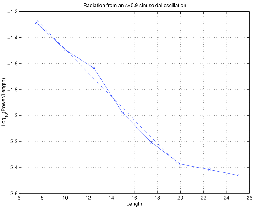
Figure 1: The power per unit length emitted by a oscillating strings as a function of length $L$, initially given a fixed relative amplitude $\epsilon=2\pi A/L=0.9$. The fall-off with increasing length is not consistent with the $L^{-1}$ required for scaling. The dashed line is a best least-squares fit to exponential fall-off.

To calculate radiative power we look at the rate of change of energy outside a region of fixed radius around the position of the unperturbed string. We take the average initial energy increase as the radiation rate and the effect of varying the string length is illustrated in Figure 1. Here, the relative amplitude for the initial data was kept at a large fixed value, $\epsilon\equiv 2\pi A/L=0.9$; it is important that this value is below unity because, for $\epsilon\mathrel{\hbox to0.0pt{\lower 4.0pt\hbox{\hskip 1.0pt$\sim$}\hss}\raise 1.0pt\hbox{$>$}}1.0$, the perturbed strings correspond to degenerate relativistic Nambu configurations which radiate pathologically [10]. An exponential trend as a function of length $L$ is apparent, which can be approximately fitted by $P\propto\exp(-L/L_{\rm m})$ with $L_{\rm m}\approx 4.8$. For smaller amplitude, there is an even stronger dependence on $L$, so we can be confident that $L_{\rm m}\mathrel{\hbox to0.0pt{\lower 4.0pt\hbox{\hskip 1.0pt$\sim$}\hss}\raise 1.0pt\hbox{$<$}}4.8$ for $\epsilon\mathrel{\hbox to0.0pt{\lower 4.0pt\hbox{\hskip 1.0pt$\sim$}\hss}\raise 1.0pt\hbox{$<$}}0.9$ (as we describe in more detail elsewhere [11]). Certainly the decay of emitted power between the shortest and longest $L$ shown here is consistent only with a higher power law than is required for scaling, that is, $P\propto L^{-n}$ with $n>\!>1$. For $L$ significantly larger than shown in Figure 1, the minute power loss becomes indistinguishable from the background numerical noise inherent in the simulations. Note that the actual spectral nature of this radiation and its relationship to the string perturbation lengthscale $L$ is discussed at length elsewhere [11].

The strong scale-dependence of massive radiation we observe is not consistent with the behaviour found in ref. [7], where they suggest that the power per unit length scales merely as $P\propto L^{-1}$. We can see two possible explanations for this clear discrepancy: First, the results reported in ref. [7] are for only a single relative perturbation amplitude $\epsilon=\pi$. This is a strongly nonlinear and degenerate regime for which pathologically strong radiation is expected. Secondly, for large amplitudes the unrelaxed initial ansatz in ref. [7] is inaccurate, particularly for the gauge fields. As we have observed in our own simulations, this can lead to spurious modes from the initial relaxation which swamp the radiation due to the string oscillations.

3 String network evolution

We have performed network simulations using periodic cubic lattices of side length 250 and greater. The principal physical parameter in each simulation is the initial correlation length. To establish a suitable network configuration we take an initial configuration with a flat initial power spectrum of fluctuations in the Higgs field, centered around zero, and zero gauge field. This is evolved forward in time with Hamiltonian dynamics to increase the correlation length and then acted upon by a short period of gradient flow evolution to reduce the initial inter-string energy density to a negligible value, since the one-scale model requires that this be zero initially. Subsequently the simulation is evolved using Hamiltonian dynamics. The Gauss constraint is satisfied initially as we start from rest, and is preserved by the equations of motion.

The time-step is chosen to be sufficiently small to allow the Hamiltonian to be conserved within 1 per cent over the course of a run. The choice of spatial lattice spacing is constrained by the desire to meet two conflicting criteria: (i) to simulate a volume which is orders of magnitude larger than the string width, and (ii) to accurately represent the continuum theory. Throughout we have chosen a lattice size of 0.5, which is as large as we feel is reasonable given that at larger spacings there is a significant potential barrier associated with the lattice and that for oscillating strings of length $\approx 15$ we have observed greatly increased radiation using a larger lattice spacing.

To characterise the network configuration at a given point in time we assign positions of zeros of the Higgs field to lattice plaquettes according to the winding of the Higgs phase around each plaquette. This allows us to calculate correlation lengths and loop distribution statistics [5]. When combined with similar data from a nearby time-step we can also estimate the velocity of each string segment. The procedure for calculating velocities is relatively vulnerable to numerical errors due to uncertainty in the ‘true’ position of the string network and the sensitivity of measured velocities to this.

In Figure 2 we see general consistency with the results of Figure 1 of Vincent et al. . In both cases the network correlation length grows approximately linearly throughout the simulations. The most notable deviations from linearity is seen in the run at largest lattice spacings of ref. [7], where the rate of growth of the correlation length with time is $\sim 0.5$, some 50 per cent greater than in the rest of the simulations. We speculate that this increased rate of growth is caused by lattice effects. The initial brief burst of growth in correlation length seen by Vincent et al. in several simulations is not seen in our simulations and may arise from the slightly different procedures used to set up the initial network configurations.

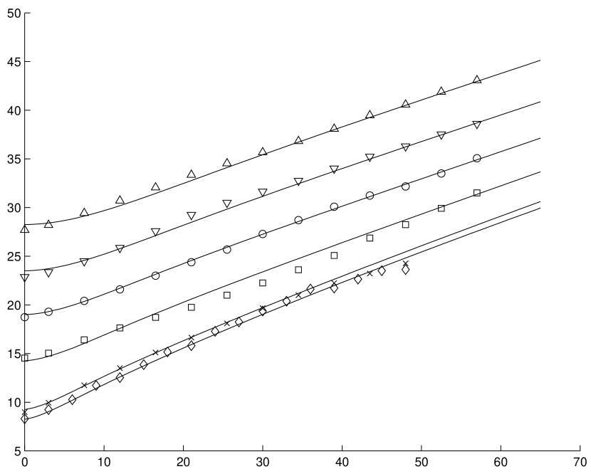
Figure 2: The spatial correlation length $L$ as a function of time for a series of simulations with a grid size of $250^{3}$. A velocity dependent ‘one-scale’ model is used to fit the data (solid lines).

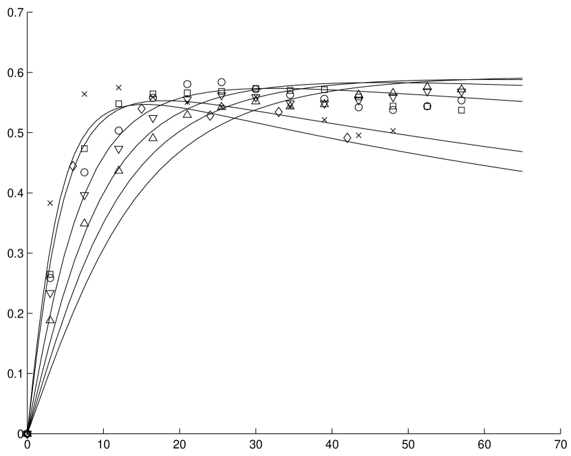
Figure 3: The average rms velocity $v$ as a function of time for a series of simulations with a grid size of $250^{3}$. The solid lines indicate the fit of our simple analytic model.

4 Analytic modelling of network evolution

If we regard the one-dimensional Nambu action as providing a satisfactory first approximation to string evolution then we can employ a velocity-dependent ‘one-scale’ model to describe the evolution of a string network [3]. The long string network energy density $\rho_{\infty}$ is susceptible to three possible energy loss mechanisms, friction, loop production and direct massive radiation which are phenomenologically summarized in the following averaged evolution equation [3]:

$$\frac{d\rho_{\infty}}{dt}=\frac{v^{2}\rho_{\infty}}{L_{\rm f}}+\frac{\bar{c}v\rho_{\infty}}{L}+{\rho_{\infty}}f({L}/{L_{\rm m}})\,,$$ (2)

where $L_{f}$ is the friction length, $\bar{c}$ is the loop chopping efficiency, and $f({L}/{L_{\rm m}})$ is proportional to the power per unit length of massive radiation. Employing the definition for the correlation length $\rho_{\infty}\equiv\mu/L^{2}$ and noting a supplementary equation for the rms velocity $v$ we obtain [3]

$$\frac{dL}{dt}=\frac{Lv^{2}}{2L_{\rm f}}+\frac{\bar{c}v}{2}+\frac{L}{2}f({L}/{L_{\rm m}})\,,$$ (3)

$$\frac{dv}{dt}=(1-v^{2})\left[\frac{1-2v^{2}}{L}-\frac{v}{L_{\rm f}}-a\frac{2\bar{c}v^{2}}{L}\right]\,.$$ (4)

We provide some explanation for the origin of these terms below, but note that the first term in the velocity equation is due to the acceleration of strings with a typical curvature radius $L$ (with $v\rightarrow 1/\sqrt{2}$ for free relativistic motion). Given the difficulties in measuring and normalizing this velocity in the field theory simulations, we also allow for lattice discretization effects through the phenomenological parameter $a$; this term takes a form which could also incorporate momentum losses due to loop production.

A potentially important energy loss mechanism for the string network is friction through interactions with background energy density $\bar{\rho}$. For the simulations described here with dissipative initial conditions, this background arises dynamically through the decay of the string network into massive particles, that is, $\bar{\rho}=\rho_{\infty,\rm i}-\rho_{\infty}$. Characterising this in terms of a friction lengthscale above which friction dominates, we have $L_{\rm f}\equiv\mu\beta/{\bar{\rho}}=\beta(1/L_{\rm i}^{2}-1/L^{2})^{-1}$ (for $L\rightarrow\infty$ in flat space, $L_{\rm f}\rightarrow\beta L_{\rm i}^{2}$. We can bound the friction coefficient $\beta$ by beginning with a high density string network and assuming a late-time friction-dominated regime. An example is the lowest curve in Figure 2, where friction affects the scaling behaviour, most obviously through the velocity in Figure 3; this provides a lower limit of $\beta\mathrel{\hbox to0.0pt{\lower 4.0pt\hbox{\hskip 1.0pt$\sim$}\hss}\raise 1.0pt\hbox{$>$}}0.2$. From this we can infer that friction provides less than 10% of the energy losses for the duration of the simulations in Figure 2, if the initial correlation length satisfies $L_{\rm i}\mathrel{\hbox to0.0pt{\lower 4.0pt\hbox{\hskip 1.0pt$\sim$}\hss}\raise 1.0pt\hbox{$>$}}20$. Hence, assuming friction to be insignificant for the lowest density simulations, we can make a more accurate estimate $\beta\approx 0.3$.

Loop production is caused by the intersections and self-intersections of long strings. For the simulations least affected by friction, let us assume the standard picture with energy losses predominantly due to this loop production. In this case, from a fit to the correlation length and velocities we can obtain the asymptotic value $\bar{c}\approx 0.75$ (with some small momentum losses $a\approx 0.45$). This value of $\bar{c}$ is consistent with previous determinations of the loop chopping efficiency in flat space simulations [12]; note that the velocity-dependence in our definition implies that their $c=\bar{c}/v$).

Direct massive radiation will provide some energy losses in the early evolution, but this should diminish as the correlation length increases, consistent with the behaviour of the oscillating string discussed in section 2. From Figure 2 we can see that there is considerable evidence for an additional scale-dependent initial energy loss mechanism, since the initial slopes for the smaller correlation lengths are clearly steeper than those with $L_{\rm i}\mathrel{\hbox to0.0pt{\lower 4.0pt\hbox{\hskip 1.0pt$\sim$}\hss}\raise 1.0pt\hbox{$>$}}15$. From a fit to Figure 2, the function describing the energy losses into massive radiation should behave approximately as $f(L/L_{\rm m})\approx\gamma\exp(-L/L_{\rm m})$ with $L_{\rm m}\sim 4.8$ for the present parameters. The overall strength $\gamma$ can only be rougly estimated from the initial slopes in Figure 2 to yield $\gamma\sim 0.15$. This implies, consistent with Figure 2, that massive radiation provides a strong initial contribution only for $L\mathrel{\hbox to0.0pt{\lower 4.0pt\hbox{\hskip 1.0pt$\sim$}\hss}\raise 1.0pt\hbox{$<$}}10$ and, subsequently, it is rapidly curtailed.

What we obtain finally is the self-consistent fit of our analytic model to the correlation length and velocity evolution shown in Figure 2. Asymptotically this is quantitatively in agreement with the standard picture of long string evolution, and it also reproduces predicted qualitative features. However, if we choose to ignore the loop contribution as in ref. [7] and we assume that massive radiation losses are scale-invariant ($f\propto L^{-1}$), then it is also possible to fit the asymptotic data with this analytic model, although the initial qualitative features would not be as consistent. The question of whether the dominant loop loss interpretation is correct, therefore, must hinge on more precise information about the loop distribution and how it evolves in time.

5 Competing energy loss mechanisms

In using these simulations to determine the dominant decay mechanisms for a cosmic string network we face a rather obvious difficulty. If the standard cosmological picture of loop production is correct, then we know from high resolution Nambu string simulations that the typical loop creation scale $\bar{\ell}$ relative to the horizon is $\alpha\equiv\bar{\ell}/t\mathrel{\hbox to0.0pt{\lower 4.0pt\hbox{\hskip 1.0pt$\sim$}\hss}\raise 1.0pt\hbox{$<$}}10^{-3}$, while radiation backreaction estimates suggest that $\alpha\sim 10^{-4}$ for GUT-scale strings. The present field theory simulations, however, have a dynamic range which is at least two orders of magnitude poorer, so we cannot realistically hope to probe these small-scale regimes. In consequence, we might be surprised to be able to identify any loops at all and we certainly cannot expect their average creation size $\bar{\ell}$ to ‘scale’ relative to $L$. As we observe numerically, most loops which are created have radii comparable to the string thickness, with $\bar{\ell}\sim\pi$ almost constant throughout. Indeed, simulation visualisations indicate that most energy is lost via ‘protoloops’, that is, small-scale highly nonlinear, but coherent, regions of energy density (as illustrated in Figure 4). Consistent with the Nambu simulations, this ‘protoloop’ production occurs—like small loop formation—in high curvature regions where the strings collapse and become very convoluted [13].

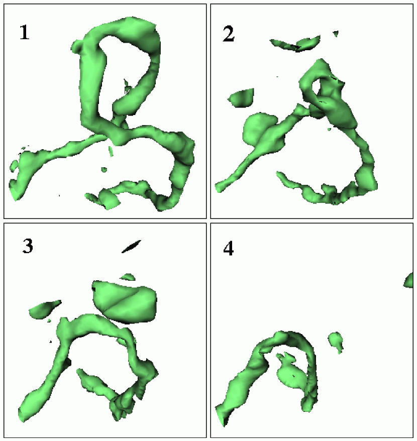
Figure 4: Four stages of the formation of ‘protoloops’ in the field theory simulations. : A highly curved region of string (i) collapses to form nonlinear ‘lumps’ in the energy density (ii) which are lost (iii,iv) when the the string’s topological winding intercommutes or annihilates in this region. Energy density contours are plotted.

A proportion of these ‘protoloops’ have sufficient topology to be identified as loops by our numerical diagnostics, so we can estimate the energy loss via this pathway relative to other mechanisms. Because of dynamic range limitations, all small loop trajectories in these simulations are self-intersecting and loops decay almost as fast as allowed by causality. Their time-dependent length, therefore, can be given by $\ell\approx\ell_{\rm c}-4(t-t_{\rm c})$ in the range $0<t-t_{\rm c}<\ell_{\rm c/4}$ with the loop creation length $\ell_{\rm c}$ and time $t_{\rm c}$. Hence, at any one time, the string energy loss through loop decay can be simply approximated by $\dot{\rho}_{\ell}\approx-4\mu n_{\ell}$, where $n_{\ell}$ is the loop number density. For linear scaling to pertain, a dominant energy loss mechanism must behave as $\dot{\rho}\propto t^{-3}$, implying $n\propto t^{-3}$ so the loop energy density would behave as $\rho_{\ell}=\mu\bar{\ell}n_{\ell}\propto\rho_{\infty}/t$ (with $\bar{\ell}$ constant). Thus, contrary to one of the conclusions in ref. [7], loops can be an important decay mechanism even though their relative contribution to the total string energy density is falling rapidly as $t^{-1}$.

Figure 5 illustrates the relative small loop contribution to the overall energy density losses throughout the particular simulation beginning with $L_{\rm i}=15$. This is compared with the estimated analytic fit for friction, loop losses and massive radiation. We can observe that the measured loop energy losses grow steadily towards the analytic loop contribution, which for these simulations we assume must include ‘protoloops’ both with topology and without it. We can see that the proportion of loops—the topological ‘protoloops’—gradually grows to meet or even overtake the analytic loop contribution by the end of the simulation. In fact our analytic calculation deserves closer quantitative scrutiny because it is a significant overestimate; the histogram plotted in Figure 5 only gives $\mu n_{\ell}L^{3}$ rather than four times this quantity.

With this clear qualitative trend evident, it is not unreasonable to conjecture that an extrapolation by another twenty orders of magnitude to cosmological scales will imply that the loop contribution will be completely dominant. As the typical string perturbation lengthscale grows and is affected by radiative backreaction, it is again reasonable to suppose that the typical loop creation size will also grow, becoming many orders of magnitude larger than the string thickness. We conclude that these field theory simulations, once we account for their small dynamic range, are consistent with the standard picture of long string network evolution via small loop production. At the very least, the simulations do not provide compelling evidence that cosmological strings will decay primarily through the direct radiation of ultra-massive particles.

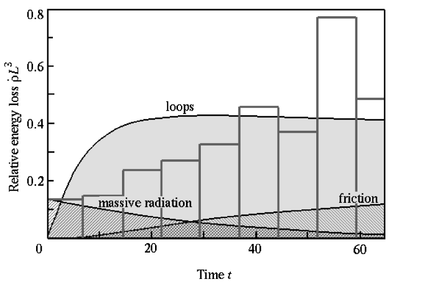
Figure 5: The relative contributions of the different components to the overall energy density losses of the string network, as predicted by the analytic model for the simulation in Figure 2 with $L_{\rm i}=15$. Superposed onto this figure is a histogram of energy loss into loop production estimated directly from measurements of the time-varying loop density in this particular simulation. It is apparent that the loop energy loss contribution is becoming more important as the simulation progresses.

6 Conclusion

We conclude from these numerical results and their analytic interpretation that the standard picture provides a more coherent and adequate model for string network evolution than the more radical alternative based on direct massive radiation[7]. However, this is not to suggest that we have provided a complete or detailed description of the complex nonlinear processes that underlie network evolution on these small scales. Rather, first, we have shown qualitatively that loop production is important for network evolution and should become more so when extrapolated to large scales. Secondly, we have also demonstrated that massive radiation is strongly suppressed for long wavelength modes, implying that it is an inadequate decay channel for maintaining network ‘scaling’. We are currently investigating both these aspects in more quantitative detail[11].

These results have significant cosmological implications. Our expectation is that massive particles will only be produced infrequently in highly nonlinear string regions, such as at cusps and reconnections. The ensuing flux of cosmic rays should be relatively low[14, 15]. The more recent estimates of the ensuing cosmic ray flux from direct massive radiation from strings appear to be overly optimistic[7, 16]. This work points to the need for caution in making cosmological extrapolations from small-scale numerical simulations and to the need for further progress understanding string radiation backreaction.

References

- [1] For a review see A. Vilenkin & E.P.S. Shellard, Cosmic strings and other topological defects (Cambridge University Press, 1994).
- [2] T.W.B. Kibble, Nucl. Phys. B252, 227 (1985). Erratum: Nucl. Phys. B261, 750.
- [3] C.J.A.P. Martins & E.P.S. Shellard, Phys. Rev. D54, 2535 (1996).
- [4] D.P. Bennett & F.R. Bouchet, Phys. Rev. D40, 2408 (1990).
- [5] B. Allen & E.P.S. Shellard, Phys. Rev. Lett. 64, 119 (1990).
- [6] See, for example, D. Austin, E.J. Copeland, & T.W.B. Kibble, Phys. Rev. D48, 5594 (1993).
- [7] G. Vincent, N.D. Antunes, & M.B. Hindmarsh, Phys. Rev. Lett. 80, 908 (1997).
- [8] M.K. Srednicki & S. Thiesen, Phys. Lett. 189B, 397 (1987).
- [9] K.J.M. Moriarty, E. Myers, & C. Rebbi, Phys. Lett. 207B, 411 (1988).
- [10] R.A. Battye & E.P.S. Shellard, Nucl. Phys. B423, 260 (1994).
- [11] J.N. Moore & E.P.S. Shellard [1998], DAMTP preprint. C.J.A.P. Martins, J.N. Moore & E.P.S. Shellard [1998], in preparation.
- [12] G. Vincent, M.B. Hindmarsh & M. Sakellariadou, Phys. Rev. D56, 637 (1997).
- [13] E.P.S. Shellard & B. Allen [1989], ‘On the evolution of cosmic strings’, in The formation and evolution of cosmic strings, G.W. Gibbons, S.W.& Hawking, & T. Vachaspati, eds. (Cambridge University Press). Cambridge, UK
- [14] P. Bhattacharjee, & N.C. Rana, Phys. Lett. 246B, 365 (1990).
- [15] R.J. Protheroe & T. Stanev, Phys. Rev. Lett. 77, 3708 (1996); Erratum-ibid. 78, 3420.
- [16] P. Bhattacharjee, Phys. Rev. Lett. 81, 260 (1998).