MSSM Higgs Boson Phenomenology at the Tevatron Collider

Abstract

The Higgs sector of the minimal supersymmetric standard model (MSSM) consists of five physical Higgs bosons, which offer a variety of channels for their experimental search. The present study aims to further our understanding of the Tevatron reach for MSSM Higgs bosons, addressing relevant theoretical issues related to the SUSY parameter space, with special emphasis on the radiative corrections to the down–quark and lepton couplings to the Higgs bosons for large $\tan\beta$. We performed a computation of the signal and backgrounds for the production processes $W\phi$ and $b\bar{b}\phi$ at the upgraded Tevatron, with $\phi$ being the neutral MSSM Higgs bosons. Detailed experimental information and further higher order calculations are demanded to confirm/refine these predictions.

I Introduction

The precision electroweak measurements performed at LEP, SLD and the Tevatron are consistent with the predictions of the standard model containing a light Higgs boson, with mass of the order of the $Z$ boson mass. The searches for such a Higgs particle continue at the LEP and the Tevatron colliders. The searches at LEP2 ($\sqrt{s}\stackrel{{\scriptstyle<}}{{{}_{\sim}}}200$ GeV) are constrained by the collider energy, and a Higgs boson with standard model–like properties can be found only if its mass is below 105 GeV [4].

The potential for discovering a light Higgs boson at the Tevatron collider when it is produced in association with a $W$ or $Z$ gauge boson has been discussed in several studies [5, 6, 7, 8, 9]. Although the kinematic reach of the Tevatron collider is much greater than for LEP2, the backgrounds to Higgs boson searches at hadron colliders are much larger than in $e^{+}e^{-}$ machines. For this reason, large integrated luminosity is essential to establish a signal at the Tevatron. Within the standard model, the general conclusion is that Run II, with a total integrated luminosity of about 2 fb^-1 per detector, will be unable to extend the Higgs boson mass reach of LEP2. The main questions are: what is the theoretical motivation for a Higgs boson with a mass slightly above the LEP2 reach, and what is the necessary upgrade in luminosity to cover that region?

We address the theoretical motivation by appealing to the minimal supersymmetric extension of the standard model (MSSM). The MSSM has the remarkable property that, for a sufficiently heavy supersymmetric spectrum, it fits to the precision electroweak observables as well as the standard model[10]. Moreover, the lightest CP–even Higgs boson mass $m_{h}$ is constrained to satisfy $m_{h}\stackrel{{\scriptstyle<}}{{{}_{\sim}}}130$ GeV[11, 12]. The Higgs sector of this model consists of two Higgs doublets, with two CP–even Higgs bosons, $h$ and $H$, one CP–odd Higgs boson, $A$, and one charged Higgs boson, $H^{\pm}$. This richer spectrum allows for different production and decay processes at LEP and the Tevatron colliders than in the standard model.

In the supersymmetric limit, the neutral components of the two Higgs boson doublets $H_{1}$ and $H_{2}$ couple to down– and up–type quarks, respectively. Lepton fields couple only to the $H_{1}$ Higgs boson. The MSSM, tree–level Yukawa couplings of the down quarks, leptons and up quarks are related to their respective running masses by

$$h_{d} \simeq \frac{m_{d}}{v\cos\beta},\;\;\;\;\;\;\;\;\;\;\;h_{l}\simeq\frac{m_{l}}{v\cos\beta},\;\;\;\;\;\;\;\;\;\;\;h_{u}\simeq\frac{m_{u}}{v\sin\beta},$$ (1)

where $\tan\beta=v_{2}/v_{1}$ is the ratio of the vacuum expectation values of the two Higgs doublets, and $v=\sqrt{v_{1}^{2}+v_{2}^{2}}$=174 GeV. In the standard model, only the top quark Yukawa coupling $h_{t}$ is of order one at the weak scale. In the MSSM, instead, the bottom and $\tau$ Yukawa couplings, $h_{b}$ and $h_{\tau}$, can become of the same order as $h_{t}$, if $\tan\beta$ is sufficiently large. This can have important phenomenological consequences.

Quite generally, the two CP–even Higgs boson eigenstates are a mixture of the real, neutral $H_{1}$ and $H_{2}$ components,

$$\left(\begin{array}[]{c}h\\ H\end{array}\right)=\left(\begin{array}[]{cc}-\sin\alpha&\cos\alpha\\ \cos\alpha&\sin\alpha\end{array}\right)\left(\begin{array}[]{c}H_{1}^{0}\\ H_{2}^{0}\end{array}\right),$$ (8)

and the lightest CP–even Higgs boson couples to down quarks (leptons), and up quarks by its standard model values times $-\sin\alpha/\cos\beta$ and $\cos\alpha/\sin\beta$, respectively. The couplings to the heavier CP–even Higgs boson are given by the standard model values times $\cos\alpha/\cos\beta$ and $\sin\alpha/\sin\beta$, respectively. Analogously, the coupling of the CP–odd Higgs boson to down quarks (leptons) and up quarks is given by the standard model coupling times $\tan\beta$ and $1/\tan\beta$, respectively. Moreover, the lightest (heaviest) CP–even Higgs boson has $ZZh$ and $WWh$ ($ZZH$ and $WWH$) couplings which are given by the Standard Model value times $\sin(\beta-\alpha)$ ($\cos(\beta-\alpha)$), while it can be produced in association with a CP–odd Higgs boson with a $ZhA$ ($ZHA$) coupling which is proportional to $\cos(\beta-\alpha)$ ($\sin(\beta-\alpha)$).

For sufficiently large values of the CP–odd Higgs boson mass $m_{A}$, the effective theory at low energies contains only one Higgs doublet, with standard model–like properties, in the combination

$$h\simeq\phi^{SM}=H_{1}^{0}\cos\beta+H_{2}^{0}\sin\beta;\;\;\;\;\;\;\;<\phi^{SM}>=v\;,$$ (9)

where $\sin\alpha\simeq-\cos\beta$, $\cos\alpha\simeq\sin\beta$ and hence $\sin^{2}(\beta-\alpha)=1$. In this limit, if all supersymmetric particles are heavy, all phenomenological conclusions drawn for a SM Higgs boson are robust when extended to the the lightest CP–even Higgs boson of the MSSM, which, as mentioned before, is at the same time constrained to have a mass below about 130 GeV. For large $\tan\beta$, one of the CP–even neutral Higgs bosons tends to be degenerate in mass with the CP–odd Higgs boson and couples strongly to the bottom quark and tau lepton. The other CP–even Higgs boson has standard model–like couplings to the gauge bosons, while its coupling to the down quarks and leptons may be highly non–standard. If $m_{A}$ is large, then $h$ is the Higgs boson with SM–like properties as described above. If $m_{A}$ is small, then $H$ is the one with SM–like couplings to the gauge bosons. In the following, the symbol $\phi$ denotes a generic Higgs boson.

In this article, we analyze the discovery potential of the Tevatron collider for MSSM Higgs bosons in different production channels. Section 2 discusses the signals from Higgs boson production in association with weak gauge bosons and their dependence on the MSSM parameter space. Section 3 contains details of Yukawa coupling effects for large $\tan\beta$. Section 4 deals with the phenomenological implications of these effects for signals in the $W\phi$ and $b\bar{b}\phi$ production channels. In section 5, we consider the correlation between the bottom mass corrections and the supersymmetric contributions to the branching ratio $B(b\rightarrow s\gamma)$. Finally, section 6 is reserved for our conclusions.

II Signals from $W\phi$ and $Z\phi$ Production

The production of $W\phi$, followed by the decays $W(\to e\nu_{e})$ or $W(\to\mu\nu_{\mu})$ and $\phi(\to b\bar{b})$, is the gold–plated search mode for the standard model Higgs boson $\phi=\phi^{SM}$ at the Tevatron collider, while LEP2 is sensitive to the $Z\phi^{SM}$ process. The production of $Z\phi$ may also be useful at the Tevatron, depending on the efficiency for triggering on missing $E_{T}$ ($\hbox to0.0pt{\hbox to7.95831pt{\hfil/\hfil}\hss}E_{T}$) and the $b\bar{b}$ mass resolution. Additionally, the all–hadronic decays of $W\phi+Z\phi$ may extend the reach, and the Higgs boson decay $\phi(\to\tau^{+}\tau^{-})$ may be observable. However, there are several, unresolved experimental issues concerning these channels that require detailed study by the experimental collaborations. For this reason, at present we shall only consider the $W\phi$ channel at the Tevatron.

To quantify the experimental reach in a model independent way, it is useful to consider the function

$$R=\frac{\sigma(p\bar{p}\to W\phi)}{\sigma(p\bar{p}\to W\phi^{SM})}\frac{B(\phi\to b\bar{b})}{B(\phi^{SM}\to b\bar{b})},$$ (10)

where $\sigma$ denotes a production cross section, $B$ denotes a branching ratio and $\phi^{SM}$ represents a standard model Higgs boson. In the MSSM, the ratio of cross sections is just given by $\sin^{2}(\beta-\alpha)$ or $\cos^{2}(\beta-\alpha)$ depending on $\phi$ being the lightest or heaviest CP–even Higgs, respectively, while the ratio of branching ratios has a more complicated behavior. It is important to notice that, barring the possibility of large next–to–leading–order (NLO), SUSY corrections to the $WW\phi$ vertex, there is no enhancement of the production cross section in the MSSM over the standard model. On the other hand, the branching ratio to $b\bar{b}$ and $\tau^{+}\tau^{-}$ final states are affected by the factors $-\sin\alpha/\cos\beta$ for $h$ and $\cos\alpha/\cos\beta$ for $H$ over the SM Higgs boson couplings to down quarks and leptons. These factors can produce an increase or decrease of the MSSM coupling of the Higgs boson to bottom quarks, depending on the value of the CP–odd mass, $\tan\beta$ and the top and bottom squark mass parameters. In this study, the Higgs boson properties are calculated using the program Hdecay[13].

As mentioned above, for large $m_{A}$, the low–energy, effective theory contains only one Higgs boson with SM–like properties. The Yukawa couplings tend to the standard model values, and $\sin^{2}(\beta-\alpha)\simeq 1$. As long as no new decay modes are open, $h$ has the same properties as $\phi^{SM}$, and a discovery or exclusion limit for a standard model Higgs boson applies equally well to $h$, and $R=1$. If Higgs boson decays to sparticles become important, then it is quite likely that additional Higgs boson production modes exist and enhance the potential signal, rather than decrease it. For example, if the sparticle spectrum is of the order of $m_{h}$, then processes like $p\bar{p}\to N_{2}(\to N_{1}h)C_{1}(\to N_{1}W)+X$ can occur. In our analysis, we shall always consider the limit of heavy sparticle masses, where such supersymmetric contributions to the Higgs production and decay processes are negligible.

In the large $m_{A}$ limit, the renormalization–group improved result for the lightest Higgs boson mass, including two–loop leading–log effects [11, 12, 14, 15], has the approximate analytic form [11]:

$$m_{h}^{2}\equiv m_{\phi^{SM}}^{2} = M_{Z}^{2}\cos^{2}(2\beta)\left(1-{3\over 8\pi^{2}}{m_{t}^{2}\over v^{2}}t\right)$$ (11)

$$+ {3\over 4\pi^{2}}{m_{t}^{4}\over v^{2}}\left[{1\over 2}\widetilde{X}_{t}+t+{1\over 16\pi^{2}}\left({3\over 2}{m_{t}^{2}\over v^{2}}-32\pi\alpha_{3}\right)\left(\widetilde{X}_{t}t+t^{2}\right)\right],$$ (12)

$$\widetilde{X}_{t} = {2\tilde{a}^{2}}\left(1-{\tilde{a}^{2}\over 12}\right),\;\;\;\;\;\;\;\;\tilde{a}=\bar{A}_{t}-\bar{\mu}/\tan\beta,$$ (13)

where $\bar{\mu}=\mu/M_{S}$ and $\bar{A}_{t}=A_{t}/M_{S}$, with $M_{S}^{2}=(m_{\tilde{t}_{2}}^{2}+m_{\tilde{t}_{1}}^{2})/2$, and $t=\log(M_{S}^{2}/m_{t}^{2})$. The above formula is based on an approximation in which the right–handed and left–handed stop supersymmetry breaking parameters are assumed to be close to each other, and hence the stop mass splitting is induced by the mixing parameter $m_{t}\tilde{a}\times M_{S}$. Moreover, this expression is based on an expansion in powers of $m_{t}\tilde{a}/M_{S}$ and is valid only if $\frac{|m_{\tilde{t}_{1}}^{2}-m_{\tilde{t}_{2}}^{2}|}{m_{\tilde{t}_{2}}^{2}+m_{\tilde{t}_{1}}^{2}}<0.5$, where $m_{\tilde{t}_{1}}$ and $m_{\tilde{t}_{2}}$ are the lightest and heaviest stop mass eigenstates. This simplified expression is very useful for understanding the results of this work, although we go beyond this approximation [11] in our full analysis. Finally, in the above, we have ignored corrections induced by the sbottom sector, which, as we shall discuss below, may become relevant for very large values of $\tan\beta$.

The value of $m_{h}$ in Eq. (2.2) is maximized for large values of $\tan\beta$ and $M_{S}$ and $\tilde{a}^{2}=6$. Due to the dependence of the lightest CP–even Higgs mass on $\tan\beta$, LEP will be able to probe the low $\tan\beta$ region of the MSSM. Indeed, recent analyses suggest that even the present, relatively low bounds on a standard model–like Higgs boson from LEP2 have strong implications for the minimal supergravity model [16]. Moreover, it has been shown that, in the large $m_{A}$ region, LEP2 will probe values of $\tan\beta\stackrel{{\scriptstyle<}}{{{}_{\sim}}}2$ for arbitrary values of the stop masses and mixing angles [17]. Since, in general, the lower bound on $\tan\beta$ is expected to be obtained for large values of $m_{A}$, the absence of a Higgs signal in the $ZZh$ channel at LEP2 will provide a strong motivation for models with moderate or large values of $\tan\beta$.

For lower values of the CP–odd Higgs mass, $\sin^{2}(\beta-\alpha)$ can take any value between 0 and 1, and it is a model–dependent question whether $h$ or $H$ produces a viable signal in the $W\phi$ production channel. For moderate or large values of $\tan\beta\stackrel{{\scriptstyle>}}{{{}_{\sim}}}5$, it is easy to identify the main properties of the CP–even Higgs sector. More specifically, three cases may occur:

a) If $m_{A}<m_{\phi^{SM}}$, then $\sin\alpha\simeq-1$, $\cos\alpha\simeq{\cal O}(1/\tan\beta)$ and $\cos(\beta-\alpha)\simeq 1$. In this case, the heaviest CP–even Higgs boson has a production rate which is similar to the standard model case. The branching ratio of the decay into bottom quarks and $\tau$ leptons, however, can become highly non–standard, since $\cos\alpha$ and $\cos\beta$, may differ by a factor of order one.

b) If $m_{A}>m_{\phi^{SM}}$, then the lightest CP–even Higgs boson has a production rate similar to the standard model case. For $m_{A}\gg m_{\phi^{SM}}$, the branching ratio of the decay of this Higgs boson into down quarks is standard model–like. However, when $m_{A}$ becomes close to $m_{\phi^{SM}}$, there can be important differences in the branching ratios with respect to the SM ones.

c) If $m_{A}\simeq m_{\phi^{SM}}$, then $\sin^{2}(\beta-\alpha)\simeq\cos^{2}(\beta-\alpha)\simeq{\cal O}(0.5)$, and the couplings of both neutral CP–even Higgs bosons to bottom quarks tend to be highly non–standard.

To better understand the behavior of the Higgs boson branching ratios in these different cases, we analyze the Higgs boson mass matrix. Assuming the approximate conservation of CP in the Higgs sector, the CP–even Higgs masses may be determined by diagonalizing the 2 $\times$ 2 symmetric mass matrix ${\cal M}^{2}$. After including the dominant one–loop corrections induced by the stop and sbottom sectors, together with the two–loop, leading–logarithm effects, the elements of ${\cal M}^{2}$ are [11]

$${\cal M}^{2}_{11} \simeq m_{A}^{2}\sin^{2}\beta+M_{Z}^{2}\cos^{2}\beta$$ (14)

$$- \frac{h_{t}^{4}v^{2}}{16\pi^{2}}\bar{\mu}^{2}\sin^{2}\beta\tilde{a}^{2}\left[1+\frac{t}{16\pi^{2}}\left(6h_{t}^{2}-2h_{b}^{2}-16g_{3}^{2}\right)\right]+{\cal O}(h_{t}^{2}M_{Z}^{2})$$ (15)

$${\cal M}^{2}_{22} \simeq m_{A}^{2}\cos^{2}\beta+M_{Z}^{2}\sin^{2}\beta\left(1-\frac{3}{8\pi^{2}}h_{t}^{2}t\right)$$ (16)

$$+ \frac{h_{t}^{4}v^{2}}{16\pi^{2}}12\sin^{2}\beta\left\{t\left[1+\frac{t}{16\pi^{2}}\left(1.5h_{t}^{2}+0.5h_{b}^{2}-8g_{3}^{2}\right)\right]\right.$$ (17)

$$+ \left.\bar{A}_{t}\tilde{a}\left(1-{\bar{A}_{t}\tilde{a}\over 12}\right)\left[1+\frac{t}{16\pi^{2}}\left(3h_{t}^{2}+h_{b}^{2}-16g_{3}^{2}\right)\right]\right\}$$ (18)

$$- \frac{v^{2}h_{b}^{4}}{16\pi^{2}}\sin^{2}\beta\bar{\mu}^{4}\left[1+\frac{t}{16\pi^{2}}\left(9h_{b}^{2}-5h_{t}^{2}-16g_{3}^{2}\right)\right]+{\cal O}(h_{t}^{2}M_{Z}^{2})$$ (19)

$${\cal M}^{2}_{12} \simeq -\left[m_{A}^{2}+M_{Z}^{2}-\frac{h_{t}^{4}v^{2}}{8\pi^{2}}\left(3\bar{\mu}^{2}-\bar{\mu}^{2}\bar{A}_{t}^{2}\right)\right]\sin\beta\cos\beta$$ (20)

$$+ \left[\frac{h_{t}^{4}v^{2}}{16\pi^{2}}\sin^{2}\beta\bar{\mu}\tilde{a}\left[\bar{A}_{t}\tilde{a}-6\right]+\frac{3h_{t}^{2}M_{Z}^{2}}{32\pi^{2}}\bar{\mu}\tilde{a}\right]\left[1+\frac{t}{16\pi^{2}}\left(4.5h_{t}^{2}-0.5h_{b}^{2}-16g_{3}^{2}\right)\right],$$ (21)

where $g_{3}$ is the QCD running coupling constant. In the above, we have assumed, for simplicity, that $A_{b}\simeq 0$ (an assumption we shall always make in the following analysis) and retained only the leading terms in powers of $h_{b}$ and $\tan\beta$. We have also included the small, ${\cal O}(h_{t}^{2}M_{Z}^{2})$ correction to ${\cal M}_{12}^{2}$ explicitly because it plays a relevant role in our analysis. The above expressions hold only in the limit of small splittings between the running stop masses. Moreover, the condition $2m_{t}\max(|A_{t}|,|\mu|)<M^{2}_{S}$ must be fulfilled. Similar conditions should be fulfilled in the sbottom sector. The leading, two–loop, logarithmic corrections to the squared Higgs mass matrix elements included above can be as large as $10-20\%$ when supersymmetric particles are heavy, and are very relevant in determining the Higgs boson mass eigenvalues and mixing angles. Observe that Eq. (13) may be easily obtained from the above expression, by computing the determinant of the Higgs boson mass matrix and setting the heavy CP–even Higgs boson mass approximately equal to $m_{A}$.

The mixing angle $\alpha$ can be determined from the expression

$$\sin\alpha\cos\alpha={{\cal M}_{12}^{2}\over\sqrt{({\rm Tr}{\cal M}^{2})^{2}-4\det{\cal M}^{2}}}.$$ (22)

In the limit that ${\cal M}_{12}\to 0$, either $\sin\alpha$ or $\cos\alpha\to 0$. For moderate or large values of $\tan\beta$, if case a) is realized and $\cos\alpha\simeq 0$, the coupling of the standard model–like Higgs boson $H$ to $b\bar{b}$ and $\tau^{+}\tau^{-}$ is diminished, and decays to $gg$, $\gamma\gamma$, $c\bar{c}$, and $W^{(*)}W^{(*)}$ can be greatly enhanced over standard model expectations [18]. The same can happen for $h$ in case b) when $\sin\alpha\simeq 0$. For moderate or large values of $\tan\beta$, the vanishing of ${\cal M}_{12}^{2}$ leads to the approximate numerical relation:

$$\left[{m_{A}^{2}\over m_{Z}^{2}}-\frac{1}{2\pi^{2}}\left(3\bar{\mu}^{2}-\bar{\mu}^{2}\bar{A}_{t}^{2}\right)+1\right]\simeq{\tan\beta\over 100}\left[\bar{\mu}\tilde{a}(2\tilde{a}\bar{A}_{t}-11)\right]\left[1-\frac{15}{16\pi^{2}}t\right],$$ (23)

where we have neglected the bottom Yukawa coupling effects and replaced $h_{t}$ and $g_{3}$ and the weak gauge couplings by their approximate numerical values at the weak scale. For low values of $m_{A}$, or large values of the mixing parameters, a cancellation can easily take place for large values of $\tan\beta$. For instance, if $M_{S}\simeq 1$ TeV, $\bar{\mu}=-\tilde{a}=1$, and $m_{A}\simeq 80$ GeV, a cancellation can take place for $\tan\beta\simeq 28$, with the spectrum $m_{A}\simeq m_{h}$ and $m_{H}\simeq 117$ GeV. The heaviest CP–even Higgs boson has standard model–like couplings to the gauge bosons ($\cos^{2}(\beta-\alpha)\simeq 1$), but the branching ratios for decays into $W^{\pm}$ bosons, gluons and charm quarks are enhanced with respect to the SM case: $B_{W}=.34,B_{g}=.27$ and $B_{c}=.11$. For the same value of $m_{A}$, but larger values of the stop mixing parameters, $\bar{\mu}=\tilde{a}=\sqrt{7}$ (at the edge of the region of validity of the above approximation), an approximate cancellation of the tree–level bottom and $\tau$ lepton couplings is achieved for $\tan\beta=20$, for which $m_{H}\simeq 124$ GeV, with branching ratios $B_{W}=.57,B_{g}=.21,$ and $B_{c}=.08$.

An interesting point is that, for large values of $\tan\beta$ and values of the stop mixing parameters which maximize ${\cal M}_{22}^{2}$, ($\tilde{a}=\sqrt{6}$), the dominant, $m_{t}^{4}$–dependent corrections to the off–diagonal elements of the Higgs boson matrix vanish. In this case, the corrections to ${\cal M}_{12}^{2}$ are dominated by the $m_{t}^{2}M_{Z}^{2}$ dependent terms (see Eq. (21)), which, for $M_{S}\simeq 1$ TeV, cannot be large enough to induce an approximate cancellation of the off–diagonal terms for $|\bar{\mu}|\leq 1$ in the region of $m_{A}\stackrel{{\scriptstyle<}}{{{}_{\sim}}}400$ GeV and $\tan\beta\stackrel{{\scriptstyle<}}{{{}_{\sim}}}50$ considered in this article. However, even for $|\bar{\mu}|=1$, the impact of the radiative corrections to the off–diagonal elements of the Higgs boson mass matrix may be very relevant for low values of $m_{A}$, and we expect large variations of the branching ratio of the decay of the heaviest CP–even Higgs boson into bottom quarks with respect to the choice of the sign of $\mu$ in this region of parameters.

Moreover, away from $|\tilde{a}|=\sqrt{6}$, the $m_{t}^{4}$–dependent radiative corrections to ${\cal M}_{12}^{2}$ depend strongly on the sign of $\bar{\mu}\times\bar{A}_{t}$ ($\bar{A}_{t}\simeq\tilde{a}$ for large $\tan\beta$ and moderate $\mu$) and on the value of $|\bar{A}_{t}|$. For the same value of $\tilde{a}$, a change in the sign of $\mu$ can lead to observable variations in the branching ratio for the Higgs boson decay into bottom quarks. If $|\bar{A}_{t}|\stackrel{{\scriptstyle<}}{{{}_{\sim}}}\sqrt{11/2}$, the absolute value of the off–diagonal matrix element, and hence, the coupling of bottom quarks to the standard model–like Higgs boson tends to be suppressed (enhanced) for values of $\bar{\mu}\times\bar{A}_{t}<0$ ($\bar{\mu}\times\bar{A}_{t}>0$). For larger values of $|\bar{A}_{t}|$, instead, the suppression (enhancement) occurs for the opposite sign of $\bar{\mu}\times\bar{A}_{t}$. Finally, it is important to stress that, in the large $\tan\beta$ regime, extra corrections to the Yukawa couplings may be important depending on the MSSM spectrum, and we shall come back to this topic later in Section 3.

A $W(\to\ell\nu)\phi^{SM}(\to b\bar{b})$ signal and backgrounds

The signal $W(\to\ell\nu)\phi^{SM}(\to b\bar{b})$ contains two real $b$–jets, which can be used to distinguish it from many potential backgrounds. A remarkable increase in the double tag efficiency over the Run I estimate is expected to be accomplished by loosening the requirements for the second tag[8]. This is possible since the first $b$–tag already significantly reduces the fake $b$ background. In the numerical analysis we assume a double tagging efficiency for Run II of $\epsilon_{b\bar{b}}=.5^{2}\times 1.8=.45$.

Given the expected high $b$–tagging efficiency and the low mistagging rate, the most important backgrounds are those with a real charged lepton $\ell^{\pm}$ and two real $b$ taggable jets. The backgrounds considered are $W^{\pm}g^{*}(\to b\bar{b}),W^{\pm}Z^{0}(\to b\bar{b}),t(\to bW^{+})\bar{t}(\to\bar{b}W^{-}),{W^{+}}^{*}\to t(\to bW^{+})\bar{b},$ and $qg\to q^{{}^{\prime}}t(\to bW^{+})\bar{b}$, and hermitian conjugate (h.c.) processes where appropriate. The $W^{\pm}$ boson decays leptonically, $W^{\pm}(\to\ell^{\pm}\nu)$, where $\ell^{\pm}=e^{\pm}$ or $\mu^{\pm}$, except in the $t\bar{t}$ background, where the second $W^{\pm}$ boson can decay hadronically or to a $\tau$.

Events are required to have one lepton with $p_{T}^{(\ell)}>$ 20 GeV and $|\eta^{(\ell)}|<2$. The lepton must be isolated from jets with a separation $R_{\phi}=\sqrt{\Delta\phi^{2}+\Delta\eta^{2}}>.4$, where $\Delta\phi$ and $\Delta\eta$ are the difference in azimuthal angle and pseudorapidity between the lepton and jets. Jets which can be heavy flavor tagged must have $E_{T}^{(b)}>15$ GeV and $|\eta^{(b)}|<2$. Additional jets are resolved if $E_{T}^{(j)}>15$ GeV and $|\eta^{(j)}|<2.5$, and leptons if $p_{T}^{(\ell)}>10$ GeV and $|\eta^{(\ell)}|<2$. Jets must be separated from each other by $R_{\phi}>.7$. A Higgs boson signal is defined as an excess above backgrounds in the invariant mass distribution of the $b\bar{b}$ pair, $M_{b\bar{b}}$. A mass resolution of about $\sigma_{M}=.08M_{b\bar{b}}$ is assumed. For $M_{h}=100$ GeV, this means a window $84<M_{b\bar{b}}<116$ GeV.

To further enhance the signal over the background, we apply additional cuts. The angle between the $W^{\pm}$ and $h$ in the $W^{\pm}h$ center of mass system, $\theta_{h}$, can be exploited[19]. The dominant background from $W^{\pm}g^{*}(\to b\bar{b})$ tends to peak at $\cos\theta_{h}=\pm 1$, and a cut of $|\cos\theta_{h}|<.8$ is optimal. Top quark pair production events, which are a large potential background, produce an additional $W^{\pm}$ boson, which can decay hadronically or leptonically. The extra decay products from this $W$ decay can be used to veto such events. Vetoing events with at least one jet with $E_{T}>30$ GeV, a pair of jets separately having $E_{T}>15$ GeV, or extra leptons with $p_{T}>10$ GeV successfully limits this background.

The estimate of the signal and background used in this analysis are based on a parton level calculation [20], and the final state partons are interfaced to a detector simulation to account for finite detector resolution in measuring energies and angles[21]. The NLO QCD corrections to those processes which are order $\alpha_{s}^{0}$ at tree level are large. The order $\alpha_{s}$ correction to $W^{\pm}Z^{0}$ production at Tevatron energies is about 1.3[22]. A similar enhancement occurs for the signal process $W^{\pm}h$, which has the same initial state, and the rate for the process $u\bar{d}\to{W^{+}}^{*}\to t\bar{b}$, with both initial and final state corrections, is enhanced by a factor of 1.7 [23] over the lowest result using CTEQ3L [24] structure functions. The single top production processes $qb\to q^{\prime}t$ increases by a factor of about 1.3[25]. Results are normalized to these numbers. In addition, $t\bar{t}$ and $W^{\pm}g^{*}(\to b\bar{b})$ are evaluated at the scale $m_{t}$, which gives good agreement with the present data. However, higher–order calculations of the $W^{\pm}g^{*}(\to b\bar{b})$ production rate and kinematics are necessary to confirm our understanding of the standard model backgrounds [26].

The results of this analysis will be used below. These results are in good agreement with other studies[7, 8] after accounting for different assumptions for the mass resolutions $\sigma_{M}$ (see also Ref. [27]).

B Results on $Wh$ and $WH$

The signal and background estimates from the analysis described above can be used to estimate the discovery or exclusion reach of the Tevatron. For a fixed integrated luminosity and a Higgs boson mass, we can determine which values of $R$ would lead to a discovery with a 5$\sigma$ significance ($\sigma=S/\sqrt{B}$) or a 95% C.L. ($1.96\sigma$) exclusion. If the $R$–contour lies below $R=1$, then a standard model–like Higgs boson could be discovered or excluded. The exclusion potential of the $W\phi$ channel at the Tevatron is summarized in Fig. 1, while the analogous discovery potential is described in Fig. 2. Fig. 1 shows the 95% C.L. exclusion limit as a function of $M_{\phi}$ for LEP2 running at $\sqrt{s}=192$ GeV and collecting 150 pb^-1 of data (dash–dot) and for the Tevatron with 30 fb^-1 (solid), 10 fb^-1 (long–dash) and 2 fb^-1 (short–dash). The sensitivity of the numerical results for the Tevatron are demonstrated by the markers, which show the 95% C.L. exclusion limit for 2 fb^-1 from a different study that uses the Run I CDF mass resolution [8] (squares) and from the same study with the backgrounds doubled (triangles). Fig. 2 shows 5$\sigma$ discovery curves as a function of $M_{\phi}$ for LEP2 and the Tevatron under the same assumptions as above. Assuming improved mass resolution from Run I, the Tevatron Run II, with 2 fb^-1 of data, may exclude a 110 GeV standard model Higgs boson at the 95% C.L. However, assuming the present mass resolution, the exclusion limits for 2 fb^-1 can range from about 90 to 102 GeV, assuming the background and experimental efficiencies are understood within a factor of 2 in the present studies. With 30 fb^-1 and improved mass resolution, a SM Higgs boson of mass 130 GeV can be discovered within this channel. In order to analyze the MSSM case, we shall consider the case of improved mass resolution, since, as we shall show, this will be necessary to have good coverage of the MSSM Higgs sector.

The $R$–contour as a function of Higgs boson mass is the starting point also for a MSSM Higgs boson analysis. After specifying the parameters of the top squarks, the function $R$ can be calculated as we scan through $m_{A}$ and $\tan\beta$. For the MSSM, the numerical results are illustrated in Figs. 3–8. Figures 3–5 correspond to three common choices of the MSSM parameters. This set is not exhaustive, but is meant to illustrate the effect of the stop mixing parameters when all sparticles are relatively heavy. We have taken the squarks to have masses $M_{S}=1$ TeV. The higgsino mass parameter is taken to have the values $\pm 1$ TeV. Finally, the stop trilinear coupling $A_{t}$ is chosen so that the stop mixing parameter is either very small (minimal mixing), $\tilde{a}\simeq 0$, or, in the limit of large $m_{A}$, it maximize the lightest CP–even Higgs mass (maximal mixing), $|\tilde{a}|\simeq\sqrt{6}$.

In the case of maximal mixing, the radiative corrections to the ${\cal M}_{12}^{2}$ depend on the sign of $\bar{\mu}\times\tilde{a}$. This dependence is obvious in Figs. 3 and 4, where the discovery reach for the cases $\mu=\pm 1$ TeV and $\tilde{a}=\sqrt{6}$ is displayed. An increase or decrease of the effective Yukawa coupling of a standard model–like Higgs boson to bottom quarks, for negative or positive values of $\bar{\mu}\times\tilde{a}$, leads to large variations in the branching ratio to $b$ quarks. This has an important impact on the luminosity required to observe a Higgs boson in this channel. For Higgs boson masses in the range 125–130 GeV, as expected for the SM–like Higgs boson in the limit of large $\tan\beta$ and maximal mixing, a decrease in the branching ratio to bottom quarks is compensated by an increase in the branching ratio to $W^{(*)}W^{(*)}$.

From Figs. 3 and 4 it follows that the dependence on the sign of $\bar{\mu}\times\tilde{a}$ is particularly strong in the regime of low values of $m_{A}$, but, as we discussed before, might become relevant even for relatively large values of $m_{A}\simeq{\cal O}(300$ GeV). The suppression of the coupling which is obtained for low values of $m_{A}$ and large values of $\tan\beta$ leads to a problem for detecting the heavy Higgs boson in this regime for positive values of $\bar{\mu}\times\tilde{a}$ (see Eq. (23)).

The region of $m_{A}\simeq 120$ GeV ($m_{A}\simeq m_{\phi^{SM}}$) and large $\tan\beta$ is difficult to observe, since this is the region of maximal mixing and $\sin^{2}(\beta-\alpha)\simeq\cos^{2}(\beta-\alpha)\simeq{\cal{O}}(0.5)$. Although this limitation can be overcome with larger luminosity, a window of non–observability would remain for both signs of $\bar{\mu}\times\tilde{a}$. Fortunately, if $\tan\beta$ is sufficiently large, the two CP–even Higgs bosons tend to have similar masses. Whenever the mass difference is less than 10 GeV, we have increased the mass window to include both signals. Usually, the number of events within $\pm 2\sigma_{M}$ of a given Higgs boson mass is used to quantify the significance of any deviation from the expected mean number of events. To combine the signals from two Higgs bosons with slightly different masses, the mass window extends from $m_{\phi_{lo}}-2\sigma_{M}$ to $m_{\phi_{hi}}+2\sigma_{M}$, where $\phi_{lo}$ and $\phi_{hi}$ are the lighter and heavier of the two Higgs bosons. Using this procedure, we can extend the coverage for very large $\tan\beta$ and $m_{A}\simeq m_{\phi^{SM}}$. However, a window of non–observability remains for $\tan\beta\simeq 5$, since the mass difference is large and $\sin(\beta-\alpha)$ is suppressed in this region. Finally, the region of $m_{A}\simeq 150$ GeV is easier to observe, since $\sin^{2}(\beta-\alpha)$ is already of order one in this region and the bottom coupling of the lightest CP–even Higgs boson is strongly enhanced with respect to the standard model case, implying an increase in the branching ratio of this Higgs boson into bottom quarks.

In Fig. 5, the case of minimal mixing ($\tilde{a}=0$, $\bar{\mu}=1$) is displayed. In the large $m_{A}$ limit, the lightest CP–even Higgs mass is of order 110–115 GeV for moderate or large values of $\tan\beta$ and hence detectable for luminosities of order 10 fb^-1. The characteristics of this case are similar to the case of maximal mixing, although, due to the lower values of the lightest CP–even Higgs mass, lower luminosities are required to cover the large $m_{A}$ region and, in addition, the window of non–observability for 32 fb^-1 shrinks to a very small region of parameter space for $m_{A}\simeq m_{\phi^{SM}}$. For minimal mixing, the results are insensitive to the sign of $\mu$. This occurs since the dependence of the Higgs boson mass matrix (and hence of the CP–even Higgs masses and their couplings to bottom quarks) on the sign of $\mu$ arises through the radiative corrections to the off–diagonal elements, which are proportional to $\bar{\mu}\times\tilde{a}$ and vanish when $\tilde{a}\simeq 0$.

To illustrate the sensitivity of our results to experimental resolution, we have constructed Fig. 6 from the results of another study [8] which used the present CDF mass resolution. For worse mass resolution, the discovery reach at large $m_{A}$ and near $m_{A}\simeq m_{\phi^{SM}}$ is compromised, but the general features are the same.

In Figs. 7 and 8, we present cases in which the stop mixing parameters are such that the bottom Yukawa coupling of the standard model–like Higgs boson can be efficiently suppressed in a large region of parameters. For this, we have taken values of the mixing parameters $A_{t}=-\mu=$ 1 and 1.5 TeV. In these cases, in the limit of large values of $m_{A}$ and for moderate or large values of $\tan\beta$, the lightest CP–even Higgs boson mass takes values in the range 115–120 GeV and 120–125 GeV, respectively. In these two cases, windows of non–observability appear associated with the suppression of the bottom Yukawa coupling of the standard model–like Higgs boson, i.e. vanishing ${\cal M}_{12}$. For $\mu=1$ TeV, the mass of the standard model–like Higgs boson is smaller and the bottom Yukawa coupling cancellation is more difficult than in the case of $\mu=1.5$ TeV (see Eq. (23)). Hence, although in the former case the window of non–observability is small and restricted to small values of $m_{A}$, in the latter case, for large values of $\tan\beta$ the window of non–observability extends up to relatively large values of the CP–odd Higgs mass. It would be very interesting to check if these windows may be efficiently covered by using the $WW$ decay mode of the Higgs boson [18, 28].

It is clear from Figs. 3–8 that a single detector at the Tevatron requires about 30 fb^-1 for a reasonable coverage of the MSSM parameter space, far beyond the region already covered by LEP2. Other decay channels besides $h,H\rightarrow b\bar{b}$ need to be explored to cover specific regions of parameter space. For values of $M_{S}\simeq 1$ TeV and moderate or large values of $\tan\beta$, the standard model–like Higgs boson tends to be heavier than 100 GeV. In this case, the LEP reach in the $Zh$ and $ZH$ channels is highly reduced, and most of the coverage usually shown is induced by the $hA$ production (since $HA$ is kinematically limited). An essential advantage of the Tevatron is the fact that it can overcome this kinematic limitation and give a significant coverage of the $m_{A}$–$\tan\beta$ plane via the $Wh$ and $WH$ channels even for large values of $\tan\beta$. Obviously, the addition of the $Zh$ and $ZH$ channels would be useful to confirm a signal, or to enhance the possibility of a discovery with lower integrated luminosity.

III Yukawa coupling effects in the large $\tan\beta$ regime.

In the SM, the coupling of the Higgs boson to $b$ quarks is proportional to the bottom Yukawa coupling $h_{b}^{SM}\equiv m_{b}/v$. Within the MSSM, the effective bottom Yukawa coupling can be quite different than in the standard model case. This is due not only to the dependence on the Higgs mixing angles, discussed above, but also to the presence of large radiative corrections in the coupling of bottom quarks and $\tau$ leptons to the neutral components of the Higgs doublets, that lead to modifications of the relation, Eq. (1), between the bottom Yukawa coupling and the running bottom mass [29, 30, 31]. To better understand this, it is necessary to concentrate on the properties of the large $\tan\beta$ regime. In this regime, to a first approximation, only $H_{2}$ acquires a vacuum expectation value (here $H_{2}$ denotes the whole $SU(2)_{L}$ doublet). This means that this Higgs doublet contains the three Goldstone bosons and a neutral Higgs boson with standard model like couplings to the electroweak gauge bosons. The other Higgs doublet $H_{1}$ does not communicate with the electroweak symmetry breaking sector and contains, in a first approximation, a CP–even and a CP–odd Higgs field, which are almost degenerate in mass, and a charged Higgs field, whose mass differs from $m_{A}$ only in a D–term, $m_{H^{\pm}}^{2}=m_{A}^{2}+M_{W}^{2}$. The SM–like Higgs boson acquires a mass given by

$$m^{2}_{\phi^{SM}}\simeq{\cal M}^{2}_{22}\simeq M_{Z}^{2}+{\rm radiative~{}corrections},$$ (24)

and its dependence on $m_{A}$ is suppressed by a $1/\tan^{2}\beta$ factor (see Eqs. (13) and (21)).

Supersymmetric one–loop corrections to the tree–level, running bottom quark mass can be significant for large values of $\tan\beta$ and translate directly into a redefinition of the relation between the bottom Yukawa coupling entering in the production and decay processes and the physical (pole) bottom mass. Some of the phenomenological implications of these corrections have been considered for MSSM Higgs boson decays[32]. The main reason why these one–loop corrections are particularly important is that they do not decouple in the limit of a heavy supersymmetric spectrum. As mentioned above, in the supersymmetric limit, bottom quarks only couple to the neutral Higgs $H_{1}^{0}$. However, supersymmetry is broken and the bottom quark will receive a small coupling to the Higgs $H_{2}^{0}$ from radiative corrections,

$${\cal L}\simeq h_{b}H_{1}^{0}b\bar{b}+\Delta h_{b}H_{2}^{0}b\bar{b}.$$ (25)

The coupling $\Delta h_{b}$ is suppressed by a small loop factor compared to $h_{b}$ and hence, one would be inclined to neglect it. However, once the Higgs doublet acquires a vacuum expectation value, the running bottom mass receives contributions proportional to $\Delta h_{b}v_{2}$. Although $\Delta h_{b}$ is one–loop suppressed with respect to $h_{b}$, for sufficiently large values of $\tan\beta$ ($v_{2}\gg v_{1}$) the contribution to the bottom quark mass of both terms in Eq. (25) may be comparable in size. This induces a large modification in the tree level relation, Eq. (1),

$$m_{b}=h_{b}v_{1}(1+\Delta(m_{b})),$$ (26)

where $\Delta(m_{b})=\Delta h_{b}\tan\beta/h_{b}$.

The function $\Delta(m_{b})$ contains two main contributions, one from a bottom squark–gluino loop (depending on the two bottom squark masses $M_{\tilde{b}_{1}}$ and $M_{\tilde{b}_{2}}$ and the gluino mass $M_{\tilde{g}}$) and another one from a top squark–higgsino loop (depending on the two top squark masses $M_{\tilde{t}_{1}}$ and $M_{\tilde{t}_{2}}$ and the higgsino mass parameter $\mu$). The explicit form of $\Delta(m_{b})$ at one–loop can be approximated by computing the supersymmetric loop diagrams at zero external momentum ($M_{S}\gg m_{b}$) and is given by [29, 30, 31]:

$$\Delta(m_{b})\simeq{2\alpha_{3}\over 3\pi}M_{\tilde{g}}\mu\tan\beta~{}I(M_{\tilde{b}_{1}},M_{\tilde{b}_{2}},M_{\tilde{g}})+{Y_{t}\over 4\pi}A_{t}\mu\tan\beta~{}I(M_{\tilde{t}_{1}},M_{\tilde{t}_{2}},\mu),$$ (27)

where $\alpha_{3}=g_{3}^{2}/4\pi$, $Y_{t}=\frac{h_{t}^{2}}{4\pi}$, and the function $I$ is given by,

$$I(a,b,c)={a^{2}b^{2}\ln(a^{2}/b^{2})+b^{2}c^{2}\ln(b^{2}/c^{2})+c^{2}a^{2}\ln(c^{2}/a^{2})\over(a^{2}-b^{2})(b^{2}-c^{2})(a^{2}-c^{2})},$$ (28)

and is positive by definition. Smaller contributions to $\Delta(m_{b})$ have been neglected for the purpose of this discussion. It is important to remark that these effects are just a manifestation of the lack of supersymmetry in the low energy theory and, hence, $\Delta(m_{b})$ does not decouple in the limit of large values of the supersymmetry breaking masses. Indeed, if all supersymmetry breaking parameters (and $\mu$) are scaled by a common factor, the correction $\Delta(m_{b})$ remains constant.

Similarly to the bottom case, the relation between $m_{\tau}$ and the $\tau$ lepton Yukawa coupling $h_{\tau}$ is modified:

$$m_{\tau}=h_{\tau}v_{1}(1+\Delta(m_{\tau})).$$ (29)

The function $\Delta(m_{\tau})$ contains a contribution from a tau slepton– bino loop (depending on the two stau masses $M_{\tilde{\tau}_{1}}$ and $M_{\tilde{\tau}_{2}}$ and the bino mass parameter $M_{1}$) and a tau sneutrino–chargino loop (depending on the tau sneutrino mass $M_{\tilde{\nu}_{\tau}}$, the wino mass parameter $M_{2}$ and $\mu$). It is given by the expression [30, 31]:

$$\Delta(m_{\tau})={\alpha_{1}\over 4\pi}M_{1}\mu\tan\beta I(M_{\tilde{\tau}_{1}},M_{\tilde{\tau}_{2}},M_{1})+{\alpha_{2}\over 4\pi}M_{2}\mu\tan\beta\;I(M_{\tilde{\nu}_{\tau}},M_{2},\mu),$$ (30)

where $\alpha_{1}=\frac{g_{1}^{2}}{4\pi}$, $g_{1}$ is the $U(1)$ hypercharge coupling, $\alpha_{2}=\frac{g_{2}^{2}}{4\pi}$, $g_{2}$ is the $SU(2)$ weak isosopin coupling.

Since corrections to $h_{\tau}$ are proportional to $\alpha_{1}$ and $\alpha_{2}$, they are expected to be smaller than the corrections to $h_{b}$. Although the precise values of $\Delta(m_{b})$ and $\Delta(m_{\tau})$ are model dependent, the leading term in the tau mass corrections has a factor $M_{2}\mu I(M_{\tilde{\nu}_{\tau}},M_{2},\mu)\propto M_{2}\mu/(\max(m_{\tilde{\nu}_{\tau}}^{2},M_{2}^{2},\mu^{2})\leq 1$, and hence, for $\tan\beta\stackrel{{\scriptstyle<}}{{{}_{\sim}}}50$, $\Delta(m_{\tau})<0.15$. In the following, we consider the impact of the bottom mass corrections assuming $\Delta(m_{\tau})\ll\Delta(m_{b})$, and using the expression $\Delta(m_{b})=K\tan\beta$ to parametrize possible radiative corrections. Since the value of $\alpha_{3}$ at the scale $M_{S}$ is of order 0.1, and if all soft supersymmetry breaking parameters and $\mu$ are of order of 1 TeV, the coefficient $K$ can have either sign and will be of order $|K|\simeq 0.01$. One can also consider cases in which the bottom mass corrections are highly suppressed. This happens naturally in the case of approximate $R$ and Peccei–Quinn symmetries in the theory, which make the value of the gaugino masses and the stop mixing parameters much lower than $M_{S}$ [29].

It is instructive to return to the couplings of the lightest and heaviest CP–even Higgs bosons and of the CP–odd Higgs boson to bottom quarks. The CP–odd Higgs boson coupling to bottom quarks is given by

$${\cal L}=-i{h_{b}}^{CP}A\bar{b}\gamma_{5}b$$ (31)

with

$$h_{b}^{CP}=h_{b}\sin\beta+\Delta h_{b}\cos\beta\simeq h_{b}\sin\beta={m_{b}\over(1+\Delta(m_{b}))v}\tan\beta.$$ (32)

Using Eqs. (25) and (8), together with the relation of the bottom Yukawa coupling to the bottom mass, Eq. (26), it is easy to show that the effective couplings of the CP–even Higgs bosons, $\bar{h}_{b}$ and $\tilde{h}_{b}$,

$${\cal L}=\bar{h}_{b}b\bar{b}h+\tilde{h}_{b}b\bar{b}H$$ (33)

are approximately given by

$$\bar{h}_{b}\simeq-\frac{m_{b}\sin\alpha}{v\cos\beta}\ \left[1-\frac{\Delta(m_{b})}{1+\Delta(m_{b})}\left(1+\frac{1}{\tan\alpha\tan\beta}\right)\right],$$ (34)

$$\tilde{h}_{b}\simeq\frac{m_{b}\cos\alpha}{v\cos\beta}\left[1-\frac{\Delta(m_{b})}{1+\Delta(m_{b})}\left(1-\frac{\tan\alpha}{\tan\beta}\right)\right].$$ (35)

The value of $\Delta(m_{b})$ in eq. (27) is defined at the scale $M_{S}$, where the sparticles are decoupled. The $h_{b}$ and $\Delta h_{b}$ couplings should be computed at that scale, and run down with their respective renormalization group equations to the scale $m_{A}$, where the relations between the couplings of the bottom quark to the neutral Higgs bosons and the running bottom quark mass, Eqs. (32), (34), and (35) are defined. In the present study we have defined the running bottom mass at the scale $m_{A}$ as a function of $m_{b}(m_{b})\simeq$ 4.25 GeV while using two–loop renormalization group equations in the effective standard model theory at scales $Q<m_{A}$. The above procedure leads to a consistent definition of the bottom quark couplings to the Higgs bosons when the three neutral Higgs boson masses are of the same order. For large values of the CP–odd Higgs boson mass, instead, $\bar{h}_{b}$ must be evolved with SM renormalization group equations from $m_{A}$ down to $m_{h}$. The definition of the couplings of the bottom quark to the Higgs bosons at the scale of the corresponding Higgs boson mass is chosen to take into account the bulk of the QCD correction. Indeed, it is known that this choice of scale represents well the bulk of the QCD corrections to the Higgs boson decay into quarks and gluons [4]. However, for the production process $b\bar{b}\phi$, a complete study of the NLO effects remains necessary to get a definitive estimate of the Tevatron reach in this production channel.

It is interesting to study different limits of the above couplings. For large $m_{A}\gg m_{\phi^{SM}}$, the lightest CP–even Higgs boson should behave like the SM particle. This is fulfilled since, in this limit $\cos\beta\simeq-\sin\alpha$ and $\sin\beta\simeq\cos\alpha$. Hence, $\bar{h}_{b}=m_{b}/v$, which is the standard coupling. In the same limit, $\tilde{h}_{b}\simeq h_{b}\sin\beta(1+{\cal O}(\Delta(m_{b})/\tan^{2}\beta))$. Even in the presence of radiative corrections to the bottom quark couplings, the heaviest CP–even Higgs boson coupling is approximately equal to the CP–odd one. When $m_{A}$ starts approaching $m_{\phi^{SM}}$, the above relations between the angles $\alpha$ and $\beta$ are slightly violated. Due to the large $1/\cos\beta$ factor appearing in the definition of the Yukawa coupling, Eq. (34), a small departure from the above relations can induce large departures of the coupling $\bar{h}_{b}$ with respect to the standard model value. For $m_{A}\ll m_{\phi^{SM}}$, instead, $\sin\beta\simeq-\sin\alpha\simeq 1$. The lightest Higgs boson coupling is $\bar{h}_{b}\simeq h_{b}\sin\beta(1+{\cal O}(\Delta m_{b}/\tan^{2}\beta))$, while, as happens for vanishing values of the bottom mass corrections, the coupling of the heaviest CP–even Higgs boson may become highly non–standard.

As discussed in Sec. 2, in the large $\tan\beta$ regime, the off–diagonal elements of the mass matrix can receive large radiative corrections with respect to the tree–level value, $\left({{\cal M}^{2}_{12}}\right)^{tree}\simeq-(m_{A}^{2}+M_{Z}^{2})/\tan\beta$. When both $\Delta(m_{b})$ and $\Delta(m_{\tau})$ are small, the coupling of the standard model–like Higgs boson to bottom quarks and $\tau$ leptons vanishes for vanishing $\sin 2\alpha$ (see Eq. (22)). The reason for this cancellation when $\sin 2\alpha=0$ is that the standard model–like Higgs boson becomes a pure $H_{2}^{0}$ state, which does not couple to bottom quarks and $\tau$–leptons at tree level. If the bottom and $\tau$ mass corrections are large, however, the bottom and $\tau$ couplings do not cancel for $\sin 2\alpha=0$, but are just given by $\Delta h_{b}$ and $\Delta h_{\tau}$, respectively. Indeed, from Eq. (34) (Eq. (35)), in the limit $\sin\alpha=0$ ($\cos\alpha=0$), the bottom coupling is given by

$$\bar{h}_{b}(\tilde{h}_{b})=\frac{m_{b}}{\sin\beta v}\times\frac{\Delta(m_{b})}{(1+\Delta(m_{b}))}\equiv\Delta h_{b}.$$ (36)

In this limit, the coupling to bottom quarks is much smaller than the standard model coupling only if $|\Delta(m_{b})|\ll 1$. A similar expression to Eq. (36) holds for the $\tau$ lepton coupling.

For values of $\Delta(m_{b})$ of order 1, however, a strong suppression of the bottom coupling $\bar{h}_{b}$ can still occur for slightly different values of the Higgs mixing angle $\alpha$, namely

$$\tan\alpha\simeq\frac{\Delta(m_{b})}{\tan\beta}.$$ (37)

Under these conditions,

$$\bar{h}_{\tau}=\frac{m_{\tau}}{v\sin\beta}\left(\frac{\Delta(m_{\tau})-\Delta(m_{b})}{1+\Delta(m_{\tau})}\right),~{}~{}~{}~{}~{}\bar{h}_{b}=0.$$ (38)

A similar expression is obtained for the coupling $\tilde{h}_{\tau}$ in the case $\tilde{h}_{b}=0$. Hence, if $\tan\beta$ is very large and $\Delta(m_{b})$ is of order one, the $\tau$ Yukawa coupling may not be strongly suppressed with respect to the standard model case and can provide the dominant decay mode for a standard model–like Higgs boson.

To recapitulate, the cancellation in the off–diagonal elements of the mass matrix can lead to a strong suppression of the standard model–like Higgs boson coupling to bottom quarks and $\tau$ leptons. In general, this implies a sharp increase of the branching ratio of the decay of this Higgs into gauge bosons and charm quarks. However, for very large values of $\tan\beta$ and values of the bottom mass corrections $\Delta(m_{b})$ of order one, the branching ratio of the decay into $\tau$ leptons may increase in the regions in which the bottom quark decays are strongly suppressed.

IV Higgs phenomenology with large $\tan\beta$ corrections.

A $W\phi$ process

The finite corrections to the bottom Yukawa coupling are important in defining the exact regions for which the bottom Yukawa coupling is suppressed. Depending on the sign of the bottom mass corrections and on the specific region of supersymmetric parameter space, important increases or decreases in coverage may occur with respect to the case of $\Delta(m_{b})=0$. For large $m_{A}$, the coupling of the lightest CP–even Higgs boson is only slightly affected by the presence of $\Delta(m_{b})$, and these corrections will not affect the discovery potential. The only exception is when the negative contributions to the ${\cal M}_{22}^{2}$ matrix elements, proportional to $h_{b}^{4}$, become relevant (see Eq. (21)). For low values of $m_{A}$, instead, the bottom mass corrections might have an important impact in the discovery and exclusion reach for a given choice of parameters.

Figures 9–12 show the impact of the bottom mass corrections on the discovery reach of the CP–even Higgs bosons in the $W\phi$ channel for the case of maximal mixing, $\mu>0$, and both signs of the bottom mass corrections, assumed to be given by $\Delta m_{b}=K\times\tan\beta$, with $K=\pm 0.05$ and $\pm 0.01$. Since the Higgs sector parameters depend only on the size of the mixing parameters and on the sign of $\bar{\mu}\times\bar{A}_{t}$, while the bottom mass corrections depend also on the sign of $\bar{\mu}\times M_{\tilde{g}}$, one can have either sign for the bottom mass corrections, for fixed values of the stop mixing parameters. Although the most generic features of the discovery reach plots are not changed by the presence of the bottom mass corrections, positive bottom mass corrections tend to reduce the bottom Yukawa couplings and increase the luminosity needed for a Higgs boson discovery. The opposite happens in the presence of negative mass corrections. Observe that, for values of $K=-0.01$, there is an improvement of the discovery reach at very large values of $\tan\beta$. This improvement is related to a decrease in the lightest CP–even Higgs boson mass induced by the negative corrections to the ${\cal M}_{22}^{2}$ Higgs mass squared matrix elements, proportional to $h_{b}^{4}$, which become enhanced for large values of $\tan\beta$ and negative values of $K$. As we shall discuss below, in minimal supersymmetry breaking models, the bottom mass corrections tend to be positive, and hence the reach of the Tevatron is negatively affected. The same plots for the case of minimal mixing do not show as much sensitivity.

The reason why positive bottom mass corrections suppress the reach of the Tevatron collider can be easily understood by studying the behavior of the effective bottom Yukawa couplings, Eqs. (34) and (35). Indeed, for $m_{A}\ll m_{\phi^{SM}}$, since $\tan\alpha/\tan\beta<0$, the expression between parenthesis in Eq. (35) is positive. For a fixed value of the angles $\alpha$ and $\beta$, a positive $\Delta(m_{b})$ tends to reduce the value of $\tilde{h}_{b}$. For $m_{A}\gg m_{\phi^{SM}}$, instead, since $\tan\alpha\times\tan\beta<0$, the effect of the bottom mass corrections on the value of $\bar{h}_{b}$, Eq. (34), depends on whether $|\tan\alpha\times\tan\beta|$ is greater or less than 1. In the cases displayed in Figs. 9–12, this factor is always larger than one and a positive bottom mass correction reduces the value of $\bar{h}_{b}$.

B $b\bar{b}\phi$

The Yukawa coupling corrections discussed above affect the associated production of a Higgs boson with $b$ quarks, where the Higgs boson subsequently decays to a heavy flavor final state. Indeed, the cross section times branching ratio for this process at an $h_{1}h_{2}$ hadron collider satisfies

$$\sigma(h_{1}h_{2}\to b\bar{b}\phi(\to b\bar{b})+X)\propto\hat{h}_{b}^{2}\times\hat{B}_{b},$$ (39)

and

$$\sigma(h_{1}h_{2}\to b\bar{b}\phi(\to\tau^{+}\tau^{-})+X)\propto\hat{h}_{b}^{2}\times\hat{B}_{\tau},$$ (40)

where $\hat{h}_{b}=h_{b}^{CP},\bar{h_{b}},$ or $\tilde{h_{b}}$ depending on $\phi$, and $\hat{B}_{b}$ and $\hat{B}_{\tau}$ are the corresponding branching ratios of the $\phi$ decay into bottom quarks and $\tau$ leptons, which are computed using the modified couplings $\hat{h}_{b}$ and $\hat{h}_{\tau}$. In general, while the four $b$ final state, Eq. (39), is strongly affected by $\Delta(m_{b})$, the $b\bar{b}\tau^{+}\tau^{-}$ final state [33], Eq. (40), is only mildly affected due to a cancellation of the dependence of the production cross section times branching ratios on this factor.

1 On the CP–even Higgs boson masses at large values of $\tan\beta$

One interesting feature of the large $\tan\beta$ regime is that the CP–odd and one of the two CP–even Higgs bosons have similar masses and couplings. One might be tempted to take the signal from $b\bar{b}A$ production and decay and double it to account for the other non–SM–like Higgs boson. However, this approximation is optimistic, and not necessary. For example, when both $|\bar{\mu}|$ and $|\tilde{a}|\stackrel{{\scriptstyle>}}{{{}_{\sim}}}{\cal{O}}(1)$,this might be a poor approximation [34]. Indeed, the CP–even Higgs boson with similar properties to the CP–odd one has a mass approximately equal to ${\cal M}_{11}$, with the form

$${\cal M}_{11}^{2}\simeq m_{A}^{2}-\frac{m_{t}^{4}}{16\pi^{2}v^{2}}\bar{\mu}^{2}\tilde{a}^{2},$$ (41)

where we have omitted the two-loop corrections, Eq. (21). A particularly interesting case to analyze is the maximal mixing case, $\tilde{a}^{2}=6$, when the radiative corrections to $m_{\phi^{SM}}^{2}$ are maximized and ${\cal M}_{12}^{2}$ receives only small radiative corrections for moderate or large values of $m_{A}$. For small mass differences compared to the average mass, one gets approximately

$$m_{A}-m_{h}\simeq\frac{3m_{t}^{4}}{8\pi^{2}v^{2}}\frac{\bar{\mu}^{2}}{2m_{A}}\;\;\;\;\;\;\;\;\;\;\;\;\;\;\;\;\;\;(\tilde{a}^{2}=6).$$ (42)

For $|\bar{\mu}|\stackrel{{\scriptstyle>}}{{{}_{\sim}}}1$, both CP–even Higgs boson masses can be significantly different from the CP–odd one. Fig. 13 shows the minimal and maximal mass difference of the CP–even Higgs boson mass $m_{h}$ ($m_{H}$) with the CP–odd Higgs boson mass, for values of $\sin^{2}(\beta-\alpha)<0.5$ ($\sin^{2}(\beta-\alpha)>0.5$), in the maximal mixing case and $|\bar{\mu}|=1$. A scan was performed over values of $m_{A}>80$ GeV. As is clear from the above expression, the maximal and minimal mass differences are obtained for the minimal and maximal values of $m_{A}$ chosen. For instance, for values of $m_{A}\simeq 80$ GeV, $\tilde{a}=\sqrt{6}$ and $\bar{\mu}=\pm 1$, one obtains a mass difference of about 5 GeV for large $\tan\beta$, which coincides with the results presented in the figure. Had we scanned over lower values of $m_{A}$, the mass difference would have increased. In our analysis we consider the separate signals from $A$ and the CP–even like Higgs boson with similar masses and couplings as the CP-odd Higgs boson.

2 Simulation of $b\bar{b}(\phi\to b\bar{b})$ signal and backgrounds

The numerical results for the $b\bar{b}\phi$ process are based on the study of a generic neutral Higgs $\phi$ (with production and decay properties of the CP–odd Higgs boson). First, we consider the four $b$–quark final state from the decay $\phi(\to b\bar{b})$. We performed a parton–level simulation based on Madgraph [38] matrix elements for the processes $p\bar{p}\to b\bar{b}\phi(\to b\bar{b})+X$, $\to b\bar{b}Z(\to b\bar{b})+X$, and $\to b\bar{b}b\bar{b}$ (QCD). All matrix elements are evaluated at leading–order, using leading–order $\alpha_{s}$, leading–order parton distribution functions (CTEQ3L), and a common scale $\sqrt{\hat{s}}/2$, where $\sqrt{\hat{s}}$ is the partonic center–of–mass energy. The Higgs boson and $Z$ boson resonances are treated in the narrow width approximation. Next–to–leading order QCD corrections to these processes are expected to be important, but they have not yet been calculated. Since the $b\bar{b}$ production cross section at the Tevatron at NLO is almost doubled from the LO result, as a first estimate the signal and backgrounds in this study are multiplied by a factor of 2[39]. This assumption will need to be considered in more detail elsewhere. When Gaussian statistics apply, this increases the significance ($S\over\sqrt{B}$) of a signal by $\sqrt{2}$. We assume that four $b$–quark tags are necessary to reduce backgrounds (so we do not consider $Z(\to b\bar{b})jj$ or $b\bar{b}jj$ backgrounds), and that the four–tag efficiency can be described by an overall factor of $(.45)^{2}\simeq.2$. We also assume that the efficiency for triggering on a four $b$ final state is unity.

The signal is defined by the following cuts:

• 4 $b$ partons with ${p_{T}}_{i}>20$ GeV, i=1,4, and $|\eta^{i}|<2$,

• $\max({p_{T}}_{i})>40$ GeV

• $R_{ij}>0.8$, where $R_{ij}=\sqrt{(\phi_{i}-\phi_{j})^{2}+(\eta_{i}-\eta_{j})^{2}}$.

For events that satisfy these cuts, the distribution of all invariant mass combinations $m_{ij}=\sqrt{(p_{i}+p_{j})^{2}}$ is constructed. We use a mass resolution of $\sigma_{M}/M=.08$ above 100 GeV, and $\sigma_{M}=8$ GeV below. We use the procedure outlined earlier to combine the signals from two Higgs bosons which are close in mass.

For all Higgs boson masses considered in this study, the QCD production of four $b$–quarks is the dominant background. The cross section for this process is proportional to $\alpha_{s}^{4}$, and, hence, is sensitive to the choice of scale. Therefore, an absolute prediction of the event rate after cuts has a large uncertainty. By studying all $m_{ij}$ combinations, it is possible to define a smooth background distribution and determine the overall normalization from the data using sidebands. If, instead, one chooses the $m_{ij}$ combination closest to a hypothesized Higgs boson mass, then a distribution similar to the signal is sculpted from the background, and it becomes problematic to assess the significance of a mass peak.

There may be optimal cuts to increase the significance for heavier Higgs boson masses. For $m_{\phi}>100$ GeV, we include the additional requirement that $|\cos\theta^{*}|<0.8$, where $\theta^{*}$ is the polar angle distribution in the rest frame of the $b\bar{b}$ pair that best reconstructs to $m_{\phi}$.

3 Results

The 95% C.L. exclusion and 5$\sigma$ discovery potentials of the $b\bar{b}b\bar{b}$ channel are illustrated in Fig. 14 for different total integrated luminosities and for the case of minimal mixing. These results imply that a CP–odd Higgs boson (and its partner with similar properties) can be discovered with 30 fb^-1 of data at large $\tan\beta$ if $m_{A}\stackrel{{\scriptstyle<}}{{{}_{\sim}}}200$ GeV. For the same integrated luminosity, an exclusion contour can cover from $m_{A}\simeq 80$ GeV and $\tan\beta\simeq 15$ up to $m_{A}\simeq 300$ GeV and large $\tan\beta\simeq 50$. However, these conclusions assume vanishing SUSY corrections to the bottom mass ($\Delta(m_{b})=0$). Fig. 15 shows the sensitivity of these results (for maximal mixing and $\mu>0$) to SUSY corrections at large $\tan\beta$. The lines in Fig. 15 show the variation of the $5\sigma$ discovery contour with 30 fb^-1 for $\Delta m_{b}=K\times\tan\beta$, with $K$ = $\pm.005$ and $\pm.01$. There is a similar variation in the exclusion contours. Clearly, it is difficult to make a definitive statement about the reach of the Tevatron in the $b\bar{b}b\bar{b}$ final state with limited knowledge of the size of the bottom mass corrections, $\Delta(m_{b})$, which depend on the sparticle masses and mixings. It is important to realize that, for negative values of $K$ and large values of $\tan\beta$, the cross section increases due to a large increase in the bottom Yukawa coupling $h_{b}$, but this Yukawa coupling may become too large to make a perturbative analysis possible. This would happen, for instance for values of $|K|\stackrel{{\scriptstyle>}}{{{}_{\sim}}}0.015$ and $\tan\beta\stackrel{{\scriptstyle>}}{{{}_{\sim}}}50$.

One of the generic conclusions of this study is that, in the large $\tan\beta$ regime, this process may be useful to test regions of parameter space which will remain otherwise uncovered. In general, however, the reach in the $m_{A}$–$\tan\beta$ plane is reduced to a relatively small region for values of $m_{A}$ of the order of the weak scale. The exact discovery and exclusion potentials depend strongly on the finite SUSY corrections to the bottom mass, which can be very large.

4 Simulation of $b\bar{b}\phi(\to\tau\tau)$ signal and backgrounds

We have also considered the possibility of detecting the Higgs boson decays into $\tau^{+}\tau^{-}$. Since $\Delta(m_{\tau})$ is expected to be small, the $b\bar{b}\tau^{+}\tau^{-}$ channel is not very sensitive to SUSY–induced, large $\tan\beta$ corrections. This follows from Eq. (40) in the limit that the total width of the Higgs boson is dominated by the $b\bar{b}$ partial width. We present a preliminary study here, but more work needs to be done to understand the feasibility of this channel. With our present understanding, Fig. 14 shows that for $m_{\phi}<$ 120 GeV, the reach of this channel is comparable to or even slightly better than the $b\bar{b}b\bar{b}$ channel, and one may expect much room for improvement.

To study this process at the Tevatron, we considered only the $\tau_{1}(\to\ell+X)$ and $\tau_{2}(\to j+X)$ decays of the $\tau_{1}\tau_{2}$ pair, where $\ell=e$ or $\mu$. This combination yields a triggerable lepton, a narrow jet, and two $b$–quarks in the final state. It also has the largest branching ratio. The physics backgrounds are assumed to be $b\bar{b}Z(\to\tau\tau)$ and $t\bar{t}$ production. The signal $b\bar{b}\phi(\to\tau\tau)$ and the background $b\bar{b}Z(\to\tau\tau)$ were simulated in a similar manner as before and increased by a factor of 2 to account for higher–order corrections. In addition, the $\tau$ polarization information was included for all $\tau$ decays through the Tauola Monte Carlo program [41]. The $t\bar{t}$ background was simulated using Pythia 6.1 [42] with the default settings, and forcing $W$ decays into $e,\mu$ or $\tau$. For this analysis, the $b$–parton is treated as a $b$–jet, but the $\tau$–jet is constructed from final state particles ($\pi$, $K$, etc.). The $\hbox to0.0pt{\hbox to7.95831pt{\hfil/\hfil}\hss}E_{T}$ is constructed from the real neutrinos from $W$ boson and $\tau$ decays.

Because the number of backgrounds is smaller than the previous case, and the signal and $Z$ background have similar characteristics, it is assumed that the acceptance cuts can be looser. The basic cuts are:

• 2 $b$ partons with ${p_{T}^{b}}>10$ GeV, $|\eta^{b}|<2$.

• 1 $e$ or $\mu$ with ${p_{T}^{\ell}}>10$ GeV, $|\eta^{\ell}|<2$.

• 1 $\tau$–jet with ${p_{T}^{j}}>15$ GeV, $|\eta^{j}|<2$.

• $R_{ij}>0.6$, where $i,j$ sum over $b$’s, $\ell$ and $\tau$–jet.

After these cuts, the $t\bar{t}$ events produce the largest background. However, the jets and leptons from $t$–quark decays are much harder and produce much more $\hbox to0.0pt{\hbox to7.95831pt{\hfil/\hfil}\hss}E_{T}$ than the typical signal event. The further cuts $p_{T}^{b}<60$ GeV and $\hbox to0.0pt{\hbox to7.95831pt{\hfil/\hfil}\hss}E_{T}<$ 80 GeV are imposed to reduce this background. For the final numbers, the CDF $\tau$–jet reconstruction efficiency ranging from approximately .3 to .6 is used[43], as well as a double $b$–tag efficiency of .45 and a triggering efficiency of unity.

The signal is defined by a simple counting experiment, without reference to a mass window. Several possible improvements could greatly increase the potential of the $b\bar{b}\tau\tau$ signal. First, with adequate $\hbox to0.0pt{\hbox to7.95831pt{\hfil/\hfil}\hss}E_{T}$ resolution, a mass peak can be partially reconstructed. This could distinguish the signal from the background for $m_{\phi}\gg M_{Z}$. Second, the second largest branching ratio for the decay of a $\tau$ pair is when both $\tau$’s decay to jets. While this channel would greatly enhance the signal, it requires a detailed background and triggering analysis beyond the scope of this work.

V Constraints from the decay $b\rightarrow s\gamma$

As shown above, the couplings of the CP–even Higgs bosons to bottom quarks depend strongly on $\Delta(m_{b})$. In the MSSM framework, positive or negative corrections are possible. However, in some specific models, the sign of the correction is correlated with the supersymmetric contribution to the amplitude of the decay process B($b\to s\gamma$), which, at large values of $\tan\beta$, is proportional to $A_{t}\times\mu\tan\beta$ [44]. This is the case, for instance, in the minimal supergravity model, with unification of the three gaugino masses. For moderate and large values of $\tan\beta$ [45, 30],

$$A_{t}\simeq\frac{A_{0}}{4}-1.5M_{1/2},$$ (43)

where $A_{0}$ and $M_{1/2}$ are the boundary conditions for $A_{t}$ and the gaugino masses, respectively, at the Grand Unified Theory (GUT) scale. Unless $A_{0}\stackrel{{\scriptstyle>}}{{{}_{\sim}}}6M_{1/2}$, we have $A_{t}\times M_{\tilde{g}}<0$. Moreover, it has been shown [30] that unless $A_{0}$ and $m_{0}$ are much larger than $M_{1/2}$, the expression for $\Delta(m_{b})$ in Eq. (27) is dominated by the gluino contributions, which are proportional to $\mu\times M_{\tilde{g}}$. The top squark–induced corrections, proportional to the trilinear parameter $A_{t}$, are smaller than the gluino–induced ones and tend to reduce the total bottom mass corrections. Hence, the sign of the bottom mass corrections is determined by the gluino–sbottom loop contribution, which is opposite in sign to the chargino–stop corrections to the $b\rightarrow s\gamma$ decay rate. Cancellation of the positive contribution of the charged Higgs boson $H^{+}$ to B$(b\to s\gamma)$ requires $A_{t}\times\mu<0$, so that in these models the bottom mass corrections $\Delta(m_{b})>0$. Positive corrections to the bottom mass ($\Delta(m_{b})>0$) reduce the effective bottom Yukawa coupling with respect to the tree level value, Eq. (1), which reduces the discovery and exclusion potential of a Higgs boson in the $b\bar{b}b\bar{b}$ final state at the Tevatron collider (see Fig. 15). As discussed above, positive mass corrections have also a negative effect on the exclusion and discovery potential of a CP–even Higgs boson in the $W\phi$ channel (see Figs. 11 and 12).

In general, in the absence of flavor violating couplings of the down squarks to gluinos, the $B(b\rightarrow s\gamma)$ constraint on the possible values of $m_{A}$ and the stop mass parameters becomes strong for large values of $\tan\beta$. For low values of the CP–odd Higgs boson mass, positive values of $\mu\times A_{t}$ are disfavored by the data. Even for negative values of $\mu\times A_{t}$, when $m_{A}\simeq M_{Z}$, the suppression induced by the chargino–stop contributions tends to be too small to cancel the large charged Higgs boson enhancement, unless $|\bar{A}_{t}\times\bar{\mu}|\times\tan\beta$ becomes large. This cannot be achieved by pushing the value of the $\mu$ parameter to values larger than $M_{S}$, since this would increase the chargino masses and lower the loop effect. Hence, large values of $\tan\beta$ and $|A_{t}|$ are preferred.

The above mentioned constraints on the stop mass parameters for low values of $m_{A}$ can be avoided in the presence of a non–trivial down squark flavor mixing. In particular, non–negligible mixing parameters between the second and third generation of down squarks can contribute to the $b\rightarrow s\gamma$ decay rate via gluino–squark loop induced processes. For instance, if the gluino contributions were the only ones leading to the $b\rightarrow s\gamma$ decay rate, the branching ratio would be given by [46]

$$B(b\rightarrow s\gamma)\simeq\frac{2\alpha_{3}^{2}\alpha_{\rm em}}{81\pi^{2}M_{S}^{4}}m_{b}^{3}\tau_{B}M_{\tilde{g}}^{2}F^{2}(x)\left|\frac{\Delta_{23}^{d}}{M_{S}^{2}}\right|^{2},$$ (44)

where $\Delta_{23}$ is the value of the off–diagonal sbottom–sstrange left–right term in the down squark squared mass matrix (which we assume to be equal to the right-left one), $\tau_{B}\simeq 1.5\times 10^{-12}s$, $x=M_{\tilde{g}}/M_{S}$ and

$$F(x)=4\left(\frac{1+4x-5x^{2}+4x\ln(x)+2x^{2}\ln(x)}{8(1-x)^{4}}\right).$$ (45)

This expression ignores the potentially relevant contributions coming from a left–left down squark mixing [46, 48]. Observe that, for $M_{\tilde{g}}={\cal O}(M_{S})$ and $M_{S}={\cal O}$(1 TeV), the contribution of the gluino mediated diagram to the $b\rightarrow s\gamma$ branching ratio is of the order of $(\Delta_{23}^{d}/M_{S}^{2})^{2}$. Hence, even a small left–right mixing, $\Delta_{23}^{d}$, of order of $10^{-2}\times M_{S}^{2}$ can induce important corrections to the amplitude of this decay rate. It is straightforward to show that these low values of $\Delta_{23}$ do not have an immediate impact on the Higgs boson sector.

In the presence of non–trivial flavor mixing in the down squark sector, large corrections to the amplitude of the $b\rightarrow s\gamma$ decay rate may be induced. These corrections may be helpful in determining values of $B(b\rightarrow s\gamma)$ consistent with experimental data for small values of $m_{A}$ and/or positive values of $\mu\times A_{t}$. For the above reasons, in our presentation, we have decided to keep the results for both signs of $\bar{A}_{t}\times\bar{\mu}$. The reader must keep in mind, however, that positive values of this parameter for low values of $m_{A}$ would imply a more complicated flavor structure that the one appearing in minimal gauge mediation or supergravity schemes. Observe that the contributions of the charged Higgs boson and top-squark loops to $b\rightarrow s\gamma$, should be computed including the effect of the bottom mass corrections $\Delta(m_{b})$ in the definition of the bottom Yukawa coupling $h_{b}$. A next–to–leading–order SUSY QCD calculation of B($b\rightarrow s\gamma$) can be found in Ref. [47].

VI Conclusions

We have presented a study of some of the MSSM Higgs boson signatures of relevance to the Tevatron collider. We first analyzed the possibility of finding the lightest or heaviest CP–even Higgs bosons in the $W\phi$ channel. Quite generally, for moderate and large $\tan\beta$, either the lightest or the heaviest CP–even Higgs boson has SM–like couplings to the vector bosons. Therefore, most of the $\tan\beta-m_{A}$ plane is covered in this channel by producing the corresponding Higgs boson with mass below 130 GeV, provided there is sufficient integrated luminosity, of the order of 30 fb^-1. However for $m_{A}=m_{\phi^{SM}}\simeq 110-130$ GeV and large $\tan\beta$, neither $h$ nor $H$ has SM–like couplings to the vector gauge bosons and the coverage is decreased. This problem is more pronounced for large values of the stop masses and mixing parameters. For smaller values of $\tan\beta\simeq 5$, this problematic region extends to smaller values of $m_{A}$. In these cases, very large luminosity, above 30 fb^-1, will be needed or the contribution of other production processes will be necessary to assure full coverage. To cover the region of $\tan\beta>10$ and $m_{A}\simeq m_{\phi^{SM}}$, we have combined the two CP–even Higgs boson signals when their masses are close to each other. Another possibility may be to explore the $hA$ and $HA$ channels, which will suffer from similar suppression factors in the production cross sections ($\sin^{2}(\beta-\alpha)\simeq\cos^{2}(\beta-\alpha)\simeq{\cal{O}}(0.5)$), but may be combined with the $W\phi$ production process.

Furthermore, the branching ratio for the decay of the CP–even Higgs bosons into bottom quarks can be very different from the standard model one. In particular, this takes place for moderate and large $\tan\beta$, when the off–diagonal elements of the Higgs boson mass matrix can be strongly modified by radiative corrections induced mainly by top squark–loops. We derived an approximate expression in terms of the MSSM parameters to clarify when this occurs, and provided examples when the decays into bottom quarks are suppressed in a large region of parameter space, thereby negatively affecting the Tevatron reach.

We have also emphasized that, due to supersymmetry breaking effects, the values of the bottom and $\tau$ Yukawa couplings to the CP–even Higgs bosons may be different from the ones computed including only standard QCD corrections. Indeed, non–decoupling effects induced by supersymmetry breaking can become particularly important for large $\tan\beta$, leading to modifications in the Higgs boson discovery and exclusion potentials at the Tevatron. For instance, if the bottom mass corrections $\Delta(m_{b})$ are of order one, the decay of the standard model–like Higgs boson into $\tau^{+}\tau^{-}$ may be enhanced, while decays to $b\bar{b}$ are suppressed. These supersymmetry breaking effects on the bottom and the $\tau$ Yukawa couplings can also have an impact in the phenomenology of the charged Higgs boson. In particular, they can be relevant for determining the Tevatron limits on top decays into charged Higgs bosons at large $\tan\beta$ [32, 49].

The bottom Yukawa coupling corrections are particularly important for the $b\bar{b}\phi$ process, because the production cross section is proportional to the square of the bottom Yukawa coupling. We performed a phenomenological study to investigate the relevance of these corrections. Even with large luminosity factors, of the order of 30 fb^-1, and negative bottom mass corrections, which enhance the production rate, the Tevatron can discover a CP–odd Higgs boson (together with a CP–even Higgs boson with mass and couplings similar to it) only if its mass is not larger than about 200–300 GeV. The reach is only efficient for moderate or large values of $\tan\beta$. Such values for the CP–odd Higgs boson mass give positive contributions to $B(b\rightarrow s\gamma)$, and the discovery of such a Higgs boson would constrain the masses and mixing angles of the top squarks unless a non–trivial mixing between the second and third generation down squarks is present.

The computation of the Higgs boson mass matrix elements considered in this article [11] is still affected by theoretical uncertainties, most notably, those associated with the two–loop, finite, threshold corrections to the effective quartic couplings of the Higgs potential. Recently, a partial, diagrammatic, two–loop computation of the Higgs mass has been performed [50]. In the limit of large $m_{A}$, these additional contributions lead to a slight modification of the dependence of the lightest CP–even Higgs boson mass on the stop mixing parameters. For instance, although the upper bound on the lightest CP–even Higgs boson mass for squark masses of approximately 1 TeV is approximately the same as the one obtained to next–to–leading–order accuracy (as done in this work), the upper bound on the Higgs boson mass is reached for values of $|\tilde{a}|\simeq 2$ instead of $|\tilde{a}|=\sqrt{6}$, and has a weak dependence on the sign of $\tilde{a}$. A diagrammatic computation of the two–loop corrections induced by the top Yukawa coupling, which are included at the leading–logarithmic level in our computation, is, however, still lacking. [51]

Summarizing, at present, the $W\phi$ channel with the $W$ decaying leptonically and the Higgs boson decaying into $b$ quarks remains the golden mode to test the MSSM Higgs sector at the Tevatron. The other channel we have analyzed, $b\bar{b}\phi$ production with the subsequent decay of $\phi$ into $b$ quarks and $\tau$ leptons, proves to be very useful to cover regions of large $\tan\beta$ and small to moderate $m_{A}$ up to about 250 GeV. However, the reach in these channels requires a large total integrated luminosity. Because of this, other production processes and Higgs boson decay modes need to be carefully investigated if we want to fully probe the MSSM Higgs sector at the Tevatron. We have identified regions of parameter space where the Higgs decay into $b\bar{b}$ is strongly suppressed. In these regions, other search techniques will have to be considered, due to the presence of enhanced decays to $W^{*}W^{*}$, $gg$ and $c\bar{c}$ final states. Clearly, there is a motivation to study these final states, and in particular the $W^{*}W^{*}$ one, even for lighter Higgs bosons for which the SM Higgs boson decay rate is strongly suppressed. In addition other production processes like the associated production of $hA$ or $HA$ with the subsequent decays into $b$ quarks and $\tau$ leptons may also be useful.

A careful study of all different possibilities, which may be relevant in different regions of parameter space, and the combination of channels may allow a full coverage of the MSSM parameter space with luminosities achievable at the Tevatron. If that is the case, the Tevatron can discover a light Higgs boson which might be beyond the presently expected LEP2 reach for generic values of the supersymmetric mass parameters. Most importantly, the detection of one or more Higgs bosons at the Tevatron will give very valuable information about the Higgs and stop sectors of the MSSM.

In the final stages of this work, two preprints appeared on related topics. One addressed the issue of the $W\phi$ reach of the Tevatron collider [52]. The other commented on the possible effects of large $\tan\beta$ corrections to $b\bar{b}\phi$ production at hadron colliders [37]. In the special cases when the analyses are comparable we tend to agree with their results, although the authors of Ref. [52] do not see any visible dependence on the sign of $\mu\times\tilde{a}$. The present work goes beyond those studies by providing a detailed numerical and theoretical analysis of the dependence of the Tevatron discovery potential on the MSSM parameter space.

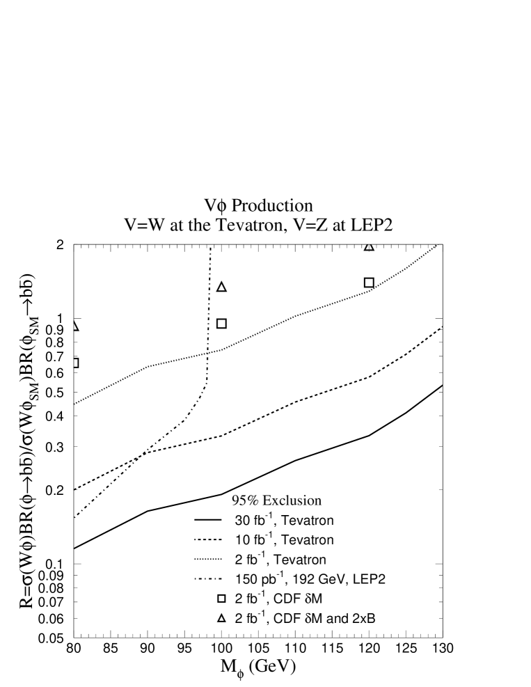
FIG. 1.: 95% C.L. bound on $R=\frac{\sigma(p\bar{p}\to W\phi)}{\sigma(p\bar{p}\to W\phi^{SM})}\frac{B(\phi\to b\bar{b})}{B(\phi^{SM}\to b\bar{b})}$ as a function of the Higgs boson mass for the Tevatron and LEP2.

FIG. 2.: Same as Fig. 1 except for $5\sigma$ discovery.

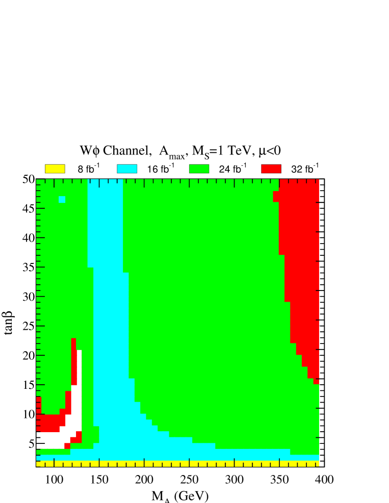
FIG. 3.: $5\sigma$ discovery contours for the $W\phi(\to b\bar{b})$ mode at the Tevatron in the MSSM for maximal mixing, $\mu<0$, and $M_{S}$=1 TeV. Different shadings correspond to different integrated luminosities.

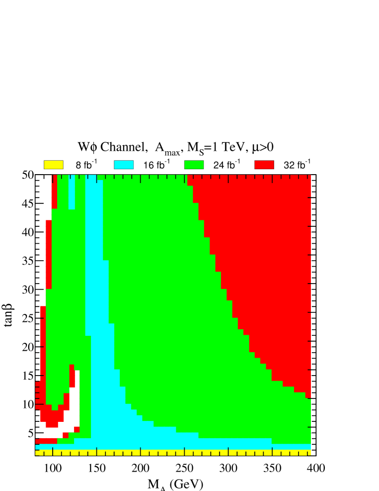
FIG. 4.: Same as Fig. 3 but with $\mu>0$.

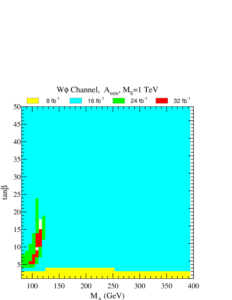
FIG. 5.: Same as Fig. 3 but for minimal mixing.

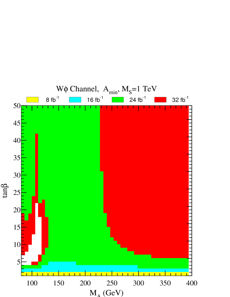
FIG. 6.: Same as Fig. 5 but using the present CDF mass resolution.

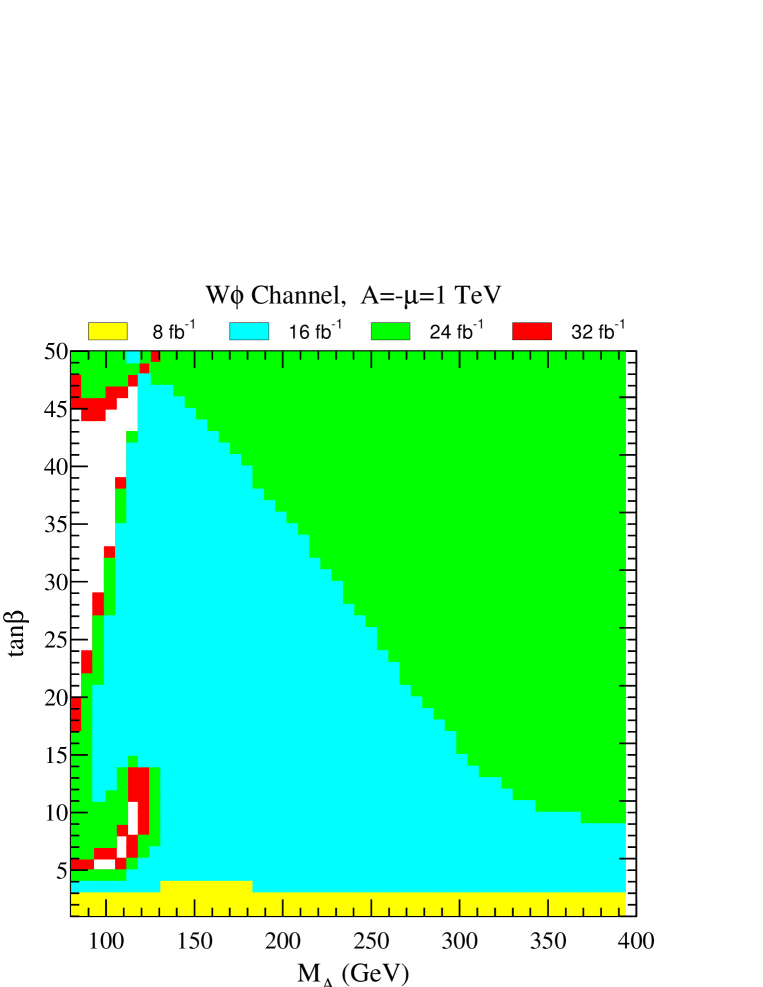
FIG. 7.: $5\sigma$ discovery contours for the $W\phi(\to b\bar{b})$ mode at the Tevatron for $A=-\mu=$ 1 TeV and $M_{S}=1$ TeV.

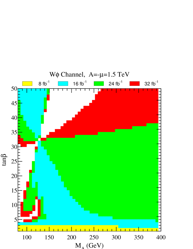
FIG. 8.: Same as Fig. 7 but for $A=-\mu=$ 1.5 TeV.

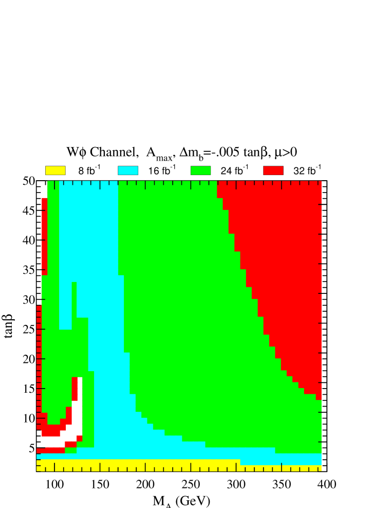
FIG. 9.: $5\sigma$ discovery contours for the $W\phi(\to b\bar{b})$ mode at the Tevatron for maximal mixing and $\mu>0$ after including large $\tan\beta$ corrections: $\Delta(m_{b})=-.005\tan\beta$. Different shadings correspond to different integrated luminosities.

FIG. 10.: Same as Fig. 9 but for $\Delta(m_{b})=-.01\tan\beta$.

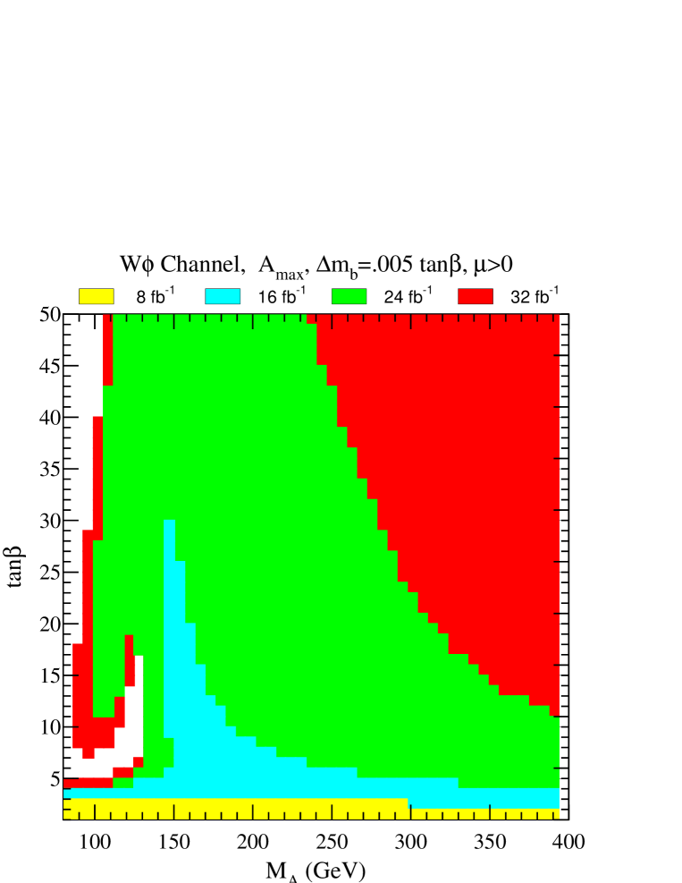
FIG. 11.: Same as Fig. 9 but for $\Delta(m_{b})=.005\tan\beta$.

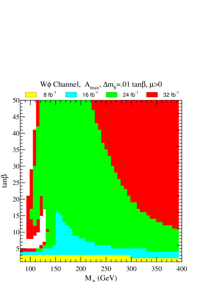
FIG. 12.: Same as Fig. 9 but for $\Delta(m_{b})=.01\tan\beta$.

FIG. 13.: Mass difference between the CP–odd Higgs boson and the CP–even Higgs boson (with properties similar to the CP–odd one) as a function of $\tan\beta$ for several MSSM parameter choices.

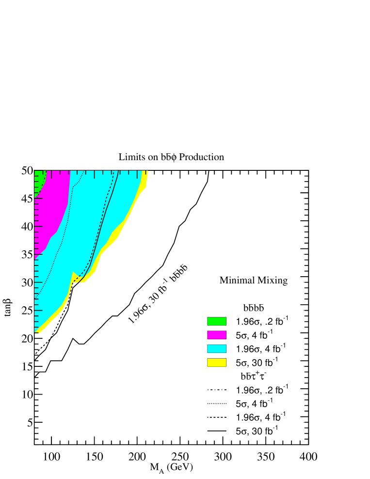
FIG. 14.: 95% C.L. exclusion and $5\sigma$ discovery contours for $b\bar{b}\phi$ production at the Tevatron in the MSSM for minimal mixing. The shaded areas correspond to different exclusion and discovery contours at different integrated luminosities for the $b\bar{b}b\bar{b}$ final state. The different lines show the same for the $b\bar{b}\tau^{+}\tau^{-}$ final state, except that the lower solid line shows the 95% C.L. exclusion contour for the $b\bar{b}b\bar{b}$ final state and 30 fb^-1.

FIG. 15.: $5\sigma$ discovery contours for the $b\bar{b}\phi(\to b\bar{b})$ mode and 30 fb^-1 with maximal mixing, $\mu>0$, and $\Delta(m_{b})=(0,\pm.005,\pm.01)\tan\beta$.