[
Pair Production in the Collapse of a Hopf Texture
Abstract
We consider the collapse of a global “Hopf” texture and examine the conjecture, disputed in the literature, that monopole-antimonopole pairs can be formed in the process. We show that such monopole-antimonopole pairs can indeed be nucleated in the course of texture collapse given appropriate initial conditions. The subsequent dynamics include the recombination and annihilation of the pair in a burst of outgoing scalar radiation.
]
I Introduction
An outstanding cosmological problem is explaining the homogeneity and isotropy of the universe on large scales while allowing for sufficient inhomogeneity and anisotropy on small scales to account for the existence of galaxies, stars, and, of course, us. Several mechanisms for this have been suggested. One of these is the inflationary scenario. An alternative which has also received considerable attention is the idea that the production of topological defects via phase transitions in the early universe provided the density fluctuations which eventually led to galaxy formation and the like.
In general, defects result because of a spontaneously broken symmetry. If one begins with a set of fields, , which possess a global symmetry and interact via a potential which breaks down to a subgroup , the vacuum manifold is described by the quotient space . Defects will arise in theories for which the vacuum manifold allows nontrivial homotopy groups characterized by an integer . The homotopy groups serve to differentiate mappings from the -dimensional sphere into the manifold [1]. For different values of , one gets different types of defects. Domain walls arise for , global strings for , monopoles for , and textures for .
At very early times, the universe is at a very high temperature so that, in general, the effective potential has a unique, symmetric vacuum state which does not allow defects. However, as the universe expands, it cools and passes through a symmetry breaking phase transition allowing for the possible formation of these defects. The vacuum manifold is no longer a single unique state, but instead a collection of degenerate vacuum states which comprise a nontrivial manifold. The presence of these defects can then serve as gravitational seeds for structure formation, and hence the importance of understanding their dynamics.
Here, we will be interested in a particular texture model and its dynamics. In accordance with Derrick’s theorem, scalar field configurations corresponding to a texture are unstable and will tend to shrink or collapse [1]. An interesting conjecture has recently been put forth on the collapse of various texture models. Sornborger et al [2] suggest that the nature of the various collapses can be categorized by whether the particular texture model allows more than one type of defect. In particular, models for which only is nontrivial (such as ) collapse in a similar (and, from their results, nearly indistinguishable) manner. On the other hand, models for which homotopy groups and are both nontrivial (such as ) should collapse in a qualitatively different manner, with the possible production of defects characterized by the other (non-) nontrivial homotopy group. These authors provide numerical evidence for their conjecture, having evolved several texture models from similar initial conditions and examined the collapse process/products.
The results in [2] would appear to be in agreement with interesting experimental evidence in nematic liquid crystals. Chuang et al [3] induce phase transitions in a nematic liquid crystal described by a broken symmetry and produce textures. These textures, they claim, decay via the production of a monopole-antimonopole pair. However, later numerical work by Rhie and Bennett [4] with this model suggests that such pair production did not occur. Later still, Luo [5] suggests that the reason for the absence of pair production in the numerical simulations of Rhie and Bennett is that the initial configuration of their simulations does not correspond to that seen in the laboratory experiments of Chuang. Instead, he presents different initial data which he claims should indeed nucleate monopoles.
In the following, we analyze the dynamics of collapsing Hopf textures, those textures occurring from the breaking of to . The results verify aspects of these earlier results and clarify the general picture. In the first section, we present the model, the evolution equations, and discuss the numerical approach. In subsequent sections, we consider the evolutions of a variety of initial data. These include a single monopole and a monopole-antimonopole pair which are evolved to demonstrate that the code can evolve these objects and to allow the identification of their presence or absence in later evolutions of texture collapse.
II The Equations and Numerical Approach
The model we consider is described by the Lagrangian
| (1) |
where the potential is
| (2) |
and is a set of three scalar fields. The scalar fields thus transform under the global symmetry group with the potential breaking this down to . The resulting vacuum manifold is for which the second and third homotopy groups are nontrivial. Thus this model allows both textures and global monopoles. The equations of motion are
| (3) |
A trivial rescaling invariance allows us to set , leaving the model with one free, dimensionless parameter .
Following [2] we split the total energy density into three parts: the kinetic, gradient and potential energy densities defined as
| (4) | |||||
| (5) | |||||
| (6) |
where an overdot denotes derivative with respect to time and represents the spatial gradient. The total energy density is
| (7) |
This model also has a conserved topological charge. The monopole current associated with the charge density is
| (8) |
where and are purely antisymmetric tensors of rank and respectively. The conserved monopole charge is
| (9) |
the integral of the charge density [6].
Given appropriate initial conditions, these equations are now straightforward to integrate in Cartesian coordinates. Some particular initial data that has been suggested for texture collapse is
| (13) |
where is the usual spherical radial coordinate and where the boundary conditions on the radial function are and . We discuss the evolution of this initial data as well as the evolution of another form of initial data for a texture in Sections V and VI.
It is worth noting that for the initial data in Eq.(13), the initial total energy density is axisymmetric. For the particular case in which , the initial energy is actually spherically symmetric. In addition, one may expect this axisymmetry to be maintained during the evolution. We attempt to take advantage of this observation and cast the equations and this initial data into a manifestly axisymmetric form. In cylindrical coordinates (), we define new quantities
| (14) | |||||
| (15) |
which, for the above initial data, can be seen to be manifestly axisymmetric. It is now a simple matter to get the equations of motion for . Using the equations of motion for from Eq.(3) we find the equations for to be
| (16) | |||||
| (17) | |||||
| (18) | |||||
| (19) |
with
| (20) |
Since the evolution will remain axisymmetric, we can discard the terms which have derivatives with respect to .
This simplification of the problem from 3D to 2D results in enormous gains from a computational perspective and allows us significant improvement in our potential resolution of dynamic features in the evolution. However, in our code development and tests, we found it very useful to also have a 3D code with which to compare our 2D results and results of earlier investigators.
For those reasons, we have implemented both a 3D code and a 2D axisymmetric code using a second order Crank-Nicholson finite difference scheme implemented with RNPL [7]. Out-going radiation conditions based on approximate spherical propagation as are imposed
| (21) |
for some function . This condition is very effective in limiting reflection from the boundaries. We have verified that these codes are fully convergent and that they are stable for many crossing times.
III Single Monopole
As stated in the introduction, we want to evolve a collapsing Hopf texture and examine the possible nucleation of monopole-antimonopole pairs. However, in order to understand the behavior of any nucleated monopoles modeled by these codes, we first examine the evolution of initial data explicitly containing a monopole. Using the standard hedgehog ansatz, we can represent a monopole of unit charge at the origin by
| (22) |
where
| (23) |
To find the static monopole , we substitute the ansatz (22) into Eq.(3) and set all time derivatives to zero
| (24) |
We then solve to find . However, instead of using the exactly static solution, , which is exact only in the continuum limit, we note that the static monopole is rather well approximated by
| (25) |
Using this as our initial data shows both the energy and monopole charge to be well conserved.
Because the monopole is a topological object, we expect that any initial data which has the same boundary conditions will also have unit topological charge. Hence, we can choose the function different than but still obeying Eq.(23) to set our initial data. This data will not be static but will still have a conserved monopole charge. As an example, we examine the evolution of initial data of the form
| (26) |
with and arbitrary constants.
These simulations have been done with time symmetric initial data. However, we have also implemented a boost of the monopole by giving it an initial velocity in some direction along an axis. The monopole is seen traversing the numerical domain. That we can evolve a monopole for many crossing times and also boost it while retaining its particle nature, provides further evidence that the global monopole is stable to radial perturbations as discussed in [8, 9, 10].
IV Monopole-Antimonopole Pair
Next, we would like to consider evolving a monopole-antimonopole pair with our codes. An anti-monopole is just a reflection of the monopole ansatz (22). Thus, it takes the form
| (27) |
Strictly speaking, there is not a superposition principle for monopoles and anti-monopoles. However, it is reasonable to assume that if the separation between the monopole and anti-monopole making up a pair is considerably larger than the core width of the respective particles, a pair configuration can be well approximated by matching a monopole solution to an anti-monopole solution. To achieve this, we translate the monopole up and the antimonopole down some distance to get the solution for a monopole-antimonopole pair located on the axis
| (28) |
where, in analogy with the previous section, we consider two forms for
| (29) |
and
| (30) |
At , the fields , though not differentiable, are continuous. This non-smoothness gets smoothed quickly by the numerical evolution and does not appear to affect the evolution of the pair significantly.
The total charge of this system during the evolution should be identically zero. Indeed, we confirm this numerically as the total charge remains essentially zero throughout the evolution. Though a necessary check for our code, this fact makes it a bit more difficult to follow the evolving charges individually. One quantity which we do track is the topological charge density. This, of course, should be peaked at the locations of the monopoles. However, we also found it useful to define and calculate a quantity which we call the “half-space charge.” It is simply the topological charge density integrated over positive only
| (31) |
We emphasize that this quantity has no topological meaning and is not necessarily conserved. However, as with our earlier argument for superposing the monopole-antimonopole pair, if we imagine the constituents of the pair to be well separated and individually well localized, the half-space charge should approximate the charge of the monopole (or anti-monopole).
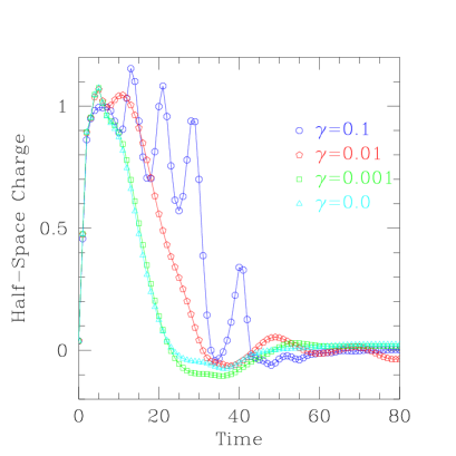
We then evolve the pair configuration for and show the resulting half-space charge in Fig. 1. Note that for early times, the average value of this quantity for large enough is roughly unity as we would expect for an isolated monopole. For smaller , the half-space charge becomes zero much more quickly. This behavior would appear consistent with the fact that decreasing has the effect of increasing the size of the respective monopoles. The increased size of the core makes it more difficult for us to associate the half-space charge with the true topological charge and results in more rapid pair annihilation.
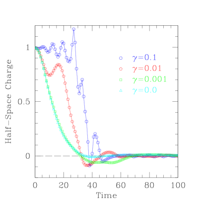
We have investigated the oscillations appearing in the half-space charge seen in Fig. 1. The oscillations converge with increasing resolution. Further, by moving the boundary farther from the monopole pair while keeping the same effective resolution, the oscillations remain the same. Both these results indicate that the oscillations are a real phenomenon and not a numerical artifact. Hence, the oscillations appear to be part of the dynamics. That this quantity oscillates is not inconsistent with charge conservation as this half-space charge is not a topological invariant. For it to be so, we would necessarily have to extend the integral out to infinity which we clearly cannot do while distinguishing the monopole from the pair. As further support that these oscillations are representative of the dynamics, oscillations of the total potential energy are observed to be correlated to the oscillations in the half-space charge.
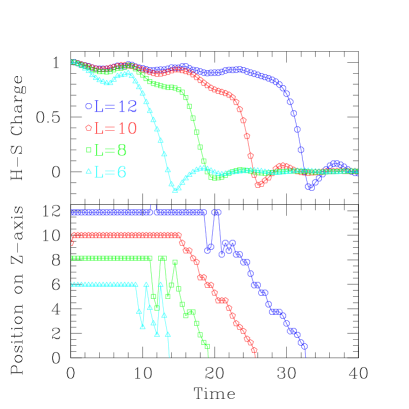
In Fig. 2, the results of varying the parameter in the pair configuration are shown. The graph of the half-space charge shows that the lifetime of the pair is clearly proportional to the initial separation. The bottom graph displays the position on the axis of the maximum charge density as a function of time. Because of our somewhat ad hoc matching procedure, the monopoles are not influenced by each other until a sufficient amount of time has passed for a signal to have propagated between them. At that point, the monopoles experience an attractive force, approach each other and annihilate.
V “Spherically Symmetric” Texture
With a good idea of what the signature of a monopole-antimonopole pair might be, we now evolve the initial data given in Eq.(13) with
| (32) |
Though the precise shape of this function does not appear to significantly affect the results, the function used here differs from that of [2] because the function shown there is not smooth.
As we stated in Section II, the total energy density is spherically symmetric only for . We are therefore being a bit careless to refer to this as spherically symmetric initial data. In addition, as shown in [2], symmetric configurations in the model we are considering are in fact unstable to nonspherical collapse. Nonetheless, we will continue to refer to the initial data described by Eq.(13) and Eq.(32) as “spherically symmetric” mainly to distinguish it from another set of initial data which we investigate that has toroidal symmetry.
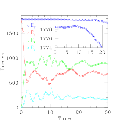
On evolving this data, we find that as the texture collapses, the energies evolve as described in [2]. The kinetic and gradient energies evolve towards equipartition while the potential energy remains a relatively small fraction of the total. Fig. 3 shows the energy versus time for the collapse of a typical “spherically symmetric” texture.
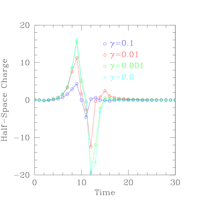
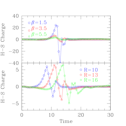
However, our results in both the 2D axisymmetric and the 3D codes do not bear out the claim that a monopole-antimonopole pair is formed [2]. As one indication, the half-space charge of the “spherically symmetric” texture as shown in Fig. 4 does not resemble that shown for the pair in Fig. 1. Fig. 4 suggests that there is a separation in the monopole charge density, but the duration of the resulting peaks in the charge density is independent of and the constant . Further, the half-space charge does not asymptote to as one might expect were a pair to form and move apart. This provides additional evidence that no monopoles are forming.
The half-space charge is also plotted for variations of and in Fig. 5. Again, the figure suggests that the “spherically symmetric” texture does not nucleate monopole pairs.
One measure, given in [2] and [4], for determining if a pair is present is that the potential energy density should be sharply peaked at the location of a monopole or antimonopole. We do see some peaking in the potential (and total) energy density for a brief period on the axis of symmetry, but the peaks do not persist. Indeed, these peaks quickly diminish in size and propagate off the grid with the remainder of the outgoing radiation (see further discussion in Section VII).
Thus we confirm earlier results of Rhie and Bennett [4] that pair production does not occur with this initial data in contradiction to that claimed in [2].
VI Toroidally Symmetric Texture
That the “spherically symmetric” texture does not collapse via the production of global monopoles does not exclude the possibility of pair production, merely our choice of initial data. Indeed, experiments with liquid crystals provide evidence that monopole pairs are in fact formed in Hopf texture collapse. For this reason, different initial data is suggested in [5] as possibly leading to pair creation. This initial data is toroidally symmetric. It is given by
| (33) | |||||
| (34) |
where, in terms of Cartesian coordinates , the toroidal coordinates are defined as
| (35) | |||||
| (36) | |||||
| (37) |
The parameter is the value of the so-called degenerate tori in this coordinate system. The function has boundary conditions (on the axis of symmetry and ) and (the degenerate torus). Thus a simple choice for is . Hence, we can write the initial data as
| (38) |
The evolutions of the toroidally symmetric texture generically display the creation of a monopole-antimonopole pair for all the values of we attempted. Fig. 6 shows the half-space charge for a typical run. These results are strikingly similar to those shown for the explicit pair evolved in Fig. 1. The charge begins at zero, quickly reaches a value approximately , and remains there until collapse. As is decreased, the behavior fundamentally changes in the same manner as that for the explicit pair. Hence, this charge separation appears intimately connected with the potential as would be expected for pair production. This connection is in contrast with the nearly -independent results of the “spherically symmetric” texture in Fig. 4.
Even more convincing evidence for the production of a monopole pair resides in actual movies made from the evolutions. Looking at either the potential energy density or total energy density, two peaks representing the monopoles occur along the axis of symmetry. The peaks leave the center of the grid, travel outward on the axis, and eventually switch direction and annihilate.
VII Discussion
The study of topological defects is important for studies of structure formation in cosmology, studies of superconductivity, liquid crystals, and superfluidity in condensed matter, and studies of regularity in topology.
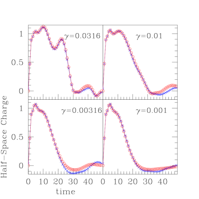
Here, we construct a code in 3D and in axisymmetry to model defect dynamics. Tests of the both codes show that they converge with increasing resolution and conserve energy. Further, the 3D code duplicates the results generated with the axisymmetric code as shown in Fig. 7.
Our code clarifies some of the conditions under which a Hopf texture nucleates a monopole-antimonopole pair. Specifically, our results confirm those of Rhie and Bennett [4] and Luo [5] that the “spherically symmetric” texture does not produce monopole pairs. This finding is in contradiction to the conclusion of [2]. However, our results are in agreement with their conjecture that models of texture collapse which allow more than one non-trivial homotopy group will evolve differently from those with just non-trivial . That toroidally symmetric initial data in this model leads to pair production agrees with their observation that these models can nucleate defects characterized by the non- homotopy group.
We speculate that the reason monopole production was claimed in [2] is that the collapse of a “spherically symmetric” texture does produce massive radiation in shells which are peaked along the axis. By examining an isosurface of the potential energy, apparent balls are seen radiating along the axis of symmetry. However, our evolutions suggest that observing isosurfaces can be deceiving. Indeed, by examining the charge density, no localization is observed.
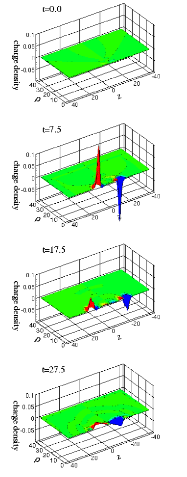
Consider, for example, Figs. 8 and 9. These show the charge densities for four snapshots in time for both the toroidally symmetric and “spherically symmetric” textures evolved using the 2D axisymmetric code. Examining the toroidally symmetric texture first, pair nucleation is quite dramatic between the first two frames. From an initially vanishing charge density, two localized, oppositely charged regions move outward from the origin. Between the last two frames, the monopoles change direction and move inward towards annihilation.
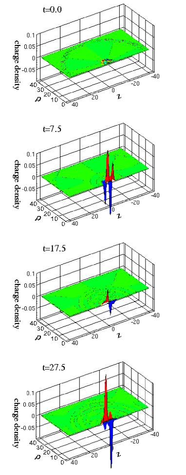
Contrast these dynamics with that shown in Fig. 9 for the “spherically symmetric” texture. Peaks in the charge density appear on the axis near the origin, but at no time are localized regions of non-vanishing charge density seen moving outward. Instead, the dynamics show only a region surrounding the origin in which the charge density oscillates. This is consistent with the form of the half-space charge in Figs. 3 and 4, which shows a steep rise and fall in this quantity.
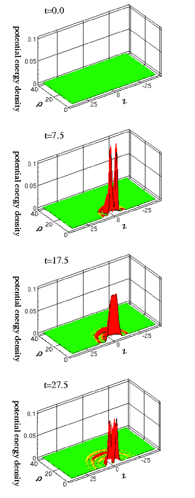
In addition, we show the potential energy density associated with these evolutions in Figs. 10 and 11. If monopoles exist in the space, then regions of non-zero charge density should be accompanied by trapped potential energy. For the toroidally symmetric texture, Fig. 10 demonstrates that the localized regions of non-zero charge density in Fig. 8 also contain localized potential energy. Note that these localized peaks in the potential energy maintain their distinct character until they recombine and annihilate. Hence, we conclude that this provides strong evidence that these localized regions represent monopoles.
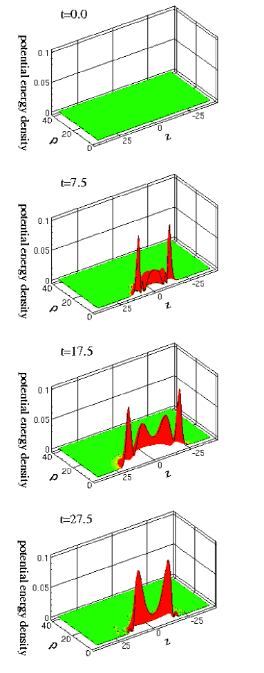
However, for the “spherically symmetric” texture shown in Fig. 11, the potential energy remains concentrated around the origin while shells of radiation move outward. Again, there is peaking in the potential energy density, however these concentrations do not maintain any distinct form. In particular, at times there are two peaks and at others there is only one in the strong field region near the origin. Outgoing radiation can be observed (this is seen more clearly in the evolutions) which is peaked along the axis, but these are not accompanied by a similar peaking in the charge density. Taken together, we therefore conclude from this evidence that no monopoles are nucleated with this initial data.
As we mentioned earlier, supplementary to these plots, we have produced movies of some of these evolutions. These evolutions can be viewed at http://godel.ph.utexas.edu/~ehirsch/hopf.html.
Both the axisymmetric and 3D codes are written in RNPL, an advanced numerical language developed at the Center [7]. Development of this language is ongoing, and we expect soon to have the ability to take advantage of automatic parallelization so that higher resolutions can be run. We also expect to adapt these codes to model other broken symmetries.
Acknowledgments
We would like to thank Matthew Choptuik and Andrew Sornborger for helpful discussions and correspondence. This work has been supported by NSF grants PHY9722068 and PHY9318152. These computations were done in part with support from a NPACI Metacenter Grant with time on the San Diego Supercomputer Center’s T90 machine.
REFERENCES
- [1] A. Vilenkin and E.P.S. Shellard, Cosmic Strings and Other Topological Defects, (Cambridge Press, Cambridge, 1994).
- [2] A. Sornborger, S.M. Carroll, and T. Pyne. Phys. Rev. D55, 6454-6456 (1997). hep-ph/9701351
- [3] I. Chuang, R. Durrer, N. Turok, B. Yurke, Science 251, 1336 (1991).
- [4] S.H. Rhie and D.P. Bennett, LANL preprint hep-ph/9206234 (1992).
- [5] X. Luo, Physics Letters B 287, 312-324 (1992).
- [6] R. Rajaraman, Solitons and Instantons, (North Holland Pub., New York, 1982).
- [7] R.L. Marsa and M.W. Choptuik, “The RNPL User’s Guide,” http://godel.ph.utexas.edu/Center/Rnpl_users_guide.html (1995).
- [8] D.P. Bennett and S.H. Rhie, Phys. Rev. Lett. 65, 1709-1712 (1990).
- [9] A.S. Goldhaber, Phys Rev. Lett. 63, 2158 (1989).
- [10] S.H. Rhie and D.P. Bennett, Phys Rev. Lett. 67, 1173 (1991).