Neutrino Propagation in Matter

Abstract

The enhancement of neutrino oscillations in matter is briefly reviewed. Exact and approximate solutions of the equations describing neutrino oscillations in matter are discussed. The role of stochasticity of the media that the neutrinos propagate through is elucidated.

1 Introduction

Particle and nuclear physicists devoted an increasingly intensive effort during the last few decades to searching for evidence of neutrino mass. Recent announcements by the Superkamiokande collaboration of the possible oscillation of atmospheric neutrinos [1] and very high statistics measurements of the solar neutrinos [2] brought us one step closer to understanding the nature of neutrino mass and mixings. Experiments imply that neutrino mass is small and the seesaw mechanism [3], to the development of which Dick Slansky contributed, is perhaps the simplest model which leads to a small neutrino mass.

If the neutrinos are massive and different flavors mix they will oscillate as they propagate in vacuum [4]. Dense matter can significantly amplify neutrino oscillations due to coherent forward scattering. This behavior is known as the Mikheyev-Smirnov-Wolfenstein (MSW) effect [5]. Matter effects may play an important role in the solar neutrino problem [6, 7, 8]; in transmission of solar [8] and atmospheric neutrinos [9, 10] through the Earth’s core; and shock re-heating [11] and r-process nucleosynthesis [12] in core-collapse supernovae. If the neutrinos have magnetic moments matter effects may also enhance spin-flavor precession of neutrinos [13].

The equations of motion for the neutrinos in the MSW problem can be solved by direct numerical integration, which must be repeated many times when a broad range of mixing parameters are considered. This often is not very convenient; consequently various approximations are widely used. Exact or approximate analytic results allow a greater understanding of the effects of parameter changes. The purpose of this article is to present a review of the solutions of the neutrino propagation equations in matter. Recent experimental developments and astrophysical implications of the neutrino mass and mixings are beyond the scope of this article. Very rapid developments make a medium such as the World Wide Web more suitable for the former and the latter was recently reviewed elsewhere [14]. Recent experimental developments can be accessed through the special home page at SPIRES [15] and theoretical results at the Institute for Advanced Study [16] and the University of Pennsylvania [17]. An assessment of the Superkamiokande solar neutrino data was recently given by Bahcall, Krastev, and Smirnov [6]. A number of recent reviews cover implications of recent results for neutrino properties [18].

2 Outline of the MSW Effect

The evolution of flavor eigenstates in matter is governed by the equation [5, 20]

$$i\hbar\frac{\partial}{\partial x}\left[\begin{array}[]{cc}\Psi_{e}(x)\\ \\ \Psi_{\mu}(x)\end{array}\right]=\left[\begin{array}[]{cc}\varphi(x)&\sqrt{\Lambda}\\ \\ \sqrt{\Lambda}&-\varphi(x)\end{array}\right]\left[\begin{array}[]{cc}\Psi_{e}(x)\\ \\ \Psi_{\mu}(x)\end{array}\right]\,,$$ (1)

where

$$\varphi(x)=\frac{1}{4E}\left(2\sqrt{2}\ G_{F}N_{e}(x)E-\delta m^{2}\cos{2\theta_{v}}\right)$$ (2)

for the mixing of two active neutrino flavors and

$$\varphi(x)=\frac{1}{4E}\left(2\sqrt{2}\ G_{F}\left[N_{e}(x)-\frac{N_{n}(x)}{2}\right]E-\delta m^{2}\cos{2\theta_{v}}\right)$$ (3)

for the active-sterile mixing. In these equations

$$\sqrt{\Lambda}=\frac{\delta m^{2}}{4E}\sin{2\theta_{v}},$$ (4)

$\delta m^{2}\equiv m_{2}^{2}-m_{1}^{2}$ is the vacuum mass-squared splitting, $\theta_{v}$ is the vacuum mixing angle, $G_{F}$ is the Fermi constant, and $N_{e}(x)$ and $N_{n}(x)$ are the number density of electrons and neutrons respectively in the medium.

In a number of cases adiabatic basis greatly simplifies the problem. By making the change of basis

$$\left[\begin{array}[]{cc}\Psi_{1}(x)\\ \\ \Psi_{2}(x)\end{array}\right]=\left[\begin{array}[]{cc}\cos{\theta(x)}&-\sin{\theta(x)}\\ \\ \sin{\theta(x)}&\cos{\theta(x)}\end{array}\right]\left[\begin{array}[]{cc}\Psi_{e}(x)\\ \\ \Psi_{\mu}(x)\end{array}\right]\,,$$ (5)

the flavor-basis Hamiltonian of Eq. (1) can be instantaneously diagonalized. The matter mixing angle in Eq. (5) is defined via

$$\sin{2\theta(x)}=\frac{\sqrt{\Lambda}}{\sqrt{\Lambda+\varphi^{2}(x)}}$$ (6)

and

$$\cos{2\theta(x)}=\frac{-\varphi(x)}{\sqrt{\Lambda+\varphi^{2}(x)}}\,.$$ (7)

In the adiabatic basis the evolution equation takes the form

$$i\hbar\frac{\partial}{\partial x}\left[\begin{array}[]{cc}\Psi_{1}(x)\\ \\ \Psi_{2}(x)\end{array}\right]=\left[\begin{array}[]{cc}-\sqrt{\Lambda+\varphi^{2}(x)}&-i\hbar\theta^{\prime}(x)\\ \\ i\hbar\theta^{\prime}(x)&\sqrt{\Lambda+\varphi^{2}(x)}\end{array}\right]\left[\begin{array}[]{cc}\Psi_{1}(x)\\ \\ \Psi_{2}(x)\end{array}\right]\,,$$ (8)

where prime denotes derivative with respect to $x$. Since the $2\times 2$ “Hamiltonian” in Eq. (8) is an element of the $SU(2)$ algebra, the resulting time-evolution operator is an element of the $SU(2)$ group. Hence it can be written in the form [19]

$$U=\left[\begin{array}[]{cc}\Psi_{1}(x)&-\Psi_{2}^{*}(x)\\ \\ \Psi_{2}(x)&\Psi_{1}^{*}(x)\end{array}\right]\,,$$ (9)

where $\Psi_{1}(x)$ and $\Psi_{2}(x)$ are solutions of Eq. (8) with the initial conditions $\Psi_{1}(x_{i})=1$ and $\Psi_{2}(x_{i})=0$. if the matter mixing angle, $\theta(x)$, is changing very slowly (i.e., adiabatically) its derivatives in Eq. (8) can be set to zero. In this approximation the “Hamiltonian” in the adiabatic basis is diagonal and the system remains in one of the matter eigenstates.

To calculate the electron neutrino survival probability Eq. (1) needs to be solved with the initial conditions $\Psi_{e}=1$ and $\Psi_{\mu}=0$. Using Eq. (9) the general solution satisfying these initial conditions can be written as

$$\Psi_{e}(x) = \cos{\theta(x)}[\cos{\theta_{i}}\Psi_{1}(x)-\sin{\theta_{i}}\Psi_{2}^{*}(x)]$$ (10)

$$+ \sin{\theta(x)}[\cos{\theta_{i}}\Psi_{2}(x)+\sin{\theta_{i}}\Psi_{1}^{*}(x)],$$

where $\theta_{i}$ is the initial matter angle. Once the neutrinos leave the dense matter (e.g. the Sun), the solutions of Eq. (8) are particularly simple. Inserting these into Eq. (10) we obtain the electron neutrino amplitude at a distance $L$ from the solar surface to be

$$\Psi_{e}(L) = \cos{\theta_{v}}[\cos{\theta_{i}}\Psi_{1,(S)}-\sin{\theta_{i}}\Psi_{2,(S)}^{*}]\exp{\left(i\frac{\delta m^{2}}{4E}L\right)}$$ (11)

$$+ \sin{\theta_{v}}[\cos{\theta_{i}}\Psi_{2,(S)}-\sin{\theta_{i}}\Psi_{1,(S)}^{*}]\exp{\left(-i\frac{\delta m^{2}}{4E}L\right)},$$

where $\Psi_{1,(S)}$ and $\Psi_{2,(S)}$ are the values of $\Psi_{1}(x)$ and $\Psi_{2}(x)$ on the solar surface. The electron neutrino survival probability averaged over the detector position, $L$, is then given by

$$P(\nu_{e}\rightarrow\nu_{e}) = \langle|\Psi_{e}(L)|^{2}\rangle_{L}=\frac{1}{2}+\frac{1}{2}\cos{2\theta_{v}}\cos{2\theta_{i}}\left(1-2|\Psi_{2,(S)}|^{2}\right)$$ (12)

$$- \frac{1}{2}\cos{2\theta_{v}}\sin{2\theta_{i}}\left(\Psi_{1,(S)}\Psi_{2,(S)}+\Psi_{1,(S)}^{*}\Psi_{2,(S)}^{*}\right)\,.$$

If the initial density is rather large, then $\cos{2\theta_{i}}\sim-1$ and $\sin{2\theta_{i}}\sim 0$ and the last term in Eq. (12) is very small. Different neutrinos arriving the detector carry different phases if they are produced over an extended source. Even if the initial matter density is not very large, averaging over the source position makes the last term very small as these phases average to zero. The completely averaged result for the electron neutrino survival probability is then given by [21]

$$P(\nu_{e}\rightarrow\nu_{e})=\frac{1}{2}+\frac{1}{2}\cos{2\theta_{v}}\langle\cos{2\theta_{i}}\rangle_{\rm source}\left(1-2P_{\rm hop}\right),$$ (13)

where the hopping probability is

$$P_{\rm hop}=|\Psi_{2,(S)}|^{2},$$ (14)

obtained by solving Eq. (8) with the initial conditions $\Psi_{1}(x_{i})=1$ and $\Psi_{2}(x_{i})=0$. Note that, since in the adiabatic limit $\Psi_{2,(S)}$ remains to be zero $P_{\rm hop}=0$.

3 Exact Solutions

Exact solutions for the neutrino propagation equations in matter exist for a limited class of density profiles that satisfy an integrability condition called shape invariance [22]. To illustrate this integrability condition we introduce the operators

$${\hat{A}}_{-} = i\hbar\frac{\partial}{\partial x}-\varphi(x)\,,$$

$${\hat{A}}_{+} = i\hbar\frac{\partial}{\partial x}+\varphi(x)\,.$$ (15)

Using Eq. (3) Eq. (1) takes the form

$${\hat{A}}_{-}\Psi_{e}(x) = \sqrt{\Lambda}\Psi_{\mu}(x)\,,$$

$${\hat{A}}_{+}\Psi_{\mu}(x) = \sqrt{\Lambda}\Psi_{e}(x)\,.$$ (16)

The shape invariance condition can be expressed in terms of the operators defined in Eq. (3) [23]

$${\hat{A}}_{-}(a_{1}){\hat{A}}_{+}(a_{1})={\hat{A}}_{+}(a_{2}){\hat{A}}_{-}(a_{2})+R(a_{1}).$$ (17)

We also introduce a similarity transformation which formally replaces $a_{1}$ by $a_{2}$:

$$\hat{T}(a_{1}){\cal O}(a_{1})\hat{T}^{-1}(a_{1})={\cal O}(a_{2}).$$ (18)

The MSW equations take a particularly simple form using the operators [24]

$$\hat{B}_{+} = \hat{A}_{+}(a_{1})\hat{T}(a_{1})$$

$$\hat{B}_{-} = \hat{T}^{-1}(a_{1})\hat{A}_{-}(a_{1})\,,$$ (19)

which satisfy the commutation relation:

$$[\hat{B}_{-},\hat{B}_{+}]=R(a_{0}),$$ (20)

where $a_{0}$ is defined using the identity

$$R(a_{n})=\hat{T}(a_{1})R(a_{n-1})\hat{T}^{-1}(a_{1}),$$ (21)

with $n=1$. Two additional commutation relations

$$[\hat{B}_{+}\hat{B}_{-},\hat{B}_{+}^{n}]=(R(a_{1})+R(a_{2})+\cdot\cdot+R(a_{n}))\hat{B}_{+}^{n},$$ (22)

and

$$[\hat{B}_{+}\hat{B}_{-},\hat{B}_{-}^{-n}]=(R(a_{1})+R(a_{2})+\cdot\cdot+R(a_{n}))\hat{B}_{-}^{-n}\,,$$ (23)

can easily be proven by induction.

Using the operators introduced in Eq. (3), Eq. (1) can be rewritten as

$${\hat{B}}_{+}{\hat{B}}_{-}\Psi_{e}(x)=\Lambda\Psi_{e}(x).$$ (24)

Eqs. (22) and (23) suggest that ${\hat{B}}_{+}$ and ${\hat{B}}_{-}$ can be used as ladder operators to solve Eq. (24). Introducing

$$\Psi_{-}^{(0)}\sim\exp{\left(-i\int\varphi(x;a_{1})dx\right)}.$$ (25)

one observes that

$${\hat{A}}_{-}(a_{1})\Psi_{-}^{(0)}=0={\hat{B}}_{-}\Psi_{-}^{(0)}.$$ (26)

If the function

$$f(n)=\sum_{k=1}^{n}R(a_{k})$$ (27)

can be analytically continued so that the condition

$$f(\mu)=\Lambda$$ (28)

is satisfied for a particular (in general, complex) value of $\mu$, then Eq. (22) implies that one solution of Eq. (24) is ${\hat{B}}_{+}^{\mu}\Psi_{-}^{(0)}$. Similarly the wavefunction

$$\Psi_{+}^{(0)}\sim\exp{\left(+i\int\varphi(x;a_{0})dx\right)}\,,$$ (29)

satisfies the equation

$${\hat{B}}_{+}\Psi_{+}^{(0)}=0.$$ (30)

Then a second solution of Eq. (24) is given by ${\hat{B}}_{-}^{-\mu-1}\Psi_{+}^{(0)}$. Hence for shape invariant electron densities the exact electron neutrino amplitude can be written as [24]

$$\Psi_{e}(x) = \beta{\hat{B}}_{+}^{\mu}\exp{\left(-i\int\varphi(x;a_{1})dx\right)}$$ (31)

$$+ \gamma{\hat{B}}_{-}^{-\mu-1}\exp{\left(+i\int\varphi(x;a_{0})dx\right)},$$

where $\beta$ and $\gamma$ are to be determined using the initial conditions $\Psi_{1}(x_{i})=1$ and $\Psi_{2}(x_{i})=0$.

For the linear density profile

$$N_{e}(x)=N_{0}-N_{0}^{\prime}(x-x_{R}),$$ (32)

where $N_{0}$ is the resonant density:

$$2\sqrt{2}\ G_{F}N_{0}E=\delta m^{2}\cos{2\theta_{v}},$$ (33)

using the technique described above we can easily write down the hopping probability

$$P_{\rm hop}=|\Psi_{2}(x_{f})|^{2}=\exp{(-\pi\Omega)}\,,$$ (34)

where

$$\Omega=\frac{\delta m^{2}}{4E}\frac{\sin^{2}{2\theta_{v}}}{\cos{2\theta_{v}}}\frac{N_{0}}{N_{0}^{\prime}}.$$ (35)

This is the standard Landau-Zener result [21, 25].

For the exponential density profile

$$N_{e}(x)=N_{0}e^{-\alpha(x-x_{R})},$$ (36)

where $N_{0}$ is the resonant density given in Eq. (33), the hopping probability is [26]

$$P_{\rm hop}=\frac{e^{-\pi\delta(1-\cos{2\theta_{v}})}-e^{-2\pi\delta}}{1-e^{-2\pi\delta}},$$ (37)

where we defined

$$\delta=\frac{\delta m^{2}}{2E\alpha}.$$ (38)

4 Supersymmetric Uniform Approximation

The coupled first-order equations for the flavor-basis wave functions can be decoupled to yield a second order equation for only the electron neutrino propagation

$$-\hbar^{2}\frac{\partial^{2}\Psi_{e}(x)}{\partial x^{2}}-\left[\Lambda+\varphi^{2}(x)+i\hbar\varphi^{\prime}(x)\right]\Psi_{e}(x)=0.$$ (39)

The large body of literature on the second-order differential equations of mathematical physics motivates using a semiclassical approximation for the solutions of Eq. (39). The standard semiclassical approximation gives the adiabatic evolution [27]. For a monotonically changing density profile supersymmetric uniform approximation yields [28]

$$P_{hop} = \exp(-\pi\Omega),$$

$$\Omega = \frac{i}{\pi}\frac{\delta m^{2}}{2E}\int^{r_{0}^{*}}_{r_{0}}dr\left[\zeta^{2}(r)-2\zeta(r)\cos{2\theta_{v}}+1\right]^{1/2}\,,$$ (40)

where ${r_{0}^{*}}$ and ${r_{0}}$ are the turning points (zeros) of the integrand. In this expression we introduced the scaled density

$$\zeta(r)=\frac{2\sqrt{2}G_{F}N_{e}(r)}{\delta m^{2}/E}\,,$$ (41)

where $N_{e}$ is the number density of electrons in the medium. By analytic continuation, this complex integral is primarily sensitive to densities near the resonance point. The validity of this approximate expression is illustrated in Figure 1.

Figure 1: The electron neutrino survival probability for the Sun [28]. The solid line is calculated using Eq.  (40). The dashed line is the exact (numerical) result. The dotted line is the linear Landau-Zener result. In the top figure, the lines are indistinguishable. An exponential density with parameters chosen to approximate the Sun was used [29].

As this figure illustrates the approximation breaks down in the extreme non-adiabatic limit (i.e., as $\delta m^{2}\rightarrow 0$). Hence it is referred to as the quasi-adiabatic approximation.

The near-exponential form of the density profile in the Sun [29] motivates an expansion of the electron number density scale height, $r_{s}$, in powers of density:

$$-r_{s}\equiv\frac{N_{e}(r)}{N_{e}^{\prime}(r)}=\sum_{n}b_{n}N_{e}^{n},$$ (42)

where prime denotes derivative with respect to $r$. In this expression a minus sign is introduced because we assumed that density profile decreases a $r$ increases. (For an exponential density profile, $N_{e}\sim e^{-\alpha x}$, only the $n=0$ term is present).

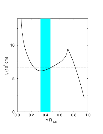
Figure 2: Electron number density scale height (cf. Eq. (42)) as a function of the radius for the Sun [29]. The dashed line is the exponential fit over the whole Sun. The shaded are indicates where the small angle MSW resonance takes place for neutrinos with energies $5<E<15$ MeV.

To help assess the appropriateness of such an expansion the density scale height for the Sun calculated using the Standard Solar Model density profile is plotted in Figure 2. One observes that there is a significant deviation from a simple exponential profile over the entire Sun. However the expansion of Eq. (42) needs to hold only in the MSW resonance region, indicated by the shaded area in the figure. Real-time counting detectors such as Superkamiokande and Sudbury Neutrino Observatory, which can get information about energy spectra, are sensitive to neutrinos with energies greater than about 5 MeV. For the small angle solution ($\sin 2\theta\sim 0.01$ and $\delta m^{2}=5\times 10^{-6}$ eV²), the resonance for a 5 MeV neutrino occurs at about 0.35 R_⊙ and for a 15 MeV neutrino at about 0.45 R_⊙ (the shaded area in the figure). In that region the density profile is approximately exponential and one expects that it should be sufficient to keep only a few terms in the expansion in Eq. (42) to represent the density profile of the Standard Solar Model.

Inserting the expansion of Eq. (42) into Eq. (40), and using an integral representation of the Legendre functions, one obtains [30]

$$\Omega = -\frac{\delta m^{2}}{2E}\left\{b_{0}(1-\cos{2\theta_{v}})\frac{}{}\right.$$ (43)

$$+ \sum^{\infty}_{n=1}\left(\frac{\delta m^{2}}{2\sqrt{2}G_{F}E}\right)^{n}\frac{b_{n}}{2n+1}\left.\left[P_{n-1}(\cos{2\theta_{v}})-P_{n+1}(\cos{2\theta_{v}})\right]\right\}\,,$$

where $P_{n}$ is the Legendre polynomial of order n. The $n=0$ term in Eq. (43) represents the contribution of the exponential density profile alone. Eq. (43) directly connects an expansion of the logarithm of the hopping probability in powers of $1/E$ to an expansion of the density scale height. That is, it provides a direct connection between $N_{e}(r)$ and $P_{\nu}(E_{\nu})$. Eq. (43) provides a quick and accurate alternative to numerical integration of the MSW equation for any monotonically-changing density profile for a wide range of mixing parameters.

Figure 3: (a) Spectrum distortion at SNO for the small-angle MSW solution ($\delta m^{2}\sim 5\times 10^{-6}$ eV² and $\sin 2\theta\sim 0.01$). The solid line is the exact numerical solution. The dashed, dot-dashed, and dotted lines result from values of $n$ up to 0, 1, and 2 in Eq. (43). The error bars on the exact numerical result correspond to two and five years of data collection. The dot-dot-dot-dashed line is the spectrum without MSW oscillations, normalized to the same total rate as with MSW oscillations. Note that on the scale of this figure the $n=1$ and $n=2$ lines are not distinguishable from the exact answer. (b) The relative error arising from the use of Eq. (43).

The accuracy of the expansion of Eq. (43) is illustrated in Figure 3 where the spectrum distortion for the small angle MSW solution is plotted. In this calculation we used the method of Ref. [31] and neglected backgrounds. The neutrino-deuterium charged-current cross-sections were calculated using the code of Bahcall and Lisi [32]. One observes that for the Sun, where the density profile is nearly exponential in the MSW resonance region, the first two terms in the expansion provide an excellent approximation to the neutrino survival probability.

5 Neutrino Propagation in Stochastic Media

In implementing the MSW solution to the solar neutrino problem one typically assumes that the electron density of the Sun is a monotonically decreasing function of the distance from the core and ignores potentially de-cohering effects [33]. To understand such effects one possibility is to study parametric changes in the density or the role of matter currents [34]. In this regard, Loreti and Balantekin [35] considered neutrino propagation in stochastic media. They studied the situation where the electron density in the medium has two components, one average component given by the Standard Solar Model or Supernova Model, etc. and one fluctuating component. Then the Hamiltonian in Eq. (1) takes the form

$$\hat{H}=\left({{-\delta m^{2}}\over 4E}\cos 2\theta+{1\over\sqrt{2}}G_{F}(N_{e}(r)+N^{r}_{e}(r))\right){\sigma_{z}}+\left({{\delta m^{2}}\over 4E}\sin 2\theta\right){\sigma_{x}}.$$ (44)

where one imposes for consistency

$$\langle N^{r}_{e}(r)\rangle=0,$$ (45)

and a two-body correlation function

$$\langle N^{r}_{e}(r)N^{r}_{e}(r^{\prime})\rangle={\beta}^{2}\ N_{e}(r)\ N_{e}(r^{\prime})\ \exp(-|r-r^{\prime}|/\tau_{c}).$$ (46)

In the calculations of the Wisconsin group the fluctuations are typically taken to be subject to colored noise, i.e. higher order correlations

$$f_{12\cdots}=\langle N^{r}_{e}(r_{1})N^{r}_{e}(r_{2})\cdots\rangle$$ (47)

are taken to be

$$f_{1234}=f_{12}f_{34}+f_{13}f_{24}+f_{14}f_{23},$$ (48)

and so on.

Mean survival probability for the electron neutrino in the Sun is shown in Figure 4 [36] where fluctuations are imposed on the average solar electron density given by the Bahcall-Pinsonneault model.

Figure 4: Mean electron neutrino survival probability in the sun with fluctuations. The average electron density is given by the Standard Solar Model of Bahcall and Pinsonneault [37] and $\sin^{2}2\theta=0.01$.

One notes that for very large fluctuations complete flavor de-polarization should be achieved, i.e. the neutrino survival probability is 0.5, the same as the vacuum oscillation probability for long distances. To illustrate this behavior the results from the physically unrealistic case of 50% fluctuations are shown. Also the effect of the fluctuations is largest when the neutrino propagation in their absence is adiabatic. This scenario was applied to the neutrino convection in a core-collapse supernova where the adiabaticity condition is satisfied [38]. Similar results were also obtained by other authors [39, 40, 41, 42]. It may be possible to test solar matter density fluctuations at the BOREXINO detector currently under construction [43]. Propagation of a neutrino with a magnetic moment in a random magnetic moment has also been investigated [35, 44]. Also if the magnetic field in a polarized medium has a domain structure with different strength and direction in different domains, the modification of the potential felt by the neutrinos due polarized electrons will have a random character [46]. Using the formalism sketched above, it is possible to calculate not only the mean survival probability, but also the variance, $\sigma$, of the fluctuations to get a feeling for the distribution of the survival probabilities [36] as illustrated in Figure 5.

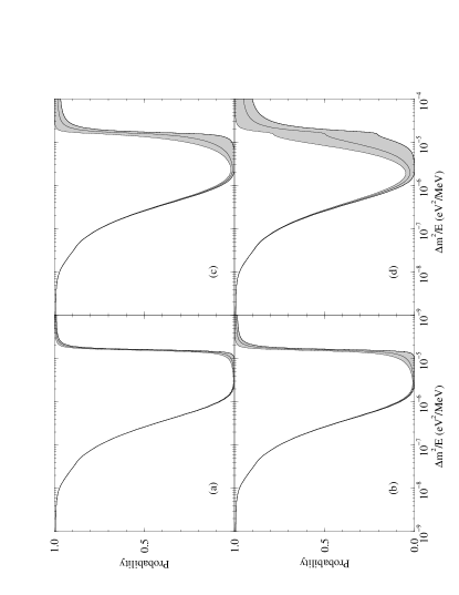
Figure 5: Mean electron neutrino survival probability plus minus $\sigma$ in the sun with fluctuations. The average electron density is given by the Standard Solar Model of Bahcall and Pinsonneault and $\sin^{2}2\theta=0.01$. Panels (a), (b), (c), and (d) correspond to an average fluctuation of 1%, 2%, 4%, and 8% respectively.

In these calculations the correlation length $\tau$ is taken to be very small, of the order of 10 km., to be consistent with the helioseismic observations of the sound speed [45]. In the opposite limit of very large correlation lengths are very interesting result is obtained [38], namely the averaged density matrix is given as an integral

$$\lim_{\tau_{c}\to\infty}\langle\hat{\rho}(r)\rangle={1\over{\sqrt{2\pi\beta^{2}}}}\int_{-\infty}^{\infty}dx\exp[{-x^{2}/(2\beta^{2})}]\hat{\rho}(r,x),$$ (49)

reminiscent of the channel-coupling problem in nuclear physics [47]. Even though this limit is not appropriate to the solar fluctuations it may be applicable to a number of other astrophysical situations.

References

- [1] Y. Fukuda, et al., (The Superkamiokande collaboration), hep-ex/9807003.
- [2] Y. Fukuda, et al., (The Superkamiokande collaboration), hep-ex/9805021.
- [3] M. Gell-Mann, P. Ramond, and R. Slansky, in Supergravity, P. van Nieuwenhuizen and D.Z. Freedman, Eds., North Holland, Amsterdam, 1979, p. 315; T. Yanagida, in Proceedings of the Workshop on the Unified Theory and Baryon Number in the Universe, O. Sawada and A. Sugamoto, Eds., (KEK Report 79-18, 1979), p.95.
- [4] B. Pontecorvo, Zh. Exp. Teor. Phys. 4 (1957) 549 [JEPT 6 (1958) 429].
-
[5]
S.P. Mikheyev and A. Yu. Smirnov,
Sov. J. Nucl. Phys. 42 (1985) 913; Sov. Phys. JETP 64 (1986) 4;
L. Wolfenstein, Phys. Rev. D 17 (1978) 2369; ibid. 20 (1979) 2634. - [6] J.N. Bahcall, P.I. Krastev, and A.Yu. Smirnov, hep-ph/9807216.
- [7] V. Barger, S. Pakvasa, T. J. Weiler, and K. Whisnant, hep-ph/9806328.
- [8] N. Hata and P. Langacker, Phys. Rev. D 56 (1997) 6107; M. Maris and S.T. Petcov, ibid. 7444.
- [9] Q.Y. Liu, S.P. Mikheyev, and A.Yu. Smirnov, hep-ph/9803415; E.K. Akhmedov, hep-ph/9805272.
- [10] S.T. Petcov, hep-ph/9805262.
- [11] G.M. Fuller, R.W. Mayle, B.S. Meyer, and J.R. Wilson, Astrophys. J. 389 (1992) 517; R.W. Mayle, in Supernovae, A.G. Petschek, Ed., (Springer-Verlag, New York, 1990).
- [12] Y.Z. Qian, G.M. Fuller, G.J. Mathews, R.W. Mayle, J.R. Wilson, and S.E. Woosley, Phys. Rev. Lett. 71 (1993) 1965; Y.Z. Qian and G.M. Fuller, Phys. Rev. D 52 (1995) 656; ibid. 51 (1995) 1479; H. Nunokawa, Y.Z. Qian, and G.M. Fuller, ibid. 55 (1997) 3265; W.C. Haxton, K. Langanke, Y.Z. Qian, and P. Vogel, Phys. Rev. Lett. 78 (1997) 2694; G.C. McLaughlin and G.M. Fuller, Astrophys. J. 464 (1996) L143.
- [13] C.-S. Lim and W.J. Marciano, Phys. Rev. D 37 (1988) 1368, E. Kh. Akhmedov, Phys. Lett. B 213 (1988); A.B. Balantekin, P.J. Hatchell, and F. Loreti, Phys. Rev. D 41 (1990) 3583.
- [14] A.B. Balantekin, in Proceedings of the VIII Jorge Andre Swieca Summer School on Nuclear Physics, C.A. Bertulani, M.E. Bracco, B.V. Carlson, M. Nielsen, Eds., (World Scientific, Singapore, 1998) (astro-ph/9706256); W.C. Haxton, Ann. Rev. Astron. Astrophys. 33 (1995) 459.
- [15] http://www.slac.stanford.edu/slac/announce/9806-japan-neutrino/ more.html
- [16] http://www.sns.ias.edu/jnb/.
- [17] http://dept.physics.upenn.edu/www/neutrino/solar.html.
- [18] See for example J.W.F. Valle, hep-ph/9712277; S. Pakvasa, hep-ph/9804426; W.C. Haxton, nucl-th/9712049.
- [19] R. Slansky, Phys. Rep. 79 (1981) 1.
- [20] H.A. Bethe, Phys. Rev. Lett. 56 (1986) 1305; S.P. Rosen and J.M. Gelb, Phys. Rev. D 34 (1986) 969; E.W. Kolb, M.S. Turner, and T.P. Walker, Phys. Lett. B 175 (1986) 478; V. Barger, K. Whisnant, S. Pakvasa, and R.J.N. Phillips, Phys. Rev. D 22 (1980) 2718.
- [21] W.C. Haxton, Phys. Rev. Lett. 57 (1986) 1271; S.J. Parke, ibid. 1275.
- [22] F. Cooper, A. Khare, and U. Sukhatme, Phys. Rep. 251 (1995) 267.
- [23] A.B. Balantekin, Phys. Rev. A 57 (1988) 4188.
- [24] A.B. Balantekin, Phys. Rev. D 58 (1988) 013001.
- [25] W.C. Haxton, Phys. Rev. D 35 (1987) 2352.
- [26] M. Bruggen, W.C. Haxton, and Y.-Z. Qian, Phys. Rev. D 51 (1995) 4028; see also S.T. Petcov, Phys. Lett. B 200 (1988) 373.
- [27] A.B. Balantekin, S.H. Fricke, and P.J. Hatchell, Phys. Rev. D 38 (1988) 935.
- [28] A.B. Balantekin and J.F. Beacom, Phys. Rev. D 54 (1996) 6323.
- [29] J.N. Bahcall, Neutrino Astrophysics, (Cambridge University Press, New York, 1989).
- [30] A.B. Balantekin, J.F. Beacom, and J.M. Fetter, Phys. Lett. B 427 (1988) 317.
- [31] J. N. Bahcall, P. I. Krastev, and E. Lisi, Phys. Rev. C 55 (1997) 494.
-
[32]
J.N. Bahcall and E. Lisi, Phys. Rev. D 54 (1996) 5417.
See also http://www.sns.ias.edu/
~jnb/SNdata/ deuteriumcross.html. - [33] R.F. Sawyer, Phys. Rev. D 42 (1990) 3908.
- [34] A. Halprin, Phys. Rev. D 34 (1986) 3462; A. Schafer and S.E. Koonin, Phys. Lett. B 185 (1987) 417; P. Krastev and A.Yu. Smirnov, Phys. Lett. B 226 (1989) 341, Mod. Phys. Lett. A 6 (1991) 1001; W. Haxton and W.M. Zhang, Phys. Rev. D 43 (1991) 2484.
- [35] F.N. Loreti and A.B. Balantekin, Phys. Rev. D 50 (1994) 4762.
- [36] A.B. Balantekin, J. M. Fetter, and F. N. Loreti, Phys. Rev. D 54 (1996) 3941.
- [37] J.N. Bahcall and M. H. Pinsonneault, Rev. Mod. Phys. 67 (1995) 781; J.N. Bahcall, S. Basu, and M. H. Pinsonneault, Phys. Lett. B 433 (1988) 1.
- [38] F.N. Loreti, Y.Z. Qian, G.M. Fuller, and A.B. Balantekin, Phys. Rev. D 52 (1995) 6664.
- [39] H. Nunokawa, A. Rossi, V.B. Semikoz, and J.W.F. Valle, Nucl. Phys. B 472 (1996) 495; J.W.F. Valle, Nucl. Phys. Proc. Suppl. 48 (1996) 137; A. Rossi, ibid. (1996) 384.
- [40] C.P. Burgess and D. Michaud, Ann. Phys. 256 (1997) 1; P. Bamert, C.P. Burgess, and D. Michaud, Nucl. Phys. B 513 (1998) 319.
- [41] E. Torrente-Lujan, hep-ph/9602398; hep-ph/9807361; hep-ph/9807371; hep-ph/9807426
- [42] K. Hirota, Phys. Rev. D 57 (1998) 3140.
- [43] H. Nunokawa, A. Rossi, V. Semikoz, and J.W.F. Valle, hep-ph/9712455.
- [44] S. Pastor, V.B. Semikoz, J.W.F. Valle, Phys. Lett. B 369 (1996) 301; S. Sahu, Phys. Rev. D 56 (1997) 4378; S. Sahu and V.M. Bannur, hep-ph/9806427.
- [45] J.N. Bahcall, M.H. Pinsonneault, S. Basu, and J. Christensen-Dalsgaard, Phys. Rev. Lett. 78 (1977) 17.
- [46] H. Nunokawa, V.B. Semikoz, A.Yu. Smirnov, and J.W.F. Valle, Nucl. Phys. B 501 (1997) 17.
- [47] A.B. Balantekin and N. Takigawa, Rev. Mod. Phys. 70 (1998) 441 (nucl-th/9708036).