We amplify previous discussions of the fine-tuning price to be paid by supersymmetric models in the light of LEP data, especially the lower bound on the Higgs boson mass, studying in particular its power of discrimination between different parameter regions and different theoretical assumptions. The analysis is performed using the full one-loop effective potential. The whole range of $\tan\beta$ is discussed, including large values. In the minimal supergravity model with universal gaugino and scalar masses, a small fine-tuning price is possible only for intermediate values of $\tan\beta$. However, the fine-tuning price in this region is significantly higher if we require $b-\tau$ Yukawa-coupling unification. On the other hand, price reductions are obtained if some theoretical relation between MSSM parameters is assumed, in particular between $\mu_{0}$, $M_{1/2}$ and $A_{0}$. Significant price reductions are obtained for large $\tan\beta$ if non-universal soft Higgs mass parameters are allowed. Nevertheless, in all these cases, the requirement of small fine tuning remains an important constraint on the superpartner spectrum. We also study input relations between MSSM parameters suggested in some interpretations of string theory: the price may depend significantly on these inputs, potentially providing guidance for building string models. However, in the available models the fine-tuning price may not be reduced significantly.

 

^a) SCIPP, University of California, Santa Cruz.
^b) Institute of Theoretical Physics, Warsaw University.
^c) Theory Division, CERN, CH 1211 Geneva 23, Switzerland.
^d) Institute für Theoretische Physik, Technische Universität München.

1 Introduction

To paraphrase Saint Augustine: ”May Nature reveal supersymmetry, but not yet.” This seems to be the message from LEP and other accelerator experiments, so far. There are tantalizing pieces of circumstantial evidence for supersymmetry at accessible energies, including the measured magnitudes of the gauge coupling strengths [1, 2] and the increasing indication that the Higgs boson may be relatively light [3, 4]. On the other hand, direct searches at LEP and elsewhere have so far come up empty-handed. In the case of LEP 2, the physics reach for many sparticles has almost been saturated, though the direct Higgs search still has excellent prospects.

In this context, it is natural to wonder whether the continuing absence of sparticles should disconcert advocates of the Minimal Supersymetric Extension of the Standard Model (MSSM). After all, the only theoretical motivation for the appearance of sparticles at accessible energies is in order to alleviate the fine tuning required to maintain the electroweak hierarchy [5], and sparticles become less effective in this task the heavier their masses. Since the problem of fine-tuning is a subjective one, it is not possible to provide a concise mathematical criterion for deciding whether enough is enough, already. Moreover, the fine tuning can be discussed only in concrete models for the soft supersymmetry breaking terms, and any conclusion refers to the particular model under consideration. The fine-tuning price may also depend on other, optional, theoretical assumptions.

The idea which we prefer to promote here is that, along with the overall increase in the fine-tuning price imposed by the data, any sensible objective measure of the amount of fine tuning becomes an interesting criterion for at least comparing the relative naturalness of various theoretical models and constraints, and – within a given framework – of different parameter regions.

We have recently shown that the latest LEP and other data which constrain the MSSM parameters significantly increased the requisite amount of fine tuning [6] compared with pre-LEP days. We used one particular measure [7, 8], namely $\Delta_{0}\equiv{\rm max}_{i}|a_{i}/M_{Z}^{2}(\partial M_{Z}^{2}/\partial a_{i})|$, where the $a_{i}$ are the input parameters of the MSSM (for other measures of fine tuning, see [9]). Our tree-level analysis clearly demonstrated several qualitative trends but, as an obvious improvement, one should use the best available theoretical tools to evaluate the fine tuning, including in particular the full one-loop effective potential of the MSSM  [10, 11]. Secondly, one should update the analysis with the most recent experimental information, in particular on the mass of the Higgs boson [12] and the new result for $BR(b\rightarrow s\gamma)$ [13].

With the above improvements in hand, in this paper we address anew the question of the necessary amount of fine tuning, with a particular view to the power of the fine-tuning price to discriminate between different parameter regions and different theoretical assumptions.

In Section 2 we recall our measure of fine tuning and discuss its various qualitative aspects in the supergravity-mediated scenario with universal gaugino and scalar masses (the minimal supergravity model). The particular role of the Higgs boson mass is elucidated. In Section 3 we present our full one-loop results for small and intermediate $\tan\beta$ in this model. In the first place, we confirm previous findings [10, 11] that including the full one-loop effective potential reduces the apparent amount of fine-tuning by about 30% at moderate $\tan\beta\sim 10$, and by much larger factors for both small and large $\tan\beta$. On the other hand, the latest experimental lower limit $M_{h}>90$ GeV for low $\tan\beta$ increases the price again, so that the fine-tuning price we find for low $\tan\beta$ is not very different from that in [6]. In the minimal supergravity model, for intermediate $\tan\beta$: $3<\tan\beta<15$, there still exist domains of the parameter space with moderate, ${\cal O}(10\%)$, fine-tuning. This result is obtained after including all available experimental constraints, including in particular $b\rightarrow s\gamma$, but with no constraint on the Yukawa sector.

In Section 4 we address the question of bottom-quark/tau Yukawa-coupling ($b-\tau$) unification [14] in the minimal model for small and intermediate $\tan\beta\mathrel{\hbox to0.0pt{\raise 2.15277pt\hbox{$<$}\hss}{\lower 2.15277pt\hbox{$\sim$}}}30$. We show that inclusion of one-loop corrections to the bottom-quark mass substantially enlarges the $\tan\beta$ region where $b-\tau$ unification is possible, albeit at the expense of a higher fine-tuning price. Furthermore, the interplay of the constraints from $b-\tau$ unification and $b\rightarrow s\gamma$ decay and the dependence on $\tan\beta$ is understood. The minimal model with both $b-\tau$ unification and the $b\rightarrow s\gamma$ constraint imposed has no regions of small fine tuning. However, it is stressed that $b\rightarrow s\gamma$ decay is an optional constraint, which can be relaxed if we admit some departure from the minimal model, e.g., some flavour structure in the up-squark mass matrices. Given such a generalization, regions with low fine tuning exist with or without $b-\tau$ unification.

In Section 5 we emphasize the dependence of the fine-tuning price on the choice of the set of independent soft mass parameters in a given model. In particular, we find that in the minimal supergravity model $\Delta_{0}$ may be significantly reduced if the parameters $\mu_{0}$ and $M_{1/2}$ or $A_{0}$ (depending on the value of $\tan\beta$) are considered as linearly dependent on each other. In some stringy models these parameters are indeed not independent, although the correlation may not be linear. As is briefly discussed in Section 6, we find that in one class of such models $\Delta_{0}$ may be minimized only in unphysical regions of the parameter space corresponding to small sparticle masses and/or the absence of electroweak symmetry breaking. Within the physical region of parameters in the models studied, the fine-tuning price may not be reduced significantly.

In Section 7 we discuss the case of large $\tan\beta>30$. Our main conclusion is that it remains attractive (with small fine-tuning) for non-universal Higgs boson mass parameters at the GUT scale. Section 8 contains our conclusions.

2 Measure of Fine Tuning and Tree-Level Discussion

We first specify more precisely the fine-tuning criterion we use. Following [7, 8], we consider the logarithmic sensitivities of $M_{Z}$ with respect to variations in input parameters $a_{i}$:

$$\Delta_{a_{i}}={a_{i}\over M_{Z}}{\partial M_{Z}\over\partial a_{i}}$$ (1)

Note that here we take derivatives of $M_{Z}$ and not, as in [6], of $M^{2}_{Z}$: hence our $\Delta_{a_{i}}$ are smaller by factors 2, other things being equal. We then define

$$\Delta_{0}\equiv{\rm max}|\Delta_{a_{i}}|$$ (2)

It is clear that the fine tuning can be discussed only in concrete models for the soft supersymmetry breaking terms, and with a specified scale for their generation. Calculation of the derivatives (1) requires minimization of the effective scalar potential written in terms of the $a_{i}$. In the first approximation one may use (as we did in our previous paper) the tree-level form of the potential, but it is known [10] and has been strongly re-emphasized recently [11] that reliable quantitative analysis requires use of the full one-loop effective potential. This is particularly important for low and large values of $\tan\beta$, where one-loop corrections to the tree-level potential are decisive for electroweak symmetry breaking. In this paper we follow the one-loop approach of [10].

It is, nevertheless, useful to discuss first certain qualitative features of our analysis starting with the tree-level potential:

$$V = m^{2}_{1}|H_{1}|^{2}+m_{2}^{2}|H_{2}|^{2}+B\mu(\epsilon H_{1}H_{2}+\epsilon\bar{H}_{1}\bar{H}_{2})$$ (3)

$$+ {1\over 8}(g^{2}+g^{\prime 2})(|H_{1}|^{2}-|H_{2}|^{2})^{2}+{g^{2}\over 2}|\bar{H}_{1}H_{2}|^{2}$$

The derivatives (1) then read

$$\Delta_{a_{i}}={2\over(t^{2}-1)^{2}}\sum_{j} \!\!\!\!\!\!\!\left\{\left(c_{B}^{i}c_{\mu}^{j}+c_{B}^{j}c_{\mu}^{i}\right)t(t^{2}+1)\left[{a_{i}a_{j}\over M_{Z}^{2}}+{a_{i}a_{j}\over M_{A}^{2}}\right]\right.$$ (4)

$$\left.\!\!\!-c_{1}^{ij}\left[(t^{2}+1){a_{i}a_{j}\over M_{Z}^{2}}+2t^{2}{a_{i}a_{j}\over M_{A}^{2}}\right]-c_{2}^{ij}~{}t^{2}\left[(t^{2}+1){a_{i}a_{j}\over M_{Z}^{2}}+2{a_{i}a_{j}\over M_{A}^{2}}\right]\right\}$$

where $t\equiv\tan\beta$ and the coefficients $c_{1,2}^{ij}$, $c_{B}^{i}$ and $c^{i}_{\mu}$ are defined by

$$m_{1,2}^{2}\left(M_{Z}^{2}\right)= \!\!\!\!\!\!\!\!\sum_{ij}c_{1,2}^{ij}a_{i}a_{j}\phantom{aaaa}c_{1,2}^{ij}=c_{1,2}^{ji}$$

$$B\left(M_{Z}^{2}\right)= \!\!\!\!\!\!\!\!\sum_{i}c_{B}^{i}a_{i}$$ (5)

$$\mu\left(M_{Z}^{2}\right)= \!\!\!\!\!\!\!\!\sum_{i}c_{\mu}^{i}a_{i}$$

The numerical values of the coefficients $c_{1,2}^{ij}$, $c_{B}^{i}$ and $c^{i}_{\mu}$ can be found by solving the renormalization-group (RG) equations [15, 16] for the running from some initial scale down to $M_{Z}$.

The most popular model, with some phenomenological backing, is the MSSM with universal gaugino and scalar masses $(M_{1/2},m_{0})$ at the input supergravity scale (or GUT scale), and a universal trilinear (bilinear) supersymmetry breaking parameter $A_{0}(B_{0})$. The model is then formulated in terms of these four parameters and the $\mu_{0}$ parameter. Important features of this model are strong correlations between soft terms: all scalar mass parameters are assumed to be equal. At present we do not have any convincing theory of soft terms and might equally well contemplate the possibility of other patterns for them, for instance of non-universal Higgs-boson masses and/or different sets of independent parameters. The amount of fine tuning depends on this choice, as discussed in Section 5. However, in this and the following Section we discuss the universal case with five independent parameters (the minimal supergravity model).

Several qualitative effects in the fine tuning of soft terms can be seen already from (4). In particular, we can discuss the typical magnitude of the derivatives taken with respect to the five parameters of the minimal supergravity model, with the scale of the generation of soft terms taken to be $M_{GUT}=2\times 10^{16}$ GeV. As an example, we consider the region of small $\tan\beta$, not far from the quasi-infrared fixed-point solution for the top-quark Yukawa coupling, in which the fine tuning is generically larger than for intermediate values of $\tan\beta$.

Using analytic solutions obtained in [15] for the coefficients $c_{1,2}^{ij}$, $c_{B}^{i}$ and $c^{i}_{\mu}$ as an expansion in the parameter

$$y\equiv Y_{t}/Y_{t}^{FP}$$ (6)

where $Y_{t}^{FP}$ is the fixed-point value for the top-quark Yukawa coupling $Y_{t}\equiv h^{2}_{t}/4\pi$, we can calculate the derivatives in eq. (4) explicitly. In the limit $y\rightarrow 1$ one gets:

$$\Delta_{\mu_{0}}=-{2\over(t^{2}-1)^{2}}\left[\left(t^{2}+1\right)^{2}{\mu^{2}\over M^{2}_{Z}}+t^{2}\left(4{\mu^{2}\over M^{2}_{A}}-1-{M_{A}^{2}\over M^{2}_{Z}}\right)\right]$$

$$\Delta_{M_{1/2}}\approx{t^{2}+1\over(t^{2}-1)^{2}}\left[\left(7t^{2}-1\right){M_{1/2}^{2}\over M^{2}_{Z}}+t\left({\mu M_{1/2}\over M^{2}_{Z}}+{\mu M_{1/2}\over M^{2}_{A}}\right)+{12t^{2}\over t^{2}+1}{M_{1/2}^{2}\over M^{2}_{A}}\right]$$

$$\Delta_{A_{0}}\approx-{t(t^{2}+1)\over(t^{2}-1)^{2}}\left[{\mu A_{0}\over M^{2}_{Z}}+{\mu A_{0}\over M^{2}_{A}}\right]$$ (7)

$$\Delta_{B_{0}}\approx{2t(t^{2}+1)\over(t^{2}-1)^{2}}\left({\mu B_{0}\over M^{2}_{Z}}+{\mu B_{0}\over M^{2}_{A}}\right)$$

$$\Delta_{m_{0}}\approx{1\over(t^{2}-1)^{2}}\left[(t^{2}+1)(t^{2}-2){m_{0}^{2}\over M^{2}_{Z}}-2t^{2}{m_{0}^{2}\over M^{2}_{A}}\right]$$

where we may consider the region $t\equiv\tan\beta\sim(1.5-2)$ to be consistent with our approximation $y\approx 1$ - qualitatively similar conclusions can be drawn for other values of $\tan\beta$, as long as the bottom quark Yukawa coupling is much smaller than $Y_{t}$. The parameter $\mu$ at the scale $M_{Z}$ is related to its initial value $\mu_{0}$ by the equation $\mu^{2}\approx 2\mu^{2}_{0}(1-y)^{1/2}$. We note that the largest derivatives are $\Delta_{\mu_{0}}$ and $\Delta_{M_{1/2}}$, and they are of opposite signs. For instance, for all parameters of order $M_{Z}$ (a situation already strongly excluded by the present experimental constraints) both are already greater than $\sim 10$ for $\tan\beta\sim 1.5$. They increase quadratically with the values of the parameters, and this is the reason why large fine tuning is found for low $\tan\beta$ within the experimentally-acceptable parameter range. The derivative $\Delta_{A_{0}}$ is also sizeable and may also play an important role, since large negative $A_{0}$ may be necessary [19] to satisfy the present Higgs-boson mass limit [12]. The derivative $\Delta_{m_{0}}$ is typically of little importance. For a given parameter set, the necessary fine tuning is determined by the maximal derivative (2). Any such set should be chosen consistent with the present experimental data and the constraints (correlations) imposed by proper electroweak symmetry breaking (see for instance [10, 20]).

Among the experimental constraints, a special role is played by the Higgs-boson mass limits. This effect can be isolated by imposing all the available experimental constraints except the lower limit on $M_{h}$. For a chosen value of $\tan\beta$, we get then some minimal value of $\Delta_{0}$, and the corresponding parameter set determines the mass of the Higgs boson

$$M^{2}_{h}=M^{2}_{Z}\cos^{2}2\beta+{3\alpha\over 4\pi s^{2}_{W}}{m^{4}_{t}\over M^{2}_{W}}\left[\log\left({M^{2}_{\tilde{t}_{2}}M^{2}_{\tilde{t}_{1}}\over m^{4}_{t}}\right)+\left({M^{2}_{\tilde{t}_{2}}-M^{2}_{\tilde{t}_{1}}\over 4m^{2}_{t}}\sin^{2}2\theta_{\tilde{t}}\right)^{2}\right.$$

$$\times\left.f(M^{2}_{\tilde{t}_{2}},M^{2}_{\tilde{t}_{1}})+{M^{2}_{\tilde{t}_{2}}-M^{2}_{\tilde{t}_{1}}\over 2m^{2}_{t}}\sin^{2}2\theta_{\tilde{t}}\log\left({M^{2}_{\tilde{t}_{2}}\over M^{2}_{\tilde{t}_{1}}}\right)\right]$$ (8)

where $f(x,y)\equiv 2-(x+y)/(x-y)\log(x/y)$. We display in (8) only the one-loop formula valid for $M_{A}\stackrel{{\scriptstyle>}}{{{}_{\sim}}}3M_{Z}$ [17], which is a good approximation to the two-loop RG-improved prescription [18] used in our numerical studies. Due to the logarithmic dependence of $M_{h}^{2}$ on the physical stop masses squared (which in turn are functions of the initial parameters) any departure from the “best” value of $M_{h}$, for fixed $\tan\beta$ and in the range allowed by the other constraints, transmits itself into an approximately exponential rise of $\Delta_{0}$. This happens for $M_{h}$ changing in both directions, towards values both smaller and larger than the “best” value. Thus, for a given $\tan\beta$, the Higgs boson mass is a crucial probe of fine tuning. We also recall [18] that the Higgs boson mass is maximal for large $|\tilde{A}_{t}|\equiv|A_{t}-\mu\cot\beta|$. Since $A_{t}$ is given by [15]

$$A_{t}\approx(1-y)A_{0}-{\cal O}(1-2)M_{1/2},$$ (9)

maximizing $M_{h}$ requires $\mu>0$ and large negative $A_{0}$. Hence the derivative $\Delta_{A_{0}}$ may be large in the low $\tan\beta$ region.

3 Results for Low and Intermediate $\tan\beta$

In this Section we discuss our full one-loop results in the minimal supergravity model with five independent parameters. It is appropriate to begin by re-emphasizing that the fine-tuning criterion is not a rigorous mathematical statement, but rather an intuitive physical preference and hence remains necessarily subjective. (For instance, as already mentioned, our present definition differs by a factor 2 from the one used in [6].) Nevertheless, for a chosen measure of fine-tuning, one can study in this model relative changes in the amount of fine tuning as a function of changing experimental limits and of the considered parameter range. Here we emphasize this use of the naturalness criterion.

We first recall the experimental constraints used in this analysis. The data we take into account include the precision electroweak data reported at the Jerusalem conference [4], which are dominated by those from LEP 1. We constrain MSSM parameters by requiring that $\Delta\chi^{2}<4$ in a global MSSM fit [21, 22, 23, 24]. The main effect of this constraint is a lower bound on the left-handed stop: $M_{\tilde{t}_{L}}\stackrel{{\scriptstyle>}}{{{}_{\sim}}}300-400$ GeV [23]. We also take into account the direct LEP 2 lower limits on the masses of sparticles [25] and Higgs bosons. For the latter, we base ourselves on the recent data reported in [12]. We use the limit $M_{h}>90$ GeV which, strictly speaking, is valid for the Standard Model Higgs boson. This is approximately valid also for the MSSM Higgs boson for small tan$\beta$, although there still exist small windows in the parameter space where the experimental limit is lower. We neglect this possibility in the present analysis.

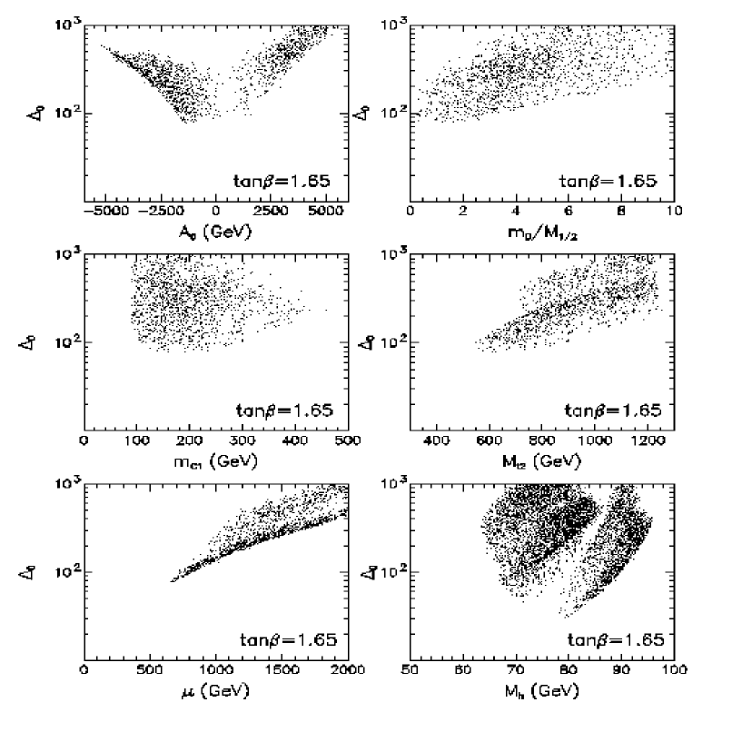
Figure 1: The price of fine tuning for $\tan\beta=1.65$, as a function of various variables in the minimal supergravity model. An upper limit of 1.2 TeV on the heavier stop mass is imposed in the scanning. All experimental constraints described in the text are included. In all plots, except for $\Delta_{0}$ versus $M_{h}$, the bound $M_{h}>90$ GeV is included. The mass of the lighter physical chargino and of the heavier physical stop are denoted by $m_{C1}$ and $M_{\tilde{t}_{2}}$, respectively.

The final accelerator contraint we use is the recently-measured value of the $b\rightarrow s\gamma$ branching ratio $2\times 10^{-4}<B(B\rightarrow X_{s}\gamma)<4.5\times 10^{-4}$ at the 95% C.L. [13]. The interpretation of this measurement in the MSSM is still subject to some uncertainty, because not all the ${\cal O}(\alpha_{s})$ corrections have yet been calculated. Resumming large QCD logaritms of the type $\log(M_{W}/m_{b})$ up to next-to-leading order (NLO) accuracy has recently been accomplished [26]. These calculations are identical in the SM and the MSSM. The initial numerical values of the Wilson coefficients at the scale $\mu\approx M_{W}$ are, however, different in the two models. In our analysis we have used for them two-loop results available for the standard $W^{\pm}t$ and $H^{\pm}t$ [27] contributions, and only the leading-order results for the chargino-stop contribution [28]. The uncertainty due to ${\cal O}(\alpha_{s}/\pi)$ corrections to them has been, however, included as in [29, 23]. Those references also contain extensive discussions of the role played by the $b\rightarrow s\gamma$ measurement in constraining the parameter space of the MSSM.

An important role may also be played by non-accelerator constraints, in particular the relic cosmological density of neutralinos $N^{0}$, if these are assumed to be the lightest supersymmetric particles, and if $R$ parity is absolutely conserved. Both of these assumptions may be disputed, and a complete investigation of astrophysical and cosmological constraints is beyond the scope of this analysis (for steps in this direction, see [30]).

One-loop corrections to the effective potential are taken into account as in [10], using the decoupling method of [31]. Numerical calculation of the derivatives $\Delta_{a_{i}}$ is also explained in [10]. Electroweak symmetry must, of course, be broken, and this requirement imposes strong constraints on the allowed parameter region. The main effect is that $\mu>{\rm max}(M_{1/2},~{}m_{0})$.

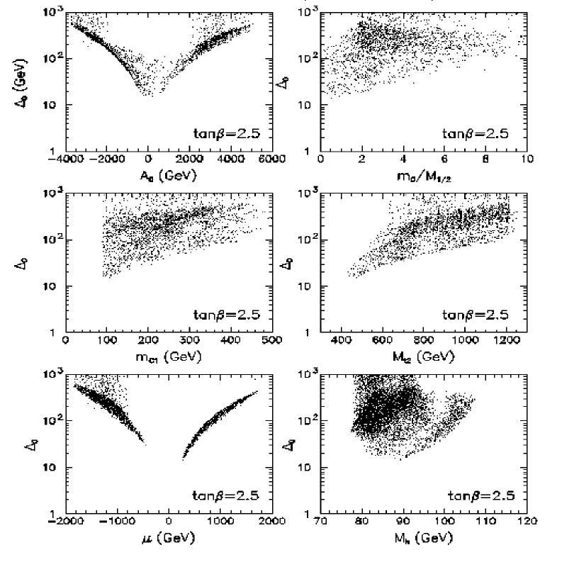
Figure 2: As in Fig. 1, but for $\tan\beta=2.5$.

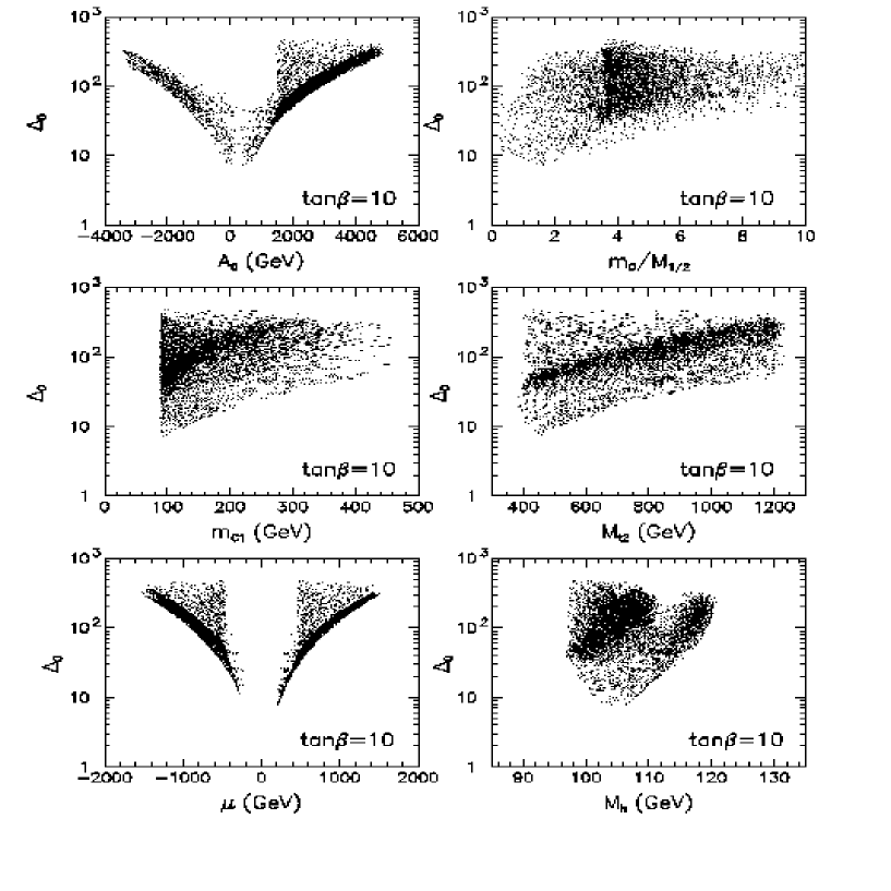
Figure 3: As in Fig. 1, but for $\tan\beta=10$.

In Figs. 1 to 3 we show $\Delta_{0}\equiv{\rm max}|\Delta_{a_{i}}|$ as a function of some mass parameters and some physical masses, for $\tan\beta=1.65$, 2.5 and 10. The results are in agreement with the qualitative discussion of Section 2 and with the results of [6], but the inclusion of one-loop corrections to the scalar potential sizeably decreases the fine-tuning price. For the same experimental constraints (in particular the same lower limit on $M_{h}$), the minimal value of $\Delta_{0}$ is for $\tan\beta=1.65$ a factor of $\sim 3-4$ smaller than in [6] (remember the factor 2 in the present definition of $\Delta_{0}$), in agreement with previous findings [10, 11]. For $\tan\beta\sim{\cal O}(10)$, one-loop corrections give much smaller effects, with typically a 30% reduction. In Figs. 1 to 3 we observe a very strong dependence of $\Delta_{0}$ on $M_{h}$, which has been explained in Section 2. In consequence, the new lower limit $M_{h}\stackrel{{\scriptstyle>}}{{{}_{\sim}}}90$ GeV [12] pushes, for $\tan\beta=1.65$, the minimal value of $\Delta_{0}$ into the range $\sim{\cal O}(100)$ ($\sim{\cal O}(200)$ with the definition of $\Delta_{0}$ used in [6]). We note the increase by a factor 3 in the minimal $\Delta_{0}$ with the change in the lower bound on $M_{h}$ from 80 to 90 GeV. The results in all three Figures are qualitatively similar except for the overall decrease in the fine-tuning price with increasing $\tan\beta$. One more difference is that the $\mu<0$ branch of solutions has disappeared at $\tan\beta=1.65$. For so small a value of $\tan\beta$, as explained earlier, negative $\mu$ is no longer compatible with the present bound $M_{h}>90$ GeV.

Figure 4: Fine-tuning measures as functions of $\tan\beta$. In panels (a),(c) and (e), lower limits on the Higgs boson mass of 90 GeV (solid), 100 GeV (long-dashed), 105 GeV (dashed) 110 GeV (dotted) and 115 GeV (dot-dashed) have been assumed. In panels (b), (d) and (f), $M_{h}$ has been fixed to 95 GeV (solid), 100 GeV (long-dashed), 105 GeV (dashed) 110 GeV (dotted) and 115 GeV (dot-dashed). Panels (a) and (b) correspond to independent $M_{1/2}$, $A_{0}$ and $\mu$ parameters. In panels (c), (d) and (e), (f), linear dependences $M_{1/2}=c_{M\mu}\mu_{0}$ and $A_{0}=c_{A\mu}\mu_{0}$, respectively, have been assumed.

The fine tuning decreases with increasing $\tan\beta$, with values of $\Delta_{0}$ marginally reaching $\Delta_{0}\approx 10$ for $3<\tan\beta<15$. This is shown in Fig. 4a, where we plot (solid line) the minimal $\Delta_{0}$ as a function of $\tan\beta$ for $M_{h}>90$ GeV. Also in Fig. 4a we show similar plots, but for hypothetical lower limits on the Higgs boson mass $M_{h}>100$, 105, 110 and 115 GeV. We notice that for $M_{h}>115$ GeV the fine-tuning is large for all values of $\tan\beta<30$. It is also interesting to observe that the bulk of the parameter range shown in Figs. 1 to 3 gives interestingly large fine tuning, even for intermediate values of $\tan\beta$. Finally, given the striking dependence of $\Delta_{0}$ on $M_{h}$, it is interesting to see its dependence on $\tan\beta$ under the assumption that we know the Higgs boson mass. In Fig. 4b this dependence is plotted for the hypothetical values $M_{h}=95$, 100, 105, 110 and 115 GeV. For values $M_{h}\leq 105$ GeV, $\Delta_{0}$ as a function of $\tan\beta$ has a clear minimum, which moves towards larger values of $\tan\beta$ with increasing $M_{h}$.

4 Bottom-Tau Yukawa Unification and $b\rightarrow s\gamma$ Decay

Up to now, we have been discussing fine tuning in the minimal supergravity model, without any constraints imposed on Yukawa couplings at the GUT scale. One important remark is that, in such a framework, the $b\rightarrow s\gamma$ decay, although constraining for the parameter space, does not have any impact on the necessary amount of fine tuning. The results for the minimal $\Delta_{0}$ presented in Figs. 1 to 3 and 4a does not depend at all on the inclusion of $b\rightarrow s\gamma$ decay among our experimental constraints for $\tan\beta\stackrel{{\scriptstyle<}}{{{}_{\sim}}}15$, and are negligibly modified for $\tan\beta$ up to 30. This is no longer true if we impose some constraints on the Yukawa sector, which is discussed in this Section and Section 7.

One interesting possibility is $b-\tau$ Yukawa-coupling unification at the GUT scale [14]. It is well known that exact $b-\tau$ Yukawa-coupling unification, at the level of two-loop renormalization group equations for the running from the GUT scale down to $M_{Z}$, supplemented by three-loop QCD running down to the scale $M_{b}$ of the pole mass and finite two-loop QCD corrections at this scale, is possible only for very small or very large values of $\tan\beta$. This is due to the fact that renormalization of the $b$-quark mass by strong interactions is too strong, and has to be partly compensated by a large $t$-quark Yukawa coupling. This result is shown in Fig. 5a. We compare there the running mass $m_{b}(M_{Z})$ obtained by the running down from $M_{GUT}$, where we take $Y_{b}=Y_{\tau}$, with the range of $m_{b}(M_{Z})$ obtained from the pole mass $M_{b}=(4.8\pm 0.2)$ GeV [34], taking into account the above-mentioned low-energy corrections. These translate the range of the pole mass: 4.6 $<M_{b}<$ 5.0 GeV into the following range of the running mass $m_{b}(M_{Z})$: $2.72<m_{b}(M_{Z})<3.16$ GeV. To remain conservative, we use $\alpha_{s}(M_{Z})=0.115(0.121)$ to obtain an upper (lower) limit on $m_{b}(M_{Z})$.

Figure 5: a) The running mass $m_{b}(M_{Z})$ obtained from strict $b-\tau$ Yukawa coupling unification at $M_{GUT}=2\times 10^{16}$ GeV for different values of $\alpha_{s}(M_{Z})$, before inclusion of one-loop supersymmetric corrections. b) The minimal departure from $Y_{b}=Y_{\tau}$ at $M_{GUT}$ measured by the ratio $Y_{b}/Y_{\tau}-1$, which is necessary for obtaining the correct $b$ mass in the minimal supergravity model with one-loop supersymmetric corrections included.

It is also well known [35, 36] that, at least for large values of $\tan\beta$, supersymmetric finite one-loop corrections (neglected in Fig. 5a) are very important. These corrections are usually not considered for intermediate values of $\tan\beta$ but, as we shall demonstrate, they are also very important there and make $b-\tau$ unification viable in much larger range of $\tan\beta$ than generally believed (see also [37]). However, one has then to pay a higher fine-tuning price!

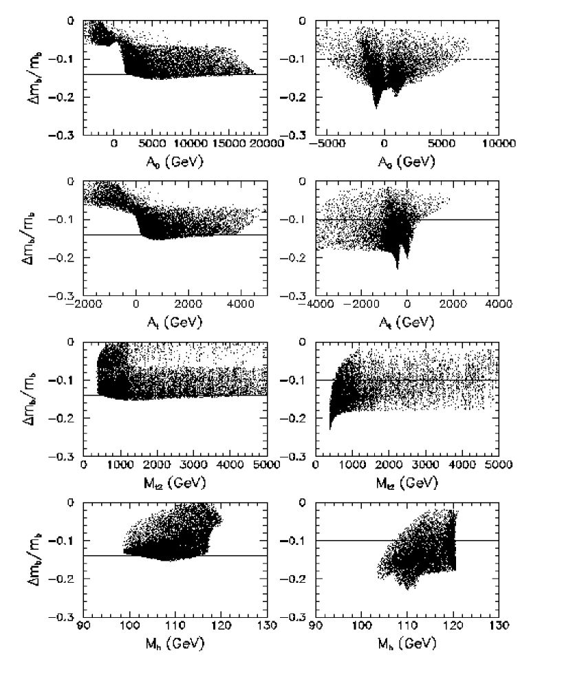
Figure 6: One-loop supersymmetric corrections to the $b$-quark mass as functions of various parameters for $\tan\beta=10$ (left panels) and 30 (right panels), assuming the minimal supergravity scenario and imposing all experimental cuts except for the $b\rightarrow s\gamma$ constraint. Acceptable values of $M_{b}$ are obtained for $\Delta m_{b}/m_{b}<-0.14$ for $\tan\beta=10$ and $\Delta m_{b}/m_{b}<-0.1$ for $\tan\beta=30$, corresponding to the regions below the solid horizontal lines.

One-loop diagrams with bottom squark-gluino and top squark-chargino loops make a contribution to the bottom-quark mass which is proportional to $\tan\beta$ [35, 36]. We recall that, to a good approximation, the one-loop correction to the bottom quark mass is given by the expression:

$${\Delta m_{b}\over m_{b}}\approx{\tan\beta\over 4\pi}\mu\left[{8\over 3}\alpha_{s}m_{\tilde{g}}I(m^{2}_{\tilde{g}},M^{2}_{\tilde{b}_{1}},M^{2}_{\tilde{b}_{2}})+Y_{t}A_{t}I(\mu^{2},M^{2}_{\tilde{t}_{1}},M^{2}_{\tilde{t}_{2}})\right]$$ (10)

where

$$I(a,b,c)=-{ab\log(a/b)+bc\log(b/c)+ca\log(c/a)\over(a-b)(b-c)(c-a)}$$

and the function $I(a,b,c)$ is always positive and approximately inversely proportional to its largest argument. This is the correction to the running $m_{b}(M_{Z})$. It is clear from Fig. 5a that for $b-\tau$ unification in the intermediate $\tan\beta$ region we need a negative correction of order (15-20)% for $3\mathrel{\hbox to0.0pt{\raise 2.15277pt\hbox{$<$}\hss}{\lower 2.15277pt\hbox{$\sim$}}}\tan\beta\mathrel{\hbox to0.0pt{\raise 2.15277pt\hbox{$<$}\hss}{\lower 2.15277pt\hbox{$\sim$}}}20$, and about a 10% correction for $\tan\beta=30$. According to (10), such corrections require $\mu<0$, and their dependence on some other parameters is shown in Fig. 6.

We notice that, as expected from (10), $b-\tau$ unification is easier for $\tan\beta=30$ than for $\tan\beta\approx 10$. In the latter case it requires $A_{t}\stackrel{{\scriptstyle>}}{{{}_{\sim}}}0$, in order to obtain an enhancement in (10) or at least to avoid any cancellation between the two terms in (10). This is a strong constraint on the parameter space. Since $A_{t}$ is given by (9),  $b-\tau$ unification requires large positive $A_{0}$ and not too large a $M_{\tilde{g}}$ (i.e., $M_{1/2}$). In addition, the low-energy value of $A_{t}$ is then always relatively small, and this explains the stronger upper bound on $M_{h}$ seen in Fig. 6 (for a similar conclusion, see [37]). We see in Fig. 5b that, for $\tan\beta\stackrel{{\scriptstyle<}}{{{}_{\sim}}}10$, the possibility of exact $b-\tau$ unification evaporates quite quickly, with a non-unification window for $2\stackrel{{\scriptstyle<}}{{{}_{\sim}}}\tan\beta\stackrel{{\scriptstyle<}}{{{}_{\sim}}}8-10$, depending on the value of $\alpha_{s}$. However, we also see that supersymmetric one-loop corrections are large enough to assure unification within 10% in almost the whole range of small and intermediate $\tan\beta$.

For $\tan\beta>10$, the qualitative picture changes gradually. The overall factor of $\tan\beta$, on the one hand, and the need for smaller corrections, on the other hand, lead to the situation where a partial cancellation of the two terms in (10) is necessary, or both corrections must be suppressed by sufficiently heavy squark masses. Therefore, as seen in Fig. 6 , $b-\tau$ unification for $\tan\beta=30$ typically requires a negative value of $A_{t}$, and is only marginally possible for positive $A_{t}$, for heavy enough squarks. A similar but more extreme situation occurs for very large $\tan\beta$ values, which will be discussed in Section 7. It is worth recalling already here that the second term in (10) is typically at most of order of (20-30)% of the first term [36], due to (9). Thus, cancellation of the two terms is limited, and for very large $\tan\beta$ the contribution of (10) must be anyway suppressed by requiring heavy squarks. This trend is visible in Fig. 7a already for $\tan\beta=30$. The Higgs-boson mass is not constrained by $b-\tau$ unification, since $A_{t}$ can be negative and large. Finally, we observe that, for any value of $\tan\beta$, the one-loop correction to $m_{b}(M_{Z})$ (10) remains approximately constant after simultaneous rescaling of $\mu$, $M_{1/2}$ and $m_{0}$. Since proper electroweak breaking correlates $\mu$ with $M_{1/2}$ and $m_{0}$, the loop correction to $m_{b}(M_{Z})$ is weakly dependent on sparticle masses.

Figure 7: a) Lower limits on the lighter (dotted lines) and heavier (solid lines) stop and on the $CP-$odd Higgs boson $A^{0}$ (dashed lines) in the minimal supergravity scenario with $b-\tau$ Yukawa coupling unification, as functions of $\tan\beta$. Upper (lower) lines refer to the case with the $b\rightarrow s\gamma$ constraint imposed (not imposed). b) The corresponding fine-tuning price with the $b\rightarrow s\gamma$ constraint imposed (solid line) and not imposed (dashed line).

Returning now to the fine-tuning price, we show in Fig. 7b the dependence of $\Delta_{0}$ on $\tan\beta$, with exact $b-\tau$ unification imposed as an additional constraint on the parameter space. This dependence is shown both without and with $b\rightarrow s\gamma$ decay included among the experimental constraints, and we first focus on the case with $b\rightarrow s\gamma$ excluded. A comparison with Fig. 3 (where $b-\tau$ unification was not imposed) shows a substantial increase in the fine-tuning price for $\tan\beta=10$. This follows from the large values of $A_{0}$ needed in this case for $b-\tau$ unification (see the strong dependence of $\Delta_{0}$ on $A_{0}$ in Fig. 3) and from the simultaneous ease in satisfying the $b\rightarrow s\gamma$ constraint for $\tan\beta\approx 10$ (as will be discussed shortly). On the other hand, for $\tan\beta=30$ it is easy to have $b-\tau$ unification. Hence, the price $\Delta_{0}$ to be paid without imposing the $b\rightarrow s\gamma$ constraint in Fig. 7b (dashed line) is essentially the same with or without $b-\tau$ unification (actually, it is slightly below the value seen in Fig. 4a for the case without $b-\tau$ unification but with the $b\rightarrow s\gamma$ constraint included).

We turn our attention now to a deeper understanding of the $b\rightarrow s\gamma$ constraint and its interplay with $b-\tau$ unification. The first point we would like to make is that $b\rightarrow s\gamma$ decay is a rigid constraint in the minimal supergravity model, but is only an optional one for the general low-energy effective MSSM. Its inclusion depends on the strong assumption that the stop-chargino-strange quark mixing angle is the same as the CKM element $V_{ts}$. This is the case only if squark mass matrices are diagonal in the super-KM basis, which is realized, for instance, in the minimal supergravity model. However, for the right-handed up-squark sector such an assumption is not imposed upon us by FCNC processes [38]. Indeed, aligning the squark flavour basis with that of the quarks, the up-type squark right-handed flavour off-diagonal mass squared matrix elements $(m^{2}_{\tilde{U}})^{13}_{RR}$ and $(m^{2}_{\tilde{U}})^{23}_{RR}$ are unconstrained by other FCNC processes. Therefore, in the limit that the other flavour off-diagonal matrix elements are zero, and for sufficiently small $(m^{2}_{\tilde{U}})^{23}_{RR}$, the couplings of charginos to stops and strange quark read

$${\cal L}_{int}\supset-\bar{s}\left(c_{R}^{ij}P_{R}+c_{L}^{ij}P_{L}\right)C^{-}_{j}{\tilde{t}}_{i}$$ (11)

with

$$c_{R}^{1j} \approx {e\over s_{W}}Z^{1j\star}_{+}V^{\star}_{ts}\sin\theta_{\tilde{t}}-Z^{2j\star}_{+}\left(h_{t}V^{\star}_{ts}+h_{c}{(m^{2}_{\tilde{U}})^{23}_{RR}\over M^{2}_{\tilde{c}_{R}}-M^{2}_{\tilde{t}_{1}}}\right)\cos\theta_{\tilde{t}}$$

$$c_{R}^{2j} \approx {e\over s_{W}}Z^{1j\star}_{+}V^{\star}_{ts}\cos\theta_{\tilde{t}}+Z^{2j\star}_{+}\left(h_{t}V^{\star}_{ts}+h_{c}{(m^{2}_{\tilde{U}})^{23}_{RR}\over M^{2}_{\tilde{c}_{R}}-M^{2}_{\tilde{t}_{2}}}\right)\sin\theta_{\tilde{t}}$$

$$c_{L}^{1j} = -h_{b}V^{\star}_{ts}Z^{2j}_{-}\sin\theta_{\tilde{t}}\phantom{aaaaaa}c_{L}^{2j}=-h_{b}V^{\star}_{ts}Z^{2j}_{-}\cos\theta_{\tilde{t}}$$ (12)

where $Z^{ij}_{\pm}$ are matrices diagonalizing the chargino mass matrix (defined in [32]), the $h_{t,b,c}$ are Yukawa couplings and the $\tilde{t}_{i}$ are stop mass eigenstates: $\tilde{t}_{R}=-\sin\theta_{\tilde{t}}\tilde{t}_{2}+\cos\theta_{\tilde{t}}\tilde{t}_{1}$. The factor $(\Delta^{R}m^{2})_{23}$ can be considered as a free parameter of the low-energy MSSM. Indeed, there exist GUT models [33] that predict the mixing factor in the vertex $\bar{s}\tilde{t}_{k}C_{i}^{-}$ to be considerably different from the CKM matrix element $V_{ts}$. We conclude that only a small departure from the minimal supergravity model is sufficient to relax the $b\rightarrow s\gamma$ constraint, and it is interesting to study separately its impact on the fine-tuning price.

In the minimal supergravity model the dominant contributions to $b\rightarrow s\gamma$ decay come from the chargino-stop and charged Higgs-boson/top-quark loops. For intermediate and large $\tan\beta$, one can estimate these using the formulae of [28] in the approximation of no mixing between the gaugino and higgsinos, i.e., for $M_{W}\ll max(M_{2},|\mu|)$. We get [39]

$${\cal A}_{W} \approx {\cal A}_{0}^{\gamma}{3\over 2}{m_{t}^{2}\over M_{W}^{2}}f^{(1)}\left({m_{t}^{2}\over M_{W}^{2}}\right)$$ (13)

$${\cal A}_{H^{+}} \approx {\cal A}_{0}^{\gamma}{1\over 2}{m_{t}^{2}\over M_{H^{+}}^{2}}f^{(2)}\left({m_{t}^{2}\over M_{H^{+}}^{2}}\right)$$ (14)

$${\cal A}_{C} \approx -{\cal A}_{0}^{\gamma}\left\{\left({M_{W}\over M_{2}}\right)^{2}\left[\cos^{2}\theta_{\tilde{t}}f^{(1)}\left({M_{\tilde{t}_{2}}^{2}\over M_{2}^{2}}\right)+\sin^{2}\theta_{\tilde{t}}f^{(1)}\left({M_{\tilde{t}_{1}}^{2}\over M_{2}^{2}}\right)\right]\right.$$

$$-\left({m_{t}\over 2\mu}\right)^{2}\left[\sin^{2}\theta_{\tilde{t}}f^{(1)}\left({M_{\tilde{t}_{2}}^{2}\over\mu^{2}}\right)+\cos^{2}\theta_{\tilde{t}}f^{(1)}\left({M_{\tilde{t}_{1}}^{2}\over\mu^{2}}\right)\right]$$

$$-\left.{\tan\beta\over 2}{m_{t}\over\mu}{m_{t}A_{t}\over M^{2}_{\tilde{t}_{2}}-M_{\tilde{t}_{1}}^{2}}\left[f^{(3)}\left({M_{\tilde{t}_{2}}^{2}\over\mu^{2}}\right)-f^{(3)}\left({M_{\tilde{t}_{1}}^{2}\over\mu^{2}}\right)\right]\right\}$$

where $\tilde{t}_{1}(\tilde{t}_{2})$ denotes the lighter (heavier) stop,

$$\cos^{2}\theta_{\tilde{t}}={1\over 2}\left(1+\sqrt{1-a^{2}}\right),\phantom{aaaaa}a\equiv{2m_{t}A_{t}\over M^{2}_{\tilde{t}_{2}}-M_{\tilde{t}_{1}}^{2}},\phantom{aaaaa}{\cal A}_{0}^{\gamma}\equiv G_{F}\sqrt{\alpha/(2\pi)^{3}}~{}V^{\star}_{ts}V_{tb}$$ (16)

and the functions $f^{(k)}(x)$ given in [28] are negative. The contribution ${\cal A}_{C}$ is effectively proportional to the stop mixing parameter $A_{t}$, and the sign of ${\cal A}_{C}$ relative to ${\cal A}_{W}$ and ${\cal A}_{H^{+}}$ is negative for $A_{t}\mu<0$.

We can discuss now the interplay of the $b-\tau$ unification and $b\rightarrow s\gamma$ constraints. The chargino-loop contribution (4) has to be small or positive, since the Standard Model contribution and the charged Higgs-boson exchange (both negative) leave little room for additional constructive contributions. Hence, one generically needs $A_{t}\mu<0$. Since $\mu<0$ for $b-\tau$ unification, both constraints together require $A_{t}>0$. This is in line with our earlier results for the proper correction to the $b$ mass for $\tan\beta\stackrel{{\scriptstyle<}}{{{}_{\sim}}}10$, but typically in conflict with such corrections for larger values of $\tan\beta$. In the latter case, both constraints can be satified only at the expense of heavy squarks (to suppress a positive $A_{t}$ correction to the $b$-quark mass or a negative $A_{t}$ correction to $b\rightarrow s\gamma$) and a heavy pseudoscalar $A^{0}$. Hence we have to pay a higher fine-tuning price, as seen in Figs. 7a,b.

5 Linear Relations between MSSM Parameters

The minimal supergravity model with universal soft mass parameters discussed so far is based on the assumption that scalar mass parameters are not independent of each other (and similarly for gaugino masses). This has obvious implications for the question of fine tuning, which can only be considered once the set of initial parameters is specified. In particular, one could relax the universality assumption and study the question of fine tuning for each sfermion flavour separately, with $\Delta_{\tilde{m}_{i}}$ being a measure of the fine tuning.. An increase (decrease) in the number of initial parameters is not directly correlated with increase or decrease of the necessary fine tuning. For instance, suppose the parameters $a_{i}$ and $a_{j}$ with derivatives $\Delta_{a_{i}}$ and $\Delta_{a_{j}}$ are assumed to be not independent but linearly related: $a_{i}=c_{ij}a_{j}$. In this new scenario, the fine tuning is measured by $\Delta_{a_{i}a_{j}}=\Delta_{a_{i}}+\Delta_{a_{j}}$. The relative magnitudes of $\Delta_{a_{i}a_{j}}$, $\Delta_{a_{i}}$ and $\Delta_{a_{j}}$ depend on the relative signs of $\Delta_{a_{i}}$ and $\Delta_{a_{j}}$, and vary from one region of parameters to another. However, as observed in [6] and indicated in Section 2, the scalar sector has little impact on the overall fine tuning, since the derivatives $\Delta_{\tilde{m}_{i}}$ are generically smaller than the other derivatives. Therefore, scenarios with correlated or uncorrelated scalar masses have similar fine tuning.

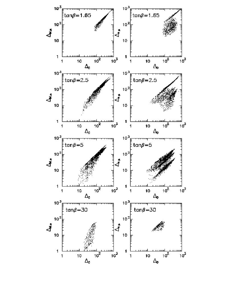
Figure 8: Fine-tuning for correlated GUT-scale parameters ($M_{1/2}=c_{M\mu}\mu_{0}$ in the left panels and $A_{0}=c_{A\mu}\mu_{0}$ in the right ones) versus fine tuning for uncorrelated GUT-scale parameters for several values of $\tan\beta$. Universal soft scalar masses are assumed at the GUT scale.

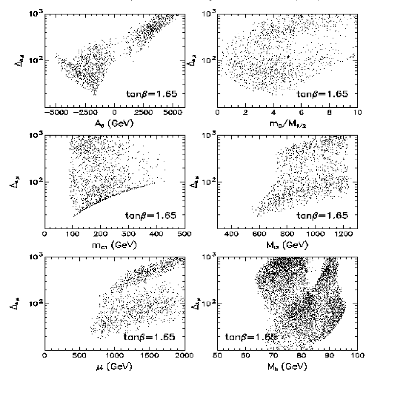
Figure 9: As in Fig. 1, but assuming the linear correlation $A_{0}=c_{A\mu}\mu_{0}$ at the GUT scale.

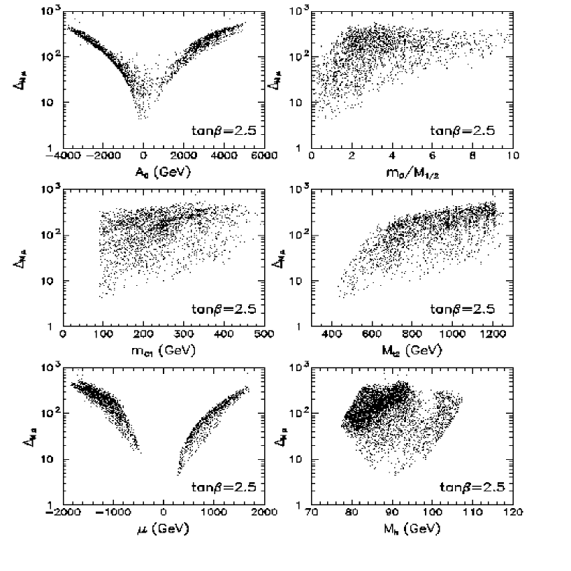
Figure 10: As in Fig. 2, but assuming the linear correlation $M_{1/2}=c_{M\mu}\mu_{0}$ at the GUT scale.

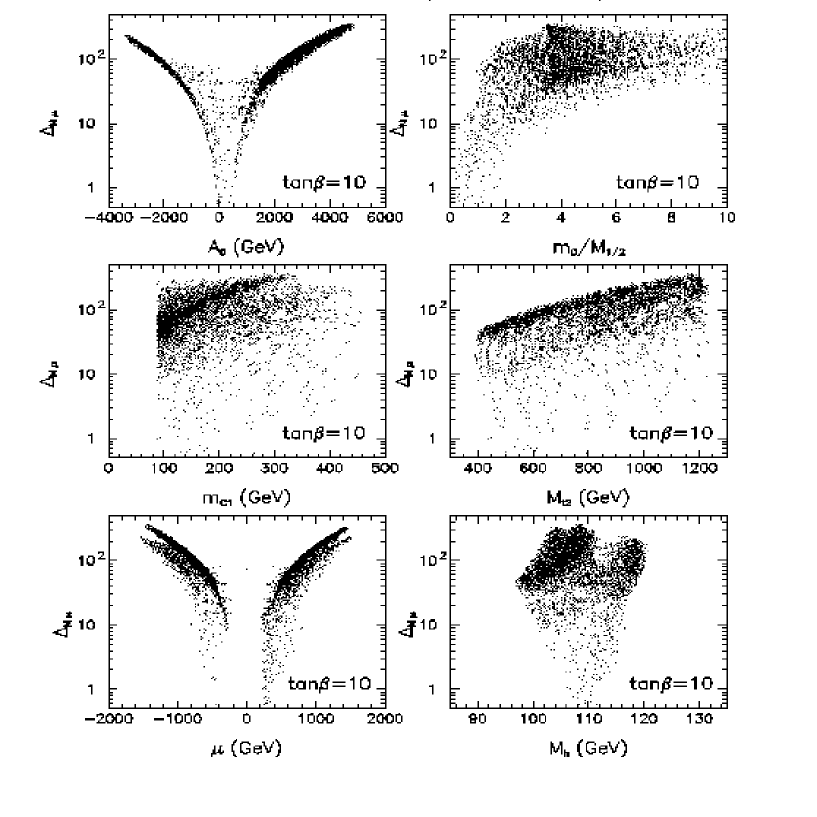
Figure 11: As in Fig. 3, but assuming the linear correlation $M_{1/2}=c_{M\mu}\mu_{0}$ at the GUT scale.

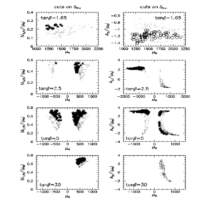
Figure 12: Correlations between the GUT scale parameters for several values of $\tan\beta$, assuming the following cuts on fine tuning. For $\tan\beta=1.65$: in the left panel, parameter sets with $\Delta_{M\mu}<50$ are indicated by stars, and sets with $\Delta_{M\mu}<100$ by points, in the right panel, sets with $\Delta_{A\mu}<20$ are indicated by by stars, $\Delta_{A\mu}<30$ by circles and $\Delta_{A\mu}<50$ by points. For $\tan\beta=2.5$ and 5: sets with $\Delta_{M\mu},\Delta_{A\mu}<10$ are indicated by stars and $\Delta_{M\mu},\Delta_{A\mu}<30$ by points. For $\tan\beta=30$: in the left panel, sets with $\Delta_{M\mu}<3$ are indicated by stars and $\Delta_{M\mu}<10$ by points, and in the right panel sets with $\Delta_{A\mu}<30$ are indicated by points.

The discussion in Section 2 shows that most often the largest derivatives are $\Delta_{\mu_{0}}$, $\Delta_{M_{1/2}}$ and $\Delta_{A_{0}}$ and, moreover, in the phenomenologically relevant parameter space they are of opposite signs. Let us take as an example again small $\tan\beta$. We see in (7) that $\Delta_{\mu_{0}}<0$, whereas $\Delta_{M_{1/2}}>0$ for $\mu>0$, which is necessary to maximize $M_{h}$. Also, sign$(\Delta_{A_{0}})=-$sign$(\mu A_{0})$, so that for $\mu>0$, sign$(\Delta_{\mu_{0}}\Delta_{A_{0}})$=sign$(A_{0})$ and for negative $A_{0}$ the derivatives $\Delta_{\mu_{0}}$ and $\Delta_{A_{0}}$ are of opposite signs. Since negative $A_{0}$ is necessary for maximizing $M_{h}$, one expects that, by assuming there is some theoretical reason why some of these parameters are not independent, one may significantly reduce the fine-tuning price. It is easy to study the simplest case of linear relations between these parameters. Linear relations are also enough to obtain substantial reductions in the fine tuning, as we find in our full one-loop numerical calculations.

Figure 13: Upper limit on the lighter stop (a), stau (b), chargino (c) and neutralino (d) as functions of $\tan\beta$ for universal soft scalar masses at the GUT scale requiring the fine-tuning measures $\Delta_{0}$ (solid), $\Delta_{M\mu}$ (dashed) and $\Delta_{A\mu}$ (dotted) smaller than 10.

We obtain the biggest reduction in the fine-tuning price by treating $M_{1/2}$ and $\mu_{0}$, or $A_{0}$ and $\mu_{0}$, as linearly related to each other, and the best choice depends on the value of $\tan\beta$. This is shown in Fig. 8, where we plot $\Delta_{0}$ versus $\Delta_{M_{1/2}\mu_{0}}$ and $\Delta_{A_{0}\mu_{0}}$ for several values of $\tan\beta$. For low $\tan\beta$ (close to the infrared quasi-fixed point) the best effect is obtained for the $A_{0}-\mu_{0}$ correlation, with the minimal fine tuning decreasing by a factor $\sim 3.5$. In Figs. 4c and 4e we plot minimal values of $\Delta_{M_{1/2}\mu}$ and $\Delta_{A_{0}\mu}$ as functions of $\tan\beta$ for several assumed limits on $M_{h}$: $M_{h}>90$, 100, 105, 110 and 115 GeV, and in Figs. 4d and 4f we show similar plots but for $M_{h}=95$, 100, 105, 110 and 115 GeV. The strong price reductions are evident. We see that $\Delta\sim{\cal O}(1)$ is compatible with a large range of $\tan\beta$ values and Higgs boson masses. In Figs. 9, 10 and 11, we plot $\Delta_{M_{1/2}\mu_{0}}$ and $\Delta_{A_{0}\mu_{0}}$ as functions of various mass parameters or physical masses, for several values of $\tan\beta$. The overall pattern remains similar to the $\Delta_{0}$ case, but with an order of magnitude or more rescaling in the absolute values of the $\Delta$’s. Nevertheless, putting some upper bound on the acceptable fine tuning remains a strong constraint on the superparticle spectrum. This is more clearly seen in Fig. 13, where we plot the upper bounds on several physical masses as a function of $\tan\beta$, as obtained by requiring $\Delta_{0}<10$. In this plot we compare the bounds obtained for $M_{1/2}-\mu_{0}$ and $A_{0}-\mu_{0}$ correlations with the bounds for the uncorrelated case ($\Delta_{0}<10$). As is seen clearly in Fig. 13, the upper bounds are considerably relaxed if correlations are imposed, suggesting that it is premature to use the fine-tuning price to derive convincingly any upper mass limits, in the absence of deeper theoretical understanding.

6 String-Inspired Models

So far, we have discussed linear dependences among soft supersymmetry-breaking terms in a model-independent way. We now take a more theoretical viewpoint, according to which the soft supersymmetry breaking parameters are predicted by some physics at the GUT or string scale. It is likely that they will emerge from the high-scale theory described in terms of more fundamental parameters. It is also plausible that the number of these parameters, at least of the relevant ones, is smaller than the number of soft terms. The latter will then not be independent. Such scenarios indeed emerge in various toy supergravity/string models for soft terms. The fine-tuning criterion would then require some revision: even if the number of new parameters is not smaller than the number of soft terms discussed earlier, a reparametrization may introduce more “natural” fundamental parameters. Generically, in supergravity models, one can write the soft terms as

$$a_{i}=m_{3/2}f_{i}\left(p_{\alpha}\right)$$ (17)

where $a_{i}$ is one of the soft supersymmetry-breaking terms ($M_{1/2}$, $m_{0}$, $A_{0}$, $B_{0}$), or $\mu_{0}$, and the gravitino mass $m_{3/2}$ sets the overall mass scale. The functions $f_{i}(p_{\alpha})$ are functions of dimensionless parameters $p_{\alpha}$ which can be regarded as, e.g., angles determining the goldstino direction in the dilaton and moduli field space.

Among the questions one can ask are:

• Does there exist a set of parameters $p_{\alpha}$ which is more natural than the soft terms themselves, and what are their properties?

• Are there any simple models with such parametrizations?

Within such a framework, we should study fine tuning with respect to the parameters $m_{3/2}$ and $p_{\alpha}$. In the case of $m_{3/2}$, simple dimensional analysis tells us that

$$\Delta_{m_{3/2}}=1$$ (18)

On the other hand, the general formula for $p_{\alpha}$ is:

$$\Delta_{p_{\alpha}}={1\over(t^{2}-1)^{2}}\sum_{ij} \!\!\!\!\!\!\!\left\{-\left[(t^{2}+1){m_{3/2}^{2}\over M_{Z}^{2}}+2t^{2}{m_{3/2}^{2}\over M_{A}^{2}}\right]c_{1}^{ij}\right.$$

$$\!\!\!-t^{2}\left[(t^{2}+1){m_{3/2}^{2}\over M_{Z}^{2}}+2{m_{3/2}^{2}\over M_{A}^{2}}\right]c_{2}^{ij}$$

$$\!\!\!+\left.2t(t^{2}+1)\left[{m_{3/2}^{2}\over M_{Z}^{2}}+{m_{3/2}^{2}\over M_{A}^{2}}\right]c_{B}^{i}c_{\mu}^{j}\right\}p_{\alpha}\frac{\partial\left(f_{i}f_{j}\right)}{\partial p_{\alpha}}\,.$$

As an example, we now study a simple toy model [40] in which soft supersymmetry-breaking terms and the Higgs mixing parameter $\mu_{0}$ are described at the GUT scale by the following parametrization:

$$M_{1/2}= \!\!\!\!\!\!\!\sqrt{3}m_{3/2}\sin\theta e^{i\gamma_{S}}$$

$$A_{0}= \!\!\!\!\!\!\!-\sqrt{3}m_{3/2}\sin\theta e^{i\gamma_{S}}$$

$$\left(m_{H_{1}}^{2}\right)_{0}= \!\!\!\!\!\!\!\left(m_{H_{2}}^{2}\right)_{0}=m_{3/2}\left(1-3\cos^{2}\theta\left(\Theta_{3}^{2}+\Theta_{6}^{2}\right)\right)$$ (20)

$$\mu_{0}= \!\!\!\!\!\!\!m_{3/2}\left(1+\sqrt{3}\cos\theta\left(\Theta_{3}e^{i\gamma_{3}}+\Theta_{6}e^{i\gamma_{6}}\right)\right)$$

$$B_{0}\mu_{0}= \!\!\!\!\!\!\!2m_{3/2}\left(1+\sqrt{3}\cos\theta\left(\Theta_{3}\cos\gamma_{3}+\Theta_{6}\cos\gamma_{6}\right)+3\cos^{2}\theta\cos\left(\gamma_{3}-\gamma_{6}\right)\Theta_{3}\Theta_{6}\right)$$

where the angles $\theta$, $\Theta_{i}$ determine the goldstino direction in the dilaton/moduli parameter space, with $\sin\theta\approx 1$ (0) corresponding to dilaton– (moduli–) dominated supersymmetry breaking, and the $\gamma_{i}$ are phases which we set to zero for simplicity in the rest of this discussion.

We now re-examine fine tuning in this new parametrization, considering first the sensitivity of $M_{Z}^{2}$ to $\sin\theta$. We obtain $\Delta_{\sin\theta}$ from (6) using the soft parameters (20) and the coefficients $c^{ij}_{k}$ obtained by solving the one-loop renormalization-group equations. The resulting formula is very complicated (remember that $M_{Z}$, $M_{A}$ and $\tan\beta$ in (6) depend on the parameters $p_{\alpha}$) and will not be given here. It is, however, not very difficult to check that $\Delta_{\sin\theta}$ has typically several zeroes as a function of $\theta$ (for example, in the limit $y\to 1$ there are zeros for $\theta=n\pi/2$). Thus, there are regions in the new parameter space where the sensitivity to $\sin\theta$ is small. However, this does not mean yet that one can easily avoid fine tuning, since it is necessary to check whether the regions of small $\Delta_{\sin\theta}$ correspond to phenomenologically acceptable solutions. To do this, we analyse $M_{Z}^{2}$ itself as a function of $\theta$. Fig. 14 shows some typical plots of $M_{Z}^{2}(\theta)$.

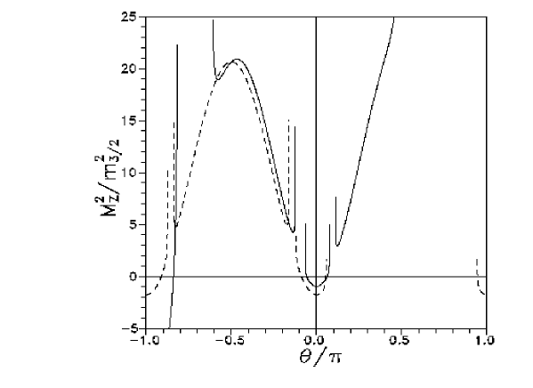
Figure 14: Dependence of $M_{Z}$ on the angle $\theta$ in the string parametrization of the soft terms shown in (20) for $\Theta_{3}=\Theta_{6}=-0.5$ (solid lines) and $\Theta_{3}=-\Theta_{6}=-0.5$ (dashed lines).

We see that $M_{Z}^{2}(\theta)$ is either negative or rather large (in units of $m_{3/2}^{2}$) and positive at the extrema, and hence not acceptable. Experimental lower bounds on the masses of superpartners imply that the scale of supersymmetry breaking measured by $m_{3/2}$ must be rather big compared to the weak scale. From a phenomenological point of view, the interesting regions of the parameter space are only those which give positive but rather small values of $M_{Z}^{2}$. Unfortunately, $\Delta_{\sin\theta}$ is never very small in such regions.

We have checked this by a numerical calculation. We have scanned the ($\theta$, $\Theta_{3}$, $\Theta_{6}$) parameter space looking for solutions with $M_{Z}^{2}$ between 0 and $m_{3/2}^{2}$ and with $M_{A}>0.6M_{Z}$. Such solutions exist only in quite a small part of the ($\Theta_{3}$, $\Theta_{6}$) parameter space. Moreover, they give very small values of $\tan\beta$ (quite close to 1), and have $\Delta_{\sin\theta}$ always well above 100. Thus, we conclude that the parametrization (20) cannot solve the fine-tuning problem.

A search for more attractive models for soft terms, perhaps guided by the phenomenological discussion of Section 5, is certainly very important.

7 Large-$\tan\beta$ Region

In this Section we update the status of scenarios with (at least approximate) $t-b-\tau$ Yukawa coupling unification [41, 42] and discuss their fine-tuning aspects. Such a possibility is realized, for instance, in $SO(10)-$type models. For $m_{t}=175$ GeV, $t-b-\tau$ unification predicts large values of $\tan\beta$: $\tan\beta\approx 50$, and the Higgs boson mass $M_{h}\stackrel{{\scriptstyle>}}{{{}_{\sim}}}110$ GeV. Clearly, if the Higgs boson is not found at LEP 2, the phenomenological relevance of the large $\tan\beta$ region will be accentuated.

Phenomenological properties of the large $\tan\beta$ region are well understood [10, 35, 36, 43, 44]. Important aspects are the breaking of the electroweak symmetry and supersymmetric one-loop corrections to the bottom quark mass and to $b\rightarrow s\gamma$ decay. To organize our discussion, let us begin with exact $t-b-\tau$ unification of Yukawa couplings in the minimal supergravity model. The results of Section 5 can be readily used to conclude that it is not a realistic scenario [36]. It is sufficient to observe that, in the parameter space constrained by requiring proper electroweak symmetry breaking, it is impossible to obtain sufficiently small one-loop supersymmetric corrections to the $b$-quark mass for stop masses up to ${\cal O}(10$ TeV) (as can be estimated from (10). The problem is even worse if we try to be consistent with $b\rightarrow s\gamma$ decay.

The question of some interest is how far we have to depart from exact unification of all three couplings in the minimal supergravity model to obtain a more realistic parameter space. One way of answering this question is to impose $b-\tau$ unification, and to study the minimal values of the stop masses and of the fine-tuning measure $\Delta_{0}$ which are necessary to satisfy all the remaining constraints, as a function of $\tan\beta$. This is shown in Fig. 7a and 7b, respectively, requiring the correct value of the $b$-quark mass and, optionally, the correct $BR(b\rightarrow s\gamma)$. As we discussed in Section 4, the prediction for the latter can be modified by a departure from the minimal supergravity model that admits some flavour structure in the stop mass matrices. We see from Fig. 7a that correct $M_{b}$ requires $M_{\tilde{t}_{2}}\sim 0.75(1.7)$ TeV for $\tan\beta$=45 without (with) the $b\rightarrow s\gamma$ constraint included. The corresponding values of $\Delta_{0}$ are 170 and 35 respectively. For $m_{t}=175$ GeV, $\tan\beta$=45 corresponds to $Y_{t}/Y_{b}\approx 1.6$ (for $M_{\tilde{t}_{i}}\sim 1$ TeV). The origin of all these results is the extremely constraining role played by electroweak symmetry breaking in the minimal supergravity model with $Y_{t}\approx Y_{b}$. In the limit $Y_{t}=Y_{b}$, the two soft Higgs boson masses $m^{2}_{H_{1}}$ and $m^{2}_{H_{2}}$ run almost in parallel, and electroweak symmetry breaking occurs only for very large values of $M_{1/2}$ and $\mu$.

It has been pointed out in [44] that a qualitatively new situation appears in the large $\tan\beta$ scenario if we relax the universality of the Higgs-doublet soft mass parameters [45, 46, 44]. This is because the correlation $\mu\gg M_{1/2}$ is no longer necessary for proper electroweak symmetry breaking, and one obtains solutions with $\mu\sim M_{1/2}\sim{\cal O}(M_{Z})$: as discussed in [44], the hierachy $m^{2}_{H_{1}}\gg m^{2}_{H_{2}}\stackrel{{\scriptstyle>}}{{{}_{\sim}}}m^{2}_{0}$ is necessary for this. In consequence, in this scenario the supersymmetric loop corrections (10) to $m_{b}(M_{Z})$ can be small. It is, therefore, interesting to repeat the analysis in this case. Since it is easy to obtain acceptable physical $M_{b}$, even for $Y_{t}=Y_{b}=Y_{\tau}$, we restrict our analysis to this case. We study the case $\tan\beta=50$ and impose $M_{b}=4.8\pm 0.2$ GeV, i.e., $2.72-3.16$ GeV for $m_{b}(M_{Z})$.

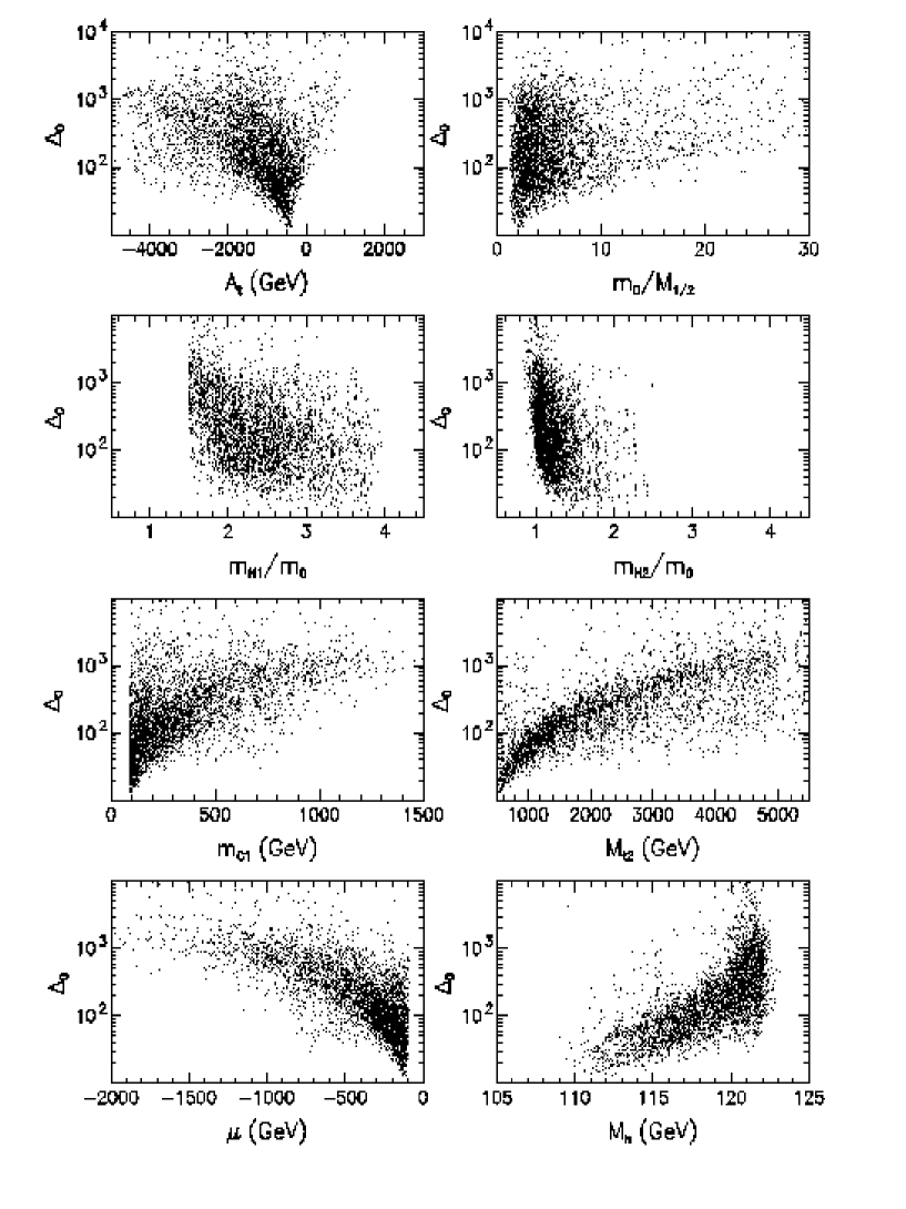
Figure 15: The price of fine tuning for $\tan\beta=50$ and $t-b-\tau$ Yukawa coupling unification, as a function of various variables in models with non-universal Higgs boson masses. The $b\rightarrow s\gamma$ constraint is not included.

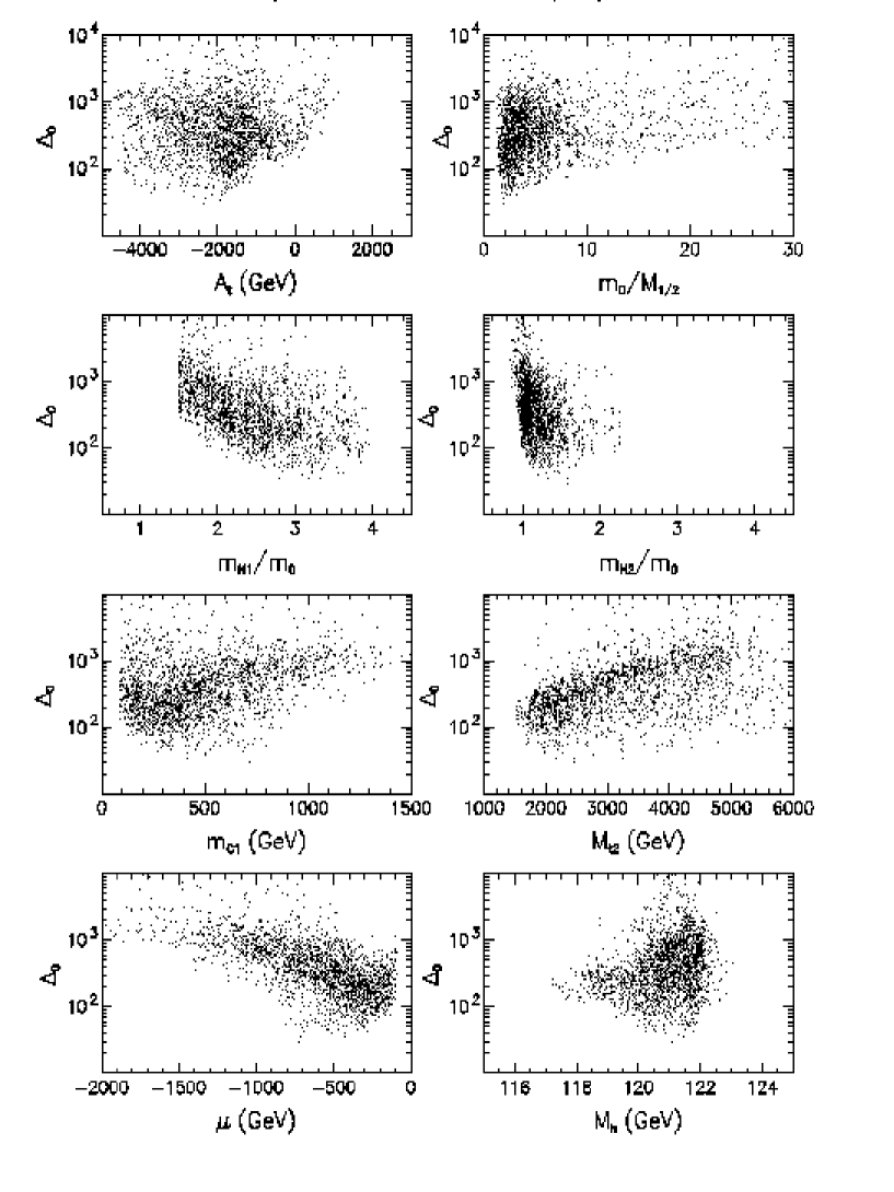
Figure 16: The same as in Fig. 15, but with the $b\rightarrow s\gamma$ constraint included.

In Fig. 15 we show some results for $\Delta_{0}$ as a function of several mass parameters, with all the constraints included except for $b\rightarrow s\gamma$. Only $\mu<0$ is possible since, as is clear from Fig. 5a, only negative one-loop supersymmetric corrections are compatible with the correct bottom-quark mass. Moreover, the correction has to be small enough and, therefore, $A_{t}$ tends to be negative and squarks must be relatively heavy. Due to the hierachy $m^{2}_{H_{1}}\gg m^{2}_{0}$, the pseudoscalar $A^{0}$ is heavy enough to assure a small amount of fine tuning : $\Delta_{0}\sim 10$ is possible. This result makes the large $\tan\beta$ region quite acceptable from the naturalness point of view.

If we insist on being consistent with $b\rightarrow s\gamma$ decay, the fine-tuning price increases to $\Delta\stackrel{{\scriptstyle>}}{{{}_{\sim}}}40$, as seen in Fig. 16. This happens for reasons similar to those discussed for $\tan\beta=30$ in the minimal model, and the discussion at the end of Section 4 applies unchanged to the present case.

Finally, we remark that the non-universal Higgs boson masses discussed here give solutions with higgsino-like neutralinos. Thus, such scenarios generically lead to a rather low neutralino dark matter density [30].

8 Conclusions

Comparing the situation before and after LEP, the fine-tuning price in the minimal supergravity model has increased significantly, largely as a result of the unsuccessful Higgs boson search. Comparing different values of $\tan\beta$, we find that naturalness favours an intermediate range. Fine tuning increases for small values because of the lower limit on the Higgs mass, in particular, and increases for large values because of the difficulty in assuring correct electroweak symmetry breaking.

Additional theoretical assumptions may have a significant impact on the fine-tuning price. For example, requiring $b-\tau$ Yukawa-coupling unification would increase the price significantly at intermediate $\tan\beta$, whereas imposing certain linear correlations between mass parameters could diminish it substantially. One particular class of models imposing such have been motivated from string constructions: unfortunately, those currently available do not seem to reduce the fine-tuning price significantly, so naturalness considerations do not favour these models to any substantial extent. However, the search for realistic theoretical models which do reduce the fine-tuning price is a very interesting issue.

We have found that $b\rightarrow s\gamma$ decay is a potentially important constraint for large $\tan\beta$, but we would argue that it should be regarded as optional. The flavour structure of squark couplings could differ from those of the quarks, and there are no direct FCNC limits on flavour violation among superpartners of the up quarks.

A final comment concerns the region of very large $\tan\beta$. In this case, the fine-tuning price can be reduced quite substantially by allowing non-universal soft mass parameters for the Higgs bosons. This is in contrast to the situation at lower $\tan\beta$, where non-universal mass parameters do not reduce the price significantly.

We re-emphasize that naturalness is subjective criterion, based on physical intuition rather than mathematical rigour. Nevertheless, it may serve as an important guideline that offers some discrimination between different theoretical models and assumptions. As such, it may indicate which domains of parameter space are to be preferred. However, one should be very careful in using it to set any absolute upper bounds on the spectrum. We think it safer to use relative naturalness to compare different scenarios, as we have done in this paper.

Acknowledgments.

The work of P.H.Ch. has been partly supported by the Polish State Committee for Scientific Research grant 2 P03B 030 14 (1998-1999) and by the U.S.-Polish Maria Skłodowska-Curie Joint Fund II (MEN/DOE-96-264). The work of M.O. was supported by the Polish State Committee for Scientific Research grant 2 P03B 030 14 (1998-1999) and by the Sonderforschungsbereich 375-95 für Astro-Teilchenphysik der Deutschen Forschungsgemeinschaft. The work of S.P. has been supported by the Polish State Committee for Scientific Research grant 2 P03B 030 14 (1998-1999).

References

-
[1]
J. Ellis, S. Kelley and D.V. Nanopoulos, Phys. Lett.
B249 (1990) 441 and B260 (1991) 131;
C. Giunti, C.W. Kim and U.W. Lee, Mod. Phys. Lett. A6 (1991) 1745;
U. Amaldi, W. de Boer and H. Fürstenau, Phys. Lett. B260 (1991) 447;
P. Langacker and M. Luo, Phys. Rev. D44 (1991) 817. - [2] P.H. Chankowski, Z. Płuciennik and S. Pokorski, Nucl. Phys. B439 (1995) 23.
-
[3]
J. Ellis, G.L. Fogli and E.Lisi, Phys. Lett. B389 (1996) 321 and references therein;
P.H. Chankowski and S. Pokorski, Phys. Lett. B356 (1995) 307 and hep-ph/9509207. -
[4]
D. Ward, Plenary talk at the Europhysics
Conference on High-Energy Physics, Jerusalem, August 1997;
D. Reid, Talk at the XXXIIIth Rencontres de Moriond on Electroweak Interactions and Unified Theories, Les Arcs, France, March 1998;
LEP Electroweak Working Group, CERN report LEPEWWG/98-01. -
[5]
L. Maiani, Proceedings Summer School on Particle
Physics, Gif-sur-Yvette, 1979 (IN2P3, Paris, 1980), p.3;
G. ’t Hooft, in Recent Developments in Field Theories, eds. G. ’t Hooft et al., (Plenum Press, New York, 1980);
E. Witten, Nucl. Phys. B188 (1981) 513;
R.K. Kaul, Phys. Lett. 109B (1982) 19. - [6] P.H. Chankowski, J. Ellis and S. Pokorski, Phys. Lett. B423 (1998) 327.
- [7] J. Ellis, K. Enqvist, D.V. Nanopoulos and F. Zwirner, Nucl. Phys. B276 (1986) 14.
-
[8]
R. Barbieri and G.-F. Giudice, Nucl. Phys. B306
(1988) 63;
S. Dimopoulos and G.-F. Giudice, Phys. Lett. B357 (1995) 573. -
[9]
G.W. Anderson and D.J. Castaño, Phys. Lett.
B347 (1995) 300, Phys. Rev. D52 (1995) 1693
and D53 (1996) 2403;
K.L. Chan, U. Chattopadhyay and P. Nath, hep-ph/9710473;
P. Ciafaloni and A. Strumia, Nucl. Phys. B494 (1997) 41. -
[10]
M. Olechowski and S. Pokorski, Nucl. Phys. B404
(1993) 590;
B. de Carlos and J.A. Casas, Phys. Lett. B309 (1993) 320. - [11] R. Barbieri and A. Strumia, preprint IFUP-TH-4-98, (hep-ph/9801353).
-
[12]
ALEPH Collaboration, ALEPH 98-029 CONF 98-017;
DELPHI Collaboration, talk by K. Moenig, LEPC Meeting, CERN, March 31, 1998;
M. Acciarri (L3 Collaboration) et al., preprint CERN-EP/98-052;
OPAL Physics Note PN340, March 1998;
V. Ruhlmann-Kleider, Talk at the XXXIIIth Rencontres de Moriond on QCD and High-Energy Interactions, Les Arcs, March 1998;
M. Felcini, Talk at the 1st European Meeting From the Planck Scale to the Electroweak Scale, Kazimierz, Poland, May 1998. - [13] CLEO Collaboration, preprint CLEO CONF 98-17 submitted to the XXIXth International Conference on High-Energy Physics, Vancouver, B.C., Canada, paper ICHEP98 101.
-
[14]
M.S. Chanowitz, J. Ellis and M.K. Gaillard,
Nucl. Phys. B128 (1977) 506;
A.J. Buras, J. Ellis, M.K. Gaillard and D.V. Nanopoulos, Nucl. Phys B135 (1978) 66. - [15] M. Carena, M. Olechowski, S. Pokorski and C.E.M. Wagner, Nucl. Phys. B419 (1994) 213.
- [16] M. Carena, P.H. Chankowski, M. Olechowski, S. Pokorski and C.E.M. Wagner, Nucl. Phys. B491 (1997) 103.
-
[17]
R. Hempfling, U.C. Santa Cruz Ph. D. thesis, preprint
SCIPP 92/28 (1992);
J. Ellis, G. Ridolfi and F. Zwirner, Phys. Lett. 257B (1991) 83 and Phys. Lett. 262B (1991) 477;
J.L. Lopez, D.V. Nanopoulos, Phys. Lett. 266B (1991) 397. -
[18]
M. Carena, J.-R. Espinosa, M. Quiros and C.E.M. Wagner,
Phys. Lett. 355B (1995) 209;
M. Carena, M. Quiros and C.E.M. Wagner, Nucl. Phys. B461 (1996) 407. - [19] M. Carena, P.H. Chankowski, S. Pokorski and C.E.M. Wagner, preprint FERMILAB-PUB-98-146-T, hep-ph/9805349.
- [20] G. Kane, C.Kolda, L. Roszkowski and J.D. Wells, Phys. Rev. D 49 (1994) 6173.
- [21] G. Altarelli, R. Barbieri and F. Caravaglios, Phys. Lett. B314 (1993) 357.
- [22] J. Ellis, G. Fogli and E. Lisi, Phys. Lett. B324 (1994) 173.
-
[23]
P.H. Chankowski and S. Pokorski, Phys. Lett. B366 (1996) 188 and preprint SCIPP/97-19,
IFT/97-13, hep-ph/9707497, to appear in Perspectives on Supersymmetry,
ed. G.L. Kane (World Scientific, Singapore);
see also P.H. Chankowski, preprint IFT/97-18, hep-ph/9711470, to appear in Proceedings of the International Workshop on Quantum Effects in the MSSM, Barcelona, September 1997. - [24] W. de Boer, A. Dabelstein, W.F.L. Hollik and W. Mösle, preprint IEKP-KA-96-08, hep-ph/9609209.
-
[25]
Open session of the LEP experiments Committee,
Nov. 11th, 1997:
P. Charpentier, representing the DELPHI collaboration,
http://wwwinfo.cern.ch/ charpent/LEPC/;
A. Honma, representing the OPAL collaboration,
http://www.cern.ch/Opal/;
P. Dornan, representing the ALEPH collaboration;
M. Pohl, representing the L3 collaboration,
http://hpl3sn02.cern.ch/conferences/talks97.html. -
[26]
C. Greub, T. Hurth and D. Wyler,
Phys. Lett. B380 (1996) 385 and
Phys. Rev. D54 (1996) 3350;
K. Chetyrkin, M. Misiak and M. Münz, Phys. Lett. B400 (1997) 206. -
[27]
K. Adel and Y.P. Yao, Phys. Rev. D49 (1994)
4945;
M. Ciuchini, G. Degrassi, P. Gambino and G.-F. Giudice, preprint CERN-TH-97-279, hep-ph/9710335;
P. Ciafaloni, A. Romanino and A. Strumia, Nucl. Phys. B524 (1998) 361. - [28] R. Barbieri and G.-F. Giudice, Phys. Lett. B309 (1993) 86.
- [29] M. Misiak, S. Pokorski and J. Rosiek, in Heavy Flavours II, eds. A.J. Buras, M. Lindner, Advanced Series on Directions in High-Energy Physics, World Scientific, Singapore (hep-ph/9703442).
-
[30]
J. Ellis, T. Falk, K.Olive and M. Schmitt,
Phys. Lett. B413 (1997) 335;
J. Ellis, T. Falk, G. Ganis, K.A. Olive and M. Schmitt, hep-ph/9801445. - [31] P.H. Chankowski, Phys. Rev. D41 (1990) 2877.
- [32] J. Rosiek, Phys. Rev. D41 (1990) 3464.
- [33] T. Blazek and S. Raby, Phys. Lett. B392 (1997) 371 and hep-ph/9712255.
- [34] M. Beneke, Talk at the XXXIIIth Rencontres de Moriond on Electroweak Interactions and Unified Theories, Les Arcs, France, March 1998, preprint CERN-TH/98-202, hep-ph/9806429.
-
[35]
L.J. Hall, R. Ratazzi and U. Sarid, Phys. Rev.
D50 (1994) 7048;
R. Hempfling, Phys. Rev. D49 (1994) 6168. - [36] M. Carena, M. Olechowski, S. Pokorski and C.E.M. Wagner, Nucl. Phys. B426 (1994) 269.
-
[37]
K.T. Matchev and D.M. Pierce, preprint SLAC-PUB-7821,
(hep-ph/9805275);
D.M. Pierce, Talk given at the SUSY 98 Inernational Conference, Oxford, U.K., 1998. - [38] F. Gabbiani, E. Gabrielli, A. Masiero and L. Silvestrini, Nucl. Phys.B447 (1996) 321.
- [39] F. Borzumati, M. Olechowski and S. Pokorski, Phys. Lett. B349 (1995) 311.
- [40] A. Brignole, L.E. Ibáñez, C. Muñoz and C. Scheich, Z. Phys. C74 (1997) 157.
-
[41]
T. Banks, Nucl. Phys. B303 (1988) 172;
M. Olechowski and S. Pokorski, Phys. Lett. B214 (1988) 393;
G.F. Giudice and G. Ridolfi, Z. Phys. C41 (1988) 447. -
[42]
B. Anantharayan, G. Lazarides and Q. Shafi, Phys. Rev.
D44 (1991) 1631;
S. Dimopoulos, L.J. Hall and S. Raby Phys. Rev. Lett 68 (1992) 1984 and Phys. Rev. D45 (1992) 606. -
[43]
M. Drees and M.M. Nojiri, Nucl. Phys. B369
(1992) 54;
B. Ananthanarayan, G. Lazarides and Q. Shafi, Phys. Lett. B300 (1993) 245. - [44] M. Olechowski and S. Pokorski, Phys. Lett. B344 (1995) 201.
- [45] N. Polonsky and A. Pomarol, Phys. Rev. Lett. 73 (1994) 2292.
- [46] D. Matalliotakis and H.P. Nilles, Nucl. Phys. B435 (1995) 115.