Pattern of Chiral Symmetry Restoration at Finite Temperature
in A Supersymmetric Composite Model

Abstract

The structure of chiral symmetry restorations at finite temperature is thoroughly investigated in the supersymmetric Nambu-Jona-Lasinio model with a soft supersymmetry breaking term. It is found that the broken chiral symmetry at vanishing temperature is restored at sufficiently high temperature in two patterns, i. e., the first order and second order phase transition depending on the choice of the coupling constant $G$ and the supersymmetry breaking parameter $\Delta$. The critical curves expressing the phase boundaries in the $G-\Delta$ plane are completely determined and the dynamically generated fermion mass is calculated as a function of temperature.

The supersymmetry is an essential ingredient of unified field theories for elementary particles so that it is worth trying to study a supersymmetric version of composite Higgs models such as Technicolor model. We shall consider a supersymmetric composite model in the present communication with an interest in the early universe and take into account finite temperature effects. As a prototype of the composite model we pick up the Nambu-Jona-Lasinio (NJL) model which is known to be useful to investigate the mechanism of the dynamical symmetry breaking [1]. The supersymmetric version of the NJL model is easily constructed. Unfortunately, however, in the supersymmetric NJL model the chiral symmetry is strongly protected to keep the boson-fermion supersymmetry (SUSY) and hence the dynamical chiral symmetry breaking does not take place [2]. If a soft SUSY breaking term is added to the SUSY NJL Lagrangian, the dynamical breakdown of the chiral symmetry is brought about for sufficiently large SUSY breaking parameter $\Delta$ [3]. The reason for this is simple: The large $\Delta$ implies the large effective mass of the scalar components of the superfields so that quantum effects due to the scalar components get suppressed compared with that of the spinor components. Thus the model becomes closer to the original NJL model which allows the dynamical fermion mass generation. Stating the same substance in a different way we realize that the boson by acquiring its mass term forces supersymmetry to make balance so that the fermion mass is generated dynamically.

The SUSY NJL model with soft SUSY breaking is useful to study the mechanism of the dynamical chiral symmetry breaking within the framework of supersymmetry. If we take the model seriously as a prototype of the unified field theory, it is natural to extend the argument to take into account circumstances of the finite temperature and spacetime-curvature as in the early universe. It should, however, be noted that SUSY is not a good symmetry for finite temperature [4]. This fact may discourage studies of SUSY models at finite temperature. In our argument we consider the supersymmetry of the model in the strict sense only at vanishing temperature and focus our attention on the dynamical breaking of the chiral symmetry in the same model at finite temperature. The breaking of SUSY at finite temperature is kinematical since it is caused essencially by the difference of the statistical distribution functions for bosons and fermions.

A natural SUSY extension of the NJL model is characterized by the following Lagrangian [2],

$${\cal L}_{SNJL}=\int d^{4}\theta [\bar{\Phi}_{+}\Phi_{+}+\bar{\Phi}_{-}\Phi_{-}+\frac{G}{N}\ \Phi_{+}\Phi_{-}\bar{\Phi}_{+}\bar{\Phi}_{-}$$ (2)

$$-\Delta^{2}\theta^{2}\bar{\theta}^{2}(\bar{\Phi}_{+}\Phi_{+}+\bar{\Phi}_{-}\Phi_{-})],$$

where $d^{4}\theta=d^{2}\theta d^{2}\bar{\theta}$. The chiral superfield ${\Phi}_{\pm}$ is represented by component scalar ($\phi_{\pm}$) and spinor ($\psi_{\pm}$) fields and auxiliary field $F_{\pm}$ so that $\Phi_{\pm}(y)=\phi_{\pm}(y)+\sqrt{2}\theta\psi_{\pm}(y)+F_{\pm}(y)\theta^{2}$ with $y=x+i\theta\sigma^{\mu}\bar{\theta}$. The chiral superfields $\Phi_{+}$ and $\Phi_{-}$ belong to the multiplet $N$ and $\bar{N}$ in $SU(N)$ respectively. Note that a soft SUSY breaking term is introduced in Eq. (2) following Buchmueller and Ellwanger [3].

In the following arguments it is convenient to introduce auxiliary chiral superfields $H$ and $S$ and use a Lagrangian equivalent to Eq. (2)

$${\cal L} = \int d^{4}\theta[(\bar{\Phi}_{+}\Phi_{+}+\bar{\Phi}_{-}\Phi_{-})(1-\Delta^{2}\theta^{2}\bar{\theta}^{2})+\frac{N}{G}\bar{H}H]$$ (3)

$$+ [\int d^{2}\theta\ (\frac{N}{G}HS-S\Phi_{+}\Phi_{-})+h.c.].$$ (4)

Written in terms of component fields the Lagrangian takes the following form where we have kept only relevant terms for calculating our effective potential in the leading order of the $1/N$ expansion:

$${\cal L} = -\bar{\phi}_{+}(\Box+|\phi_{S}|^{2}+\Delta^{2})\phi_{+}-\bar{\phi}_{-}(\Box+|\phi_{S}|^{2}+\Delta^{2})\phi_{-}$$ (6)

$$+\bar{\Psi}(i\partial_{\mu}\gamma^{\mu}-\sigma+i\gamma_{5}\pi)\Psi-\frac{N}{G}|\phi_{S}|^{2}.$$

The field $\phi_{S}$ is related to the ordinary scalar ($\sigma$) and pseudoscalar ($\pi$) field such that $\phi_{S}=\sigma+i\pi$, and $\Psi=(\psi_{+},\bar{\psi}_{-})^{T}$.

We would like to calculate the effective potential for Lagrangian (6) in the leading order of the $1/N$ expansion at finite temperature. We adopt the Matsubara formalism [5] to introduce temperature effects in our calculation of the effective potential. We simply replace the integral in energy variable by the summation where we apply the periodic boundary condition for boson fields and the anti-periodic boundary condition for fermion fields respectively. The calculation of the effective potential is essentially the same as the one described in our previous paper [6]. The summation can be easily performed and after some algebra the following result is obtained,

$$V(|\phi_{S}|^{2})=V_{0}(|\phi_{S}|^{2})+V_{\beta}(|\phi_{S}|^{2}),$$ (7)

where $V_{0}(|\phi_{S}|^{2})$ is the effective potential for vanishing temperature,

$$V_{0}(|\phi_{S}|^{2}) = \frac{|\phi_{S}|^{2}}{G}+2\int\frac{d^{D-1}k}{(2\pi)^{D-1}}(\ \sqrt{k^{2}+|\phi_{S}|^{2}+\Delta^{2}}$$ (9)

$$-\sqrt{k^{2}+|\phi_{S}|^{2}}-\sqrt{k^{2}+\Delta^{2}}+\sqrt{k^{2}}\ ),$$

which agrees with the one obtained by performing the $k_{0}$ integration after Wick rotation in the effective potential given at vanishing temperature, and $V_{\beta}(|\phi_{S}|^{2})$ is the temperature dependent part of the effective potential that is given by

$$V_{\beta}(|\phi_{S}|^{2}) = -\frac{4}{\beta}\int\frac{d^{D-1}k}{(2\pi)^{D-1}}\ln(\frac{1+e^{-\beta\sqrt{k^{2}+|\phi_{S}|^{2}}}}{1+e^{-\beta\sqrt{k^{2}}}}$$ (11)

$$\hskip 28.45274pt\times\frac{1-e^{-\beta\sqrt{k^{2}+\Delta^{2}}}}{1-e^{-\beta\sqrt{k^{2}+|\phi_{S}|^{2}+\Delta^{2}}}}),$$

where $D$ is the space-time dimension (Although $D=4$, we keep $D$ to be arbitrary in Eqs. (9) and (11) for later convenience), $\beta$ is the inverse of the temperature $T$ in unit of $k_{B}=1$ with $k_{B}$ the Boltzmann constant. Note that the effective potential (7) is normalized so that $V(0)=0$.

It is easy to see that the effective potential (7) reduces to $V_{0}(|\phi_{S}|^{2})$ in the zero temperature limit $\beta\to\infty$. If we let $\Delta\to 0$ in the zero temperature effective potential (9), we are left only with the tree term as is expected by the boson-fermion cancellation in the SUSY model. In the SUSY limit $\Delta\to 0$ the finite temperature effective potential (11) still retains the term of quantum corrections which is composed of the bosonic and fermionic statistical distribution functions. This result reflects the well-known fact that supersymmetry is not a good symmetry at finite temperature [4]. At sufficiently low temperature both the Fermi-Dirac and Bose-Einstein distribution function $1/(\exp{\beta\sqrt{k^{2}+|\phi_{S}|^{2}}\pm 1})$ are well approximated by the Maxwell-Boltzmann distribution function $\exp(-\beta\sqrt{k^{2}+|\phi_{S}|^{2}})$ and hence the quantum correction term in Eq. (7) disappears. Thus supersymmetry is a good symmetry not only at zero temperature but also in the low temperature region.

Although the phase structure of our model at finite temperature is studied by direct numerical estimates of the effective potential (7), it is more convenient to deal with the gap equation $V^{\prime}(|\phi_{S}|^{2})=0$ where the prime denotes the differenciation with respect to $|\phi_{S}|^{2}$ : $V^{\prime}(|\phi_{S}|^{2})=\partial V/\partial|\phi_{S}|^{2}$,

$$\frac{1}{G} - \int\frac{d^{D-1}k}{(2\pi)^{D-1}}(\frac{1}{\sqrt{k^{2}+|\phi_{S}|^{2}}}-\frac{1}{\sqrt{k^{2}+|\phi_{S}|^{2}+\Delta^{2}}})$$ (14)

$$+2\int\frac{d^{D-1}k}{(2\pi)^{D-1}}[\ \frac{1}{\sqrt{k^{2}+|\phi_{S}|^{2}}}\frac{1}{e^{\beta\sqrt{k^{2}+|\phi_{S}|^{2}}}+1}$$

$$-\frac{1}{\sqrt{k^{2}+|\phi_{S}|^{2}+\Delta^{2}}}\frac{1}{e^{\beta\sqrt{k^{2}+|\phi_{S}|^{2}+\Delta^{2}}}-1}\ ]=0.$$

In order to see the situation as clearly as possible we start with the discussion in the case $D=3$ where the gap equation (14) after performing the integration is much simpler than the one for $D=4$ and there is no divergence in the integration in Eq. (14). The gap equation for $D=3$ is obtained in an analytical form by performing the integration in Eq. (14):

$$\frac{2\pi}{G}-\sqrt{|\phi_{S}|^{2}+\Delta^{2}}+\sqrt{|\phi_{S}|^{2}}+\frac{2}{\beta}\ln{\frac{1+e^{-\beta\sqrt{|\phi_{S}|^{2}}}}{1-e^{-\beta\sqrt{|\phi_{S}|^{2}+\Delta^{2}}}}}=0.$$ (15)

By numerical inspections we find that Eq. (15) allows at most two nontrivial solutions for $|\phi_{S}|^{2}$ depending on the choice of parameters $G$, $\Delta$ and $\beta$. Thus the effective potential (7) with $D=3$ may have zero, one and two extremum (extrema) respectively. Hence, when the temperature $1/\beta$ is increased, we will have possibilities of experiencing no phase transition, the 2nd order phase transition and the 1st order phase transition.

The effective potential $V(|\phi_{S}|^{2})$ for $D=3$ is calculated analytically such that

$$V(|\phi_{S}|^{2}) = \frac{|\phi_{S}|^{2}}{G}+\frac{1}{3\pi}[|\phi_{S}|^{3}+\Delta^{3}-(|\phi_{S}|^{2}+\Delta^{2})^{3/2}]$$ (17)

$$+V_{\beta}(|\phi_{S}|^{2})_{D=3},$$

where we have suppressed writing explicitly the temperature dependent term (the last term on the right hand side of Eq. (17)) which is rather lengthy and can be expressed by using the polylogarithms.

At vanishing temperature the chiral symmetry in the model is broken [3] if sufficiently large is the parameter $\Delta$ appearing in the soft SUSY breaking term. In fact by observing the behavior of the gap equation $V_{0}^{\prime}(|\phi_{S}|^{2})=0$ we can confirm the statement. In three dimensions for vanishing temperature $\beta\to\infty$ the last term on the left hand side of Eq. (15) disappears and we see that only one nontrivial solution for $|\phi_{S}|^{2}$ exists when $2\pi/G<\Delta$. The curve on the $G-\Delta$ plane given by the equation

$$G\Delta/(2\pi)=1$$ (18)

divides the whole $G-\Delta$ plane into two regions which represent the unbroken and broken chiral symmetry respectively.

If the parameters $G$ and $\Delta$ are kept in the unbroken region, we remain in the unbroken region when temperature is increased. If the parameters $G$ and $\Delta$ are in the broken region, we experience the chiral symmetry restoration as temperature gets high enough. This situation is easily confirmed by observing the gap equation (15) and the effective potential (17). In the present situation there are two types of the chiral symmetry restoration : the first-order and second-order phase transition. These two cases can be distinguished from each other by the conditions $V^{\prime}(0)=0,V^{\prime\prime}(0)<0$ and $V^{\prime}(0)=0,V^{\prime\prime}(0)>0$ respectively. Hence the condition that $|\phi_{S}|^{2}=0$ be a point of inflection for the effective potential, $V^{\prime}(0)=V^{\prime\prime}(0)=0$, divides these two cases and gives a curve on the $G-\Delta$ plane. The curve is the critical curve on the $G-\Delta$ plane which divides the region of the broken phase into the regions of the first and second order phase transition. Written in parameters $G$ and $\Delta$ the condition $V^{\prime}(0)=V^{\prime\prime}(0)=0$ reads

$$\frac{2\pi}{G\Delta}=1-\frac{2}{\beta\Delta}\ln{\frac{2}{1-e^{-\beta\Delta}}},$$ (19)

$$\beta\Delta/2=\coth(\beta\Delta/2).$$ (20)

Here $\beta\Delta/2$ is determined by Eq. (20) and is equal to 1.19968. The critical curve distinguishing the second order phase transition from the first order one is given by the equation obtained by substituting the above value for $\beta\Delta/2$ in Eq. (19), i.e.,

$$G\Delta/(2\pi)=2.91631.$$ (21)

The whole $G-\Delta$ plane is divided by two hyperbolas (18) and (21) into three regions which correspond to the unbroken, broken (2nd order) and broken (1st order) region respectively as shown in Fig. 1. Note here that as can be seen in Eq. (17) the effective potential for $D=3$ reduces to that of the ordinary NJL model by letting $\Delta\to\infty$. The physical reason for this result is simple: In the limit of large $\Delta$ the scalar components of the superfield carry a large effective mass and decouple from the spinor components leaving only the contribution of the NJL fermions. It should, however, be remarked that the gap equation (15) diverges as $\Delta\to\infty$. This result corresponds exactly to the fact that the gap equation for the ordinary NJL model diverges linearly for $D=3$. In fact it is given by

$$\frac{2\pi}{G}=\Lambda-\sqrt{|\phi_{S}|^{2}}-\frac{2}{\beta}\ln(1+e^{-\beta\sqrt{|\phi_{S}|^{2}}})$$ (22)

and corresponds to Eq. (15) with large $\Delta$ replaced by $\ Lambda$. In the ordinary NJL model for three dimensions the bare coupling constant $G$ is to be kept small for large $\Lambda$. This fact precisely reflects the property that $G$ gets smaller as $\Delta$ becomes larger along the critical curve.

We then go over to the case of the four dimensional space-time. For $D=4$ the situation is almost the same as in $D=3$. The main difference comes from the presence of the divergence for $D=4$ in the integration of Eqs.(7) and (14). We regularize the divergence by introducing the three dimensional cut-off $\Lambda$ in the momentum integration. The effective potential for $D=4$ at vanishing temperature $V_{0}(|\phi_{S}|^{2})$ is calculated analytically while the temperature dependent part of the effective potential $V_{\beta}(|\phi_{S}|^{2})$ is estimated numerically. In these calculations all the parameters in the model are scaled by the cut-off $\Lambda$. By direct numerical estimates we find that the effective potential (7) with $D=4$ represents the chiral symmetry restoration as temperature gets high enough. In Fig. 2 (a) and (b) we see that the chiral symmetry restoration is of the 2nd as well as 1st order phase transition depending on the choice of the parameters $G$ and $\Delta$ (In our previous paper the existance of the 2nd order phase transition was overlooked [7]).

The gap equation $\partial V/\partial|\phi_{S}|^{2}=0$ reads

$$\frac{1}{2\alpha} - \sqrt{1+x}+\sqrt{1+x+\delta}-(x+\delta)\ln\frac{1+\sqrt{1+x+\delta}}{\sqrt{x+\delta}}$$ (24)

$$+x\ln\frac{1+\sqrt{1+x}}{\sqrt{x}}+\frac{4\pi^{2}}{\Lambda^{2}}\frac{\partial V_{\beta}(|\phi_{S}|^{2})_{D=4}}{\partial|\phi_{S}|^{2}}=0,$$

where $\alpha$, $\delta$ and $x$ are defined by $\alpha=G\Lambda^{2}/(8\pi^{2}),\delta=\Delta^{2}/\Lambda^{2},x=|\phi_{S}|^{2}/\Lambda^{2}$. For $\beta\to\infty$ the last term on the left hand side in Eq. (24) drops out leaving only temperature independent terms and we have the gap equation at zero temperature. It is not difficult to show that Eq. (24) without the temperature dependent term allows a nontrivial solution for $x$ when the parameters $\alpha$ and $\delta$ satisfy the condition,

$$\frac{1}{2\alpha}<1-\sqrt{1+\delta}+\delta\ln\frac{1+\sqrt{1+\delta}}{\sqrt{\delta}}.$$ (25)

Thus the dynamical fermion mass is generated and the chiral symmetry is broken dynamically at vanishing temperature if the above inequality is satisfied. The boundary of the region given by Eq. (25) in the $\alpha-\delta$ plane is the critical curve dividing the symmetric and broken phase as shown in Fig. 3.

Just in parallel with the case of $D=3$ we find three possibilities in which the gap equation (24) allows no solution, one nontrivial solution and two nontrivial solutions respectively depending on the choice of parameters $G$, $\Delta$ and $\beta$. It is easily found by observing the behaviors of the gap equation and the effective potential that there are two types of phase transitions, the first order and second order, as temperature increases. As in the case of $D=3$ the critical curve distinguishiding the region of the 1st order phase transition from the region of the 2nd order phase transition is given by solving simultaneous equations for $G$ and $\Delta$ corresponding to the following equations,

$$V^{\prime}(0)=V^{\prime\prime}(0)=0.$$ (26)

The critical curve derived from Eq. (26) is shown by a dotted line in Fig. 3.

The full and dotted line divide the whole $G-\Delta$ region into three regions of the unbroken chiral symmetry, the broken chiral symmetry with the 2nd order phase transition and the broken chiral symmetry with the 1st order phase transition respectively. The dynamical fermion mass generated by the above chiral symmetry breaking is obtained by numerically solving the gap equation (24) as is shown in Fig. 4.

One of the direct physical consequences of our approach may be found in the field of electroweak baryogenesis in early Universe [8]. In this connection it is interesting to see whether composite Higgs masses can be taken large enough to account for the present experimental observation and to construct realistic composite Higgs models for describing the baryogenesis [9]. As a physicsl application of our approach we may consider the supersymmetric $E_{6}$ GUT model [10] in which the symmetry breaking patterns can be precisely investigated by using our results. It is also interesting to note whether our results presented in the paper is subject to any change if we introduce the contribution of order $1/N$ or higher. Such calculation has been done in Ref. [11] in the case of the nonsupersymmetric NJL model in three dimensions and an extension of their result to the case of the SUSY NJL model should be straightforward. The investigation in this direction will be left for future works.

After the completion of our work we became aware of a report discussing the similar analysis as in the present paper [12]. The conclusion of Ref. [12], however, is quite different from ours.

The authors would like to thank K. Kikkawa and C. S. Lim for useful comments on supersymmetry at finite temperature and T. Inagaki, S. Mukaigawa and M. Tanabashi for enlightening discussions.

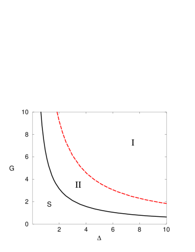
FIG. 1.: Critical curves on $G-\Delta$ plane in $D=3$: ’S’ represents the region of the parameters $G$ and $\Delta$ in which the chiral symmetry is not broken at any temperature, ’II’ represents the region of the parameters in which the broken chiral symmetry at vanishing temperature is restored at high temperature as the second order phase transition and ’I’ represents the region of the parameters in which the broken chiral symmetry at vanishing temperature is restored at high temperature as the first order phase transition.

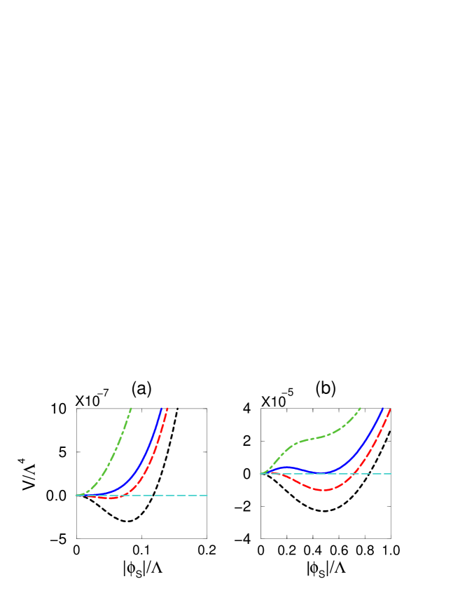
FIG. 2.: The $\beta$ dependence of the effective potential (a) for $\alpha=25$ and $\delta=0.1$ and (b) for $\alpha=90$ and $\delta=0.1$.

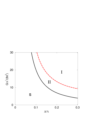
FIG. 3.: Critical curves on $G-\Delta$ plane in $D=4$: The explanation of symbols ’S’, ’II’ and ’I’ is the same as the one in Fig. 1.

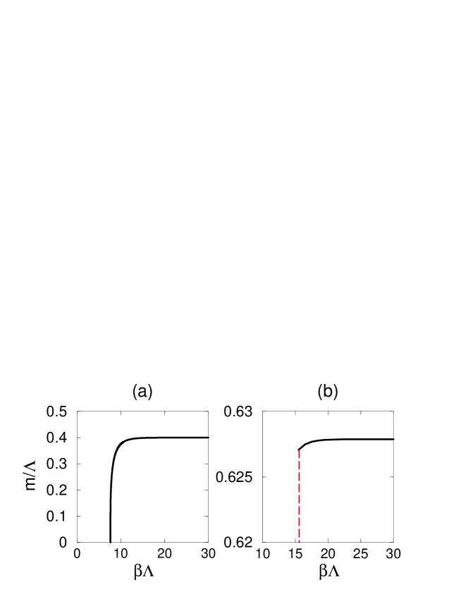
FIG. 4.: The dynamical fermion mass as a function of $\beta$ (a) for $\alpha=25$ and $\delta=0.1$ and (b) for $\alpha=90$ and $\delta=0.1$.

REFERENCES

- [1] Y. Nambu and G. Jona-Lasinio, Phys. Rev. 122(1961) 345.
- [2] W. Buchmueller and S. T. Love, Nucl. Phys. B204(1982) 213; V. Elias, D. G. C. Mckeon, V. A. Miransky and I. A. Shovkovy, Phys.Rev. D54(1996)7884; L. L. Buchbinder, T. Inagaki and S. D. Odintsov, Mod. Phys. Lett. A12(1997) 2271.
- [3] W. Buchmueller and U. Ellwanger, Nucl. Phys. B245(1984) 237.
- [4] D. Buchholtz and I. Ojima, Nucl. Phys. B498(1997) 228 and references cited therein.
- [5] T. Matsubara, Prog. Theor. Phys. 14(1955) 351.
- [6] T. Inagaki, T. Kouno and T. Muta, Intern. J. Mod. Phys. A10(1995) 2241.
- [7] J. Hashida, T. Muta and K. Ohkura, Mod. Phys. Lett. A13(1998) 1235.
- [8] J. M. Cline and G. D. Moore, Phys. Rev. Lett. 81(1998) 3315 and references cited therein.
- [9] A. I. Bochkarev, S. V. Kuzmin and M. E. Shaposhnikov, Phys. Lett. B244 (1990) 275, K. Funakubo, Prog. Theor. Phys. 96 (1996) 475; hep-ph/9809517, F. Csikor, Z. Fodor and J. Heitger, Phys.Lett. B441(1998) 354.
- [10] T. Kugo and J. Sato, Prog. Theor. Phys.91(1994)1217.
- [11] F. P. Esposito, I. A. Shovkovy and L. C. R. Wijewardhana, Phys. Rev. D58(1998) 065003.
- [12] Z. Lalak, J. Pawelczyk and S. Pokorski, Preprint MPI-Ph/93-42(1993).