hep-ph/9808251 ACT-7/98 CERN-TH/98-216 CTP-TAMU-25/98 IOA-10/1998 Neutrino Textures in the Light of Super-Kamiokande Data and a Realistic String Model

Motivated by the Super-Kamiokande atmospheric neutrino data, we discuss possible textures for Majorana and Dirac neutrino masses within the see-saw framework. The main purposes of this paper are twofold: first to obtain intuition from a purely phenomenological analysis, and secondly to explore to what extent it may be realized in a specific model. We comment initially on the simplified two-generation case, emphasizing that large mixing is not incompatible with a large hierarchy of mass eigenvalues. We also emphasize that renormalization-group effects may amplify neutrino mixing, presenting semi-analytic expressions for estimating this amplification. Several examples are then given of three-family neutrino mass textures which may also accommodate the persistent solar neutrino deficit, with different assumptions for the neutrino Dirac mass matrices. We comment on a few features of neutrino mass textures arising in models with a $U(1)$ flavour symmetry. Finally, we discuss the possible pattern of neutrino masses in a ‘realistic’ flipped $SU(5)$ model derived from string theory, illustrating how a desirable pattern of mixing may emerge. Both small- or large-angle MSW solutions are possible, whilst a hierarchy of neutrino masses appears more natural than near-degeneracy. This model contains some unanticipated features that may also be relevant in other models: the neutrino Dirac matrices may not be related closely to the quark mass matrices, and the heavy Majorana states may include extra gauge-singlet fields.

 

1. Introduction

There have recently been reports from the Super-Kamiokande collaboration [1] and others [2] indicating that the atmospheric neutrino deficit is due to neutrino oscillations. The data on electron events with visible energy greater than 200 MeV are in very good consistency with Standard Model expectations. On the other hand, the number of events with muons is about half of the expected number, and the deficit becomes more acute for larger values of $L/E$, indicating that neutrino oscillations dilute the abundance of atmospheric $\nu_{\mu}$. The possibility that $\nu_{\mu}\rightarrow\nu_{e}$ oscillations dominate is disfavoured by both Super-Kamiokande [1] and CHOOZ data [3]. A fit to $\nu_{\mu}-\nu_{\tau}$ oscillations, with $\Delta m^{2}=5-50\cdot 10^{-4}\;{\rm eV}^{2}$ and $\theta\sim\pi/4$ matches the data very well, but an admixture of $\nu_{\mu}\rightarrow\nu_{e}$ oscillations cannot be excluded.

One intriguing feature of this scenario is the large mixing angle that is required, and the question that arises is how one could achieve this in theoretically motivated models. Large mixing angles in the neutrino sector do arise naturally in a sub-class of GUT models with flavour symmetries, as in [4], where they were used to explain what was then only an “atmospheric neutrino anomaly” [5]. Models with a single $U(1)$ symmetry mostly predict small mixings [6], principally because of the constrained form of the Dirac mass matrices. However, this need not be a generic feature, as was shown in [7]. Many models with a single $U(1)$ symmetry predict small mixings [6], principally because of the constrained form of the Dirac mass matrices. However, this is also not a generic feature, and textures with large $\nu_{\mu}-\nu_{\tau}$ mixing have also been presented in [7]. Moreover, string-derived models may well have a richer structure, with three or four $U(1)$ symmetries.

However, models where the large neutrino mixing arises from the Dirac mass matrix may have a problem with quark masses. In many GUTs such as $SO(10)$, the neutrinos and up-type quarks couple to the same Higgs and are in the same multiplets, so their couplings arise from identical GUT terms. Thus, in these cases one would generate simultaneously large mixing in the $u$-quark sector. Then, in order to obtain small mixing in $V_{CKM}$, one needs to invoke some cancellation with mixing in the $d$-quark sector. One way to overcome these difficulties may be to invoke additional symmetries, as arise in string-derived GUT models. In ‘realistic’ models which also give the correct pattern of quark masses and mixings, one can hope to generate large neutrino mixing, due to the combined form of the Dirac and heavy Majorana mass matrices, even in cases where the off-diagonal elements of the Dirac mass matrix are not large by themselves. A study of phenomenologically viable heavy Majorana mass matrices leading to a large mixing angle, for different choices of the Dirac mass matrix, has previously been presented in [8]. 

Realistic string models have been in particular constructed in the free-fermionic superstring formulation, with encouraging results. Recently, due to better understanding of non-perturbative string effects, which may remove the previous apparent discrepancy between the string and gauge unification scales, interest in string-motivated GUT symmetries has been revived. In this framework, we have looked recently [12] at the predictions for quark masses in the context of a flipped $SU(5)\times U(1)$ model [13], which is one of the three-generation superstring models derived in the free-fermion formulation. The extension to lepton and neutrino masses has various ambiguities, since the original assignments [13] of the lepton fields are not unique. Moreover, the model contains many singlet fields, and which of them develop non-zero vacuum expectation values (vev’s) depends on the choice of flat direction.

GUT and string models form the motivation for the analysis contained in this paper. However, before addressing them, we first perform a more general phenomenological analysis of neutrino masses and mixing, seeking to understand the general message provided by the recent data [1, 2]. Equipped with this intuition, we then explore the possibilities for accommodating the data within specific models in which the neutrino Dirac mass matrix is consistent with the charged-lepton and quark mass matrices that we derived in [12]. Some novel features appear: flipped $SU(5)$ avoids the tight relation between $u$-quark and neutrino Dirac mass matrices, and gauge-singlet fields may be candidates for $\nu_{R}$ fields [14]. Within this model, we prefer a hierarchy of neutrino masses, and may obtain either the small- or the large-angle MSW solution to the solar neutrino problem.

The layout of this paper is as follows. After a brief review in Section 2 of the data and their implications, in Section 3 we analyze possible forms of the Dirac and heavy Majorana mass matrices in a simplified $2\times 2$ model. Renormalization-group effects in this model are studied in Section 4. Then, in Section 5 we explore certain aspects of the multi-dimensional parameter space of $3\times 3$ models. Section 6 contains some comments on models with $U(1)$ flavour symmetries. Finally, Section 7 studies neutrino mass matrices in the string model of [12] (which is reviewed in the Appendix), and Section 8 summarizes our conclusions, where we point to features that may be generalizable to other models.

2. Neutrino Data and their Implications

The atmospheric neutrino data reported by Super-Kamiokande and other experiments [1, 2] are explicable by

(a) $\nu_{\mu}\rightarrow\nu_{\tau}$ oscillations with

$$\delta m^{2}_{\nu_{\mu}\nu_{\tau}} \approx (10^{-2}\;{\rm to}\;10^{-3})\;{\rm eV^{2}}$$ (1)

$$sin^{2}2\theta_{\mu\tau} \geq 0.8$$ (2)

A description in terms of $\nu_{\mu}\rightarrow\nu_{e}$ oscillations alone fits the data less well, and is in any case largely excluded by the CHOOZ experiment [3]. However, there may be some admixture of $\nu_{\mu}-\nu_{e}$ oscillations (see, e.g., the last paper in [9]).

The solar neutrino data may be explicable in terms of $\nu_{e}\rightarrow\nu_{\alpha}$ oscillations with either ($b_{1}$) a small-angle MSW solution [15]

$$\delta m^{2}_{\nu_{e}\nu_{\alpha}} \approx (3-10)\times 10^{-6}\;{\rm eV^{2}}$$ (3)

$$sin^{2}2\theta_{\alpha e} \approx (0.4-1.3)\times 10^{-2}$$ (4)

or ($b_{2}$) a large-angle MSW solution

$$\delta m^{2}_{\nu_{e}\nu_{\alpha}} \approx (1-20)\times 10^{-5}\;{\rm eV^{2}}$$ (5)

$$sin^{2}2\theta_{\alpha e} \approx (0.5-0.9)$$ (6)

or ($b_{3}$) vacuum oscillations

$$\delta m^{2}_{\nu_{e}\nu_{\alpha}} \approx (0.5-1.1)\times 10^{-10}\;{\rm eV^{2}}$$ (7)

$$sin^{2}2\theta_{\alpha e} \geq 0.67$$ (8)

where $\alpha$ is $\mu$ or $\tau$.

One may also consider the possibility (c) that there is a significant neutrino contribution to the mass density of the Universe in the form of hot dark matter, which would require $\sum_{i}m_{\nu_{i}}\geq 3$ eV. If this was to be the case, the atmospheric and solar neutrino data would enforce $m_{\nu_{e}}\approx m_{\nu_{\mu}}\approx m_{\nu_{\tau}}\geq 1$ eV. This would be only marginally compatible with $(\beta\beta)_{0\nu}$ limits, which might require some cancellations in the event of large mixing, as required in scenarios $(b_{2},b_{3})$ above. Motivation for a significant hot dark matter component was provided some years ago by the need for some epicycle in the standard cold dark matter model for structure formation, in order to reconcile the COBE data on fluctuations in the cosmic microwave background radiation with other astrophysical structure data [16]. Alternative epicycles included a tilted spectrum of primordial fluctuations and a cosmological constant. In recent years, the case for mixed hot and cold dark matter has not strengthened, whilst recent data on large red-shift supernovae favour a non-zero cosmological constant [17].

Under these circumstances, we consider abandoning the cosmological requirement (c). In this case, the atmospheric and solar neutrino conditions (a,b) no longer impose near-degeneracy on any pair of neutrinos, though this remains a theoretical possibility.

Thus, one is led to consider the possibility of a hierarchy of neutrino masses: $m_{\nu_{3}}\gg m_{\nu_{2}},m_{\nu_{1}}$, leaving open for the moment the possibility of a second hierarchy $m_{\nu_{2}}\gg m_{\nu_{1}}$. In either case, condition (a) requires $m_{\nu_{3}}\approx(10^{-1}\;{\rm to}\;10^{-1\frac{1}{2}})$ eV, and if there is a second hierarchy $m_{\nu_{1}}\ll m_{\nu_{2}}\approx(10^{-2}\;{\rm to}\;10^{-3})$ eV . One may then wonder about the magnitude of the mixing angles. It is well known that large mixing is generic if off-diagonal entries in the mass matrix are larger than differences between diagonal entries. Can one reverse this argument, i.e., to what extent is a large mixing angle incompatible with a hierarchy of mass eigenstates $m_{\nu_{3}}\gg m_{\nu_{2}}$? We study this question, using, in the first place, a simple two-generation model. Later we extend our analysis to the three-generation case, and then examine whether the necessary mass matrices have any chance of arising in models with popular types of flavour symmetries, or in a model derived from string theory.

3. Mixing and Mass Hierarchies

The light-neutrino mass matrix may be written as

$$m_{eff}=m^{D}_{\nu}\cdot(M_{\nu_{R}})^{-1}\cdot m^{D\dagger}_{\nu}$$ (9)

where $m_{\nu}^{D}$ is the Dirac neutrino mass matrix and $M_{\nu_{R}}$ the heavy Majorana neutrino mass matrix. We consider initially generic forms for $m_{\nu}^{D}$ and $M_{\nu_{R}}$, not forgetting that many unified models with an $SO(10)$ structure give the relation $m_{\nu}^{D}\sim m_{u}$. To identify which mass patterns may fulfil the phenomenological requirements outlined in the previous section, we consider an effective light-neutrino mass matrix with strong mixing. We then investigate which form of the heavy Majorana mass matrix is compatible with a specific form of the neutrino Dirac mass matrix .

III-A. Maximal Mixing and Hierarchical Masses in the Two-Generation Case

For simplicity, we concentrate initially on the $2\times 2$ mass submatrix for the second and third generations. According to (9), this may be written in the form

$$M_{\nu_{R}}=m_{\nu}^{D\dagger}\cdot m_{eff}^{-1}\cdot m_{\nu}^{D},$$ (10)

with

$$m^{-1\ diag}_{eff}=\left(\begin{array}[]{ccc}\frac{1}{m_{2}}&0\\ 0&\frac{1}{m_{3}}\end{array}\right):\;\;\;m_{eff}^{-1}=V_{\nu}m_{eff}^{-1\ diag}V_{\nu}^{T}$$ (11)

where $V_{\nu}$ is the neutrino mixing matrix, and we are going to explore large (23) mixing. In most cases, there are small differences between the mixing at the GUT scale and at low energies, so we first focus on the possibility of obtaining the large mixing angle needed to resolve the atmospheric neutrino problem directly from the theory at high scales, discussing later possible enhancement by renormalization-group effects at lower scales. Parametrizing the $2\times 2$ mixing matrix by

$$V_{\nu}=\left(\begin{array}[]{ccc}c_{23}&-s_{23}\\ s_{23}&c_{23}\end{array}\right)$$ (12)

we see from (11) that $m^{-1}_{eff}$ has the form

$$m_{eff}^{-1}=\frac{1}{m_{2}m_{3}}\left(\begin{array}[]{cc}{c^{2}_{23}}{m_{3}}+{s_{23}^{2}}{m_{2}}&c_{23}s_{23}({m_{3}}-{m_{2}})\\ c_{23}s_{23}({m_{3}}-{m_{2}})&{c_{23}^{2}}{m_{2}}+{s^{2}_{23}}{m_{3}}\end{array}\right)\;\equiv\;d\left(\begin{array}[]{cc}b/d&1\\ 1&c/d\end{array}\right)$$ (13)

Identifying the entries gives

$$\sin 2\theta_{23}=2d\frac{m_{2}m_{3}}{m_{3}-m_{2}},$$ (14)

where the mass eigenvalues $m_{2,3}$ are given by

$$m_{2,3}=\frac{2}{b+c\pm\sqrt{(b-c)^{2}+4d^{2}}}$$ (15)

and $\theta_{23}$ is the $\nu_{\mu}-\nu_{\tau}$ mixing angle. It is apparent from (15) that the two eigenmasses have the same sign for $bc>d^{2}$, whilst they have opposite signs if $bc<d^{2}$.

Substituting (15) into (14), we find that

$$\sin^{2}2\theta_{23}=\frac{4d^{2}}{(b-c)^{2}+4d^{2}}$$ (16)

It is clear that maximal mixing: $\sin^{2}2\theta_{23}\approx 1,\;\theta_{23}\approx\pi/4$ is obtained whenever $|b-c|\ll|d|$. As seen in (15), the ratio of the two mass eigenvalues then depends on the ratio $(b+c)/d$, and there is no particular reason to expect their near-degeneracy, though this would occur if $|b,c|\ll|d|$. The fact that non-zero but similar values of $b$ and $c$ can lead to large mixing with lifting of the mass degeneracy is indicated in Figs. 1 and 2. In these figures, we plot the mixing angle and the ratio of the eigenvalues in terms of $c/d$, for $b/d=0,0.25$ and $0.5$ respectively. The smaller values of $b/d$ correspond to the darker lines.

Figure 1: The $2\times 2$ mixing angle as a function of the ratio $c/d$ in (13), for selected values of $b/d$.

Figure 2: The mass ratio $m_{3}/m_{2}$ as a function of $c/d$ in (13), for selected values of $b/d$.

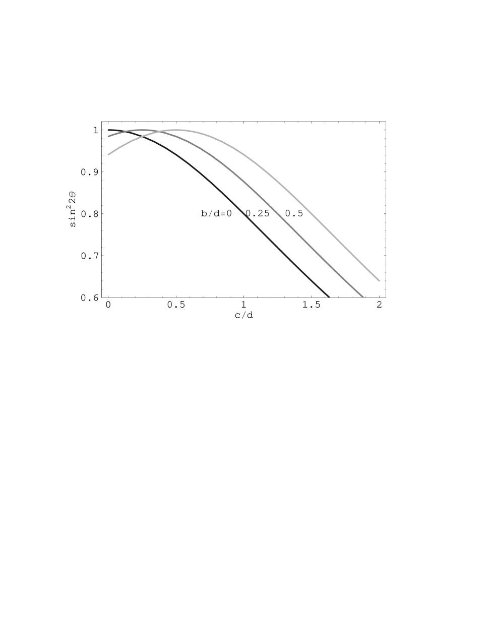
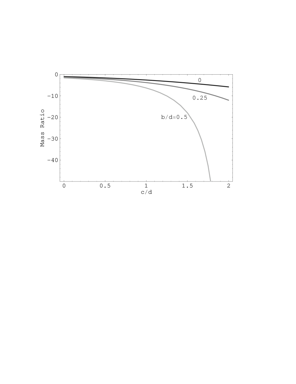
As we see from these figures, the mixing angle can be sufficiently large: $\sin^{2}2\theta_{23}\geq 0.8$ for a significant range of values for $b$ and $c$. In particular, if the diagonal entries are of the same order of magnitude as the off-diagonal ones, large mixing, which may even be amplified by the renormalisation effects discussed below, is generated. Moreover, we observe that such large mixing does not require near-degenerate neutrinos, but is also compatible with larger neutrino mass hierarchies. If either $b$ or $c$ remain close to zero, then the masses tend to be of comparable magnitude. However, if both coefficients start becoming as large as the off-diagonal entries, the mass eigenvalues may spread out, while the mixing angle may remain large. Cancellations can arise automatically in the calculation of the lighter mass eigenvalue, as we subtract entries of comparable magnitudes. To illustrate this, let us look at a specific set of values: for $b=0.5,\;c=1.5$ and $d=1$, sin${}^{2}2\theta_{23}=0.8$. However, the eigenvalues are 2.1 and -0.1, differing by a factor of 20.

We conclude that the hierarchy $m_{3}\approx 10^{-1}$ to $10^{-1.5}$ eV $>>m_{2}\approx 10^{-2.5}$ eV $>>m_{1}$ is compatible with a large mixing angle $\sin^{2}2\theta_{23}\geq 0.8$ as suggested by the atmospheric and solar neutrino data. On the other hand, obtaining the 1% or better degeneracy between $m_{2}$ and $m_{3}$ that would be required in option (c) above, where there is significant hot dark matter, would require a tighter adjustment of parameters that appears less natural, if there is no corresponding symmetry.

III-B. Possible Textures of Dirac and Majorana Mass Matrices

Having commented on the possible structure of $m_{eff}$, the next question is: from what forms of Dirac and heavy Majorana mass structures may we obtain the desired $m_{eff}$? The form of the heavy Majorana mass matrix $M_{\nu_{R}}$ may easily be found from (10), once the neutrino Dirac mass matrix has been specified. It is clear that if the neutrino Dirac mass matrix is diagonal, one particular solution is

$$M_{\nu_{R}}\propto(M_{\nu_{R}})^{-1}\propto m_{eff}\propto\left(\begin{array}[]{cc}0&1\\ 1&0\end{array}\right)$$ (17)

Of course, as the Dirac mass matrix changes, different forms of $M_{\nu_{R}}$ are required in order to obtain the required form of $m_{eff}$. This is exemplified in Table 1, where we show the textures that lead to $m_{eff}$ as given in (17) for various forms of symmetric Dirac mass matrices. In the case of asymmetric mass matrices, one would have more freedom in the choice of the expansion parameters , as seen in Table 2. There we repeat the analysis of Table 1 for the extreme case that one off-diagonal entry of the $2\times 2$ mass matrix is set to zero.

$m_{\nu}^{D}$	$(m_{\nu}^{D})^{Diag}$	$M_{\nu_{R}}$	$M_{\nu_{R}}^{Diag}$
$\left(\begin{array}[]{cc}\lambda&\lambda^{2}\\ \lambda^{2}&1\end{array}\right)$	$\left(\begin{array}[]{cc}\lambda&0\\ 0&1\end{array}\right)$	$M_{N}\left(\begin{array}[]{ccc}2\lambda^{2}&1\\ 1&2\lambda\end{array}\right)$	$M_{N}\left(\begin{array}[]{cc}-1&0\\ 0&1\end{array}\right)$
$\left(\begin{array}[]{cc}\lambda^{2}&\lambda^{2}\\ \lambda^{2}&1\end{array}\right)$	$\left(\begin{array}[]{cc}\lambda^{2}&0\\ 0&1\end{array}\right)$	$M_{N}\left(\begin{array}[]{ccc}2\lambda^{2}&1\\ 1&2\end{array}\right)$	$M_{N}\left(\begin{array}[]{cc}(1-\sqrt{2})&0\\ 0&(1+\sqrt{2})\end{array}\right)$
$\left(\begin{array}[]{cc}\lambda^{3}&\lambda^{2}\\ \lambda^{2}&1\end{array}\right)$	$\left(\begin{array}[]{cc}\lambda^{3}&0\\ 0&1\end{array}\right)$	$M_{N}\left(\begin{array}[]{ccc}2\lambda^{3}&\lambda\\ \lambda&2\end{array}\right)$	$M_{N}\left(\begin{array}[]{ccc}-\lambda^{2}/2&0\\ 0&2\end{array}\right)$
$\left(\begin{array}[]{cc}\lambda&1\\ 1&\lambda\end{array}\right)$	$\left(\begin{array}[]{cc}-1&0\\ 0&1\end{array}\right)$	$M_{N}\left(\begin{array}[]{ccc}2\lambda&1\\ 1&2\lambda\end{array}\right)$	$M_{N}\left(\begin{array}[]{ccc}-1&0\\ 0&1\end{array}\right)$
$\left(\begin{array}[]{cc}\lambda^{2}&1\\ 1&\lambda\end{array}\right)$	$\left(\begin{array}[]{cc}-1&0\\ 0&1\end{array}\right)$	$M_{N}\left(\begin{array}[]{cc}2\lambda^{2}&1\\ 1&2\lambda\end{array}\right)$	$M_{N}\left(\begin{array}[]{cc}-1&0\\ 0&1\end{array}\right)$

Table 1: Approximate forms for some of the basic structures of symmetric textures, keeping the dominant contributions.

$m_{\nu}^{D}$	$(m_{\nu}^{D})^{Diag}$	$M_{\nu_{R}}$	$M_{\nu_{R}}^{Diag}$
$\left(\begin{array}[]{cc}\lambda&0\\ \lambda^{2}&1\end{array}\right)$	$\left(\begin{array}[]{cc}\lambda&0\\ 0&1\end{array}\right)$	$M_{N}\left(\begin{array}[]{ccc}2\lambda^{2}&1\\ 1&0\end{array}\right)$	$M_{N}\left(\begin{array}[]{cc}-1&0\\ 0&1\end{array}\right)$
$\left(\begin{array}[]{cc}\lambda^{2}&0\\ \lambda^{2}&1\end{array}\right)$	$\left(\begin{array}[]{cc}\lambda^{2}&0\\ 0&1\end{array}\right)$	$M_{N}\left(\begin{array}[]{ccc}2\lambda^{2}&1\\ 1&0\end{array}\right)$	$M_{N}\left(\begin{array}[]{cc}-1&0\\ 0&1\end{array}\right)$
$\left(\begin{array}[]{cc}\lambda^{3}&0\\ \lambda^{2}&1\end{array}\right)$	$\left(\begin{array}[]{cc}\lambda^{3}&0\\ 0&1\end{array}\right)$	$M_{N}\left(\begin{array}[]{ccc}2\lambda^{2}&1\\ 1&0\end{array}\right)$	$M_{N}\left(\begin{array}[]{ccc}-1&0\\ 0&1\end{array}\right)$
$\left(\begin{array}[]{cc}\lambda&0\\ 1&\lambda\end{array}\right)$	$\left(\begin{array}[]{cc}\lambda^{2}&0\\ 0&1\end{array}\right)$	$M_{N}\left(\begin{array}[]{ccc}2&\lambda\\ \lambda&0\end{array}\right)$	$M_{N}\left(\begin{array}[]{ccc}2&0\\ 0&-\lambda^{2}/2\end{array}\right)$
$\left(\begin{array}[]{cc}\lambda^{2}&0\\ 1&\lambda\end{array}\right)$	$\left(\begin{array}[]{cc}\lambda^{3}&0\\ 0&1\end{array}\right)$	$M_{N}\left(\begin{array}[]{cc}2&\lambda\\ \lambda&0\end{array}\right)$	$M_{N}\left(\begin{array}[]{cc}2&0\\ 0&-\lambda^{2}/2\end{array}\right)$

Table 2: Approximate forms for some of the basic structures of asymmetric textures, keeping the dominant contributions.

Let us now make a few comments on the tables, looking first at the case of symmetric Dirac mass matrices. For the first texture, the Dirac mass matrix is almost diagonal, so a large mixing in the heavy Majorana sector is directly communicated to $m_{eff}$. In the third example, however, we see that a large mixing angle in the heavy Majorana sector may not lead to a large mixing in $m_{eff}$. In this case, in order to obtain a large mixing in $m_{eff}$, we require a totally different heavy Majorana mass texture, with the larger element in the diagonal. Let us now look at the third example of the second table. This texture is similar to the one we just discussed, with the exception of a zero in the (1,2) position. The appearance of this zero brings us back to the case where the large mixing in the heavy Majorana sector is communicated to $m_{eff}$. These observations, although simple, are of interest when we come to consider specific examples in the framework of flavour symmetries in realistic models at a later point in our discussion.

III-C. Mixing-Angle Relations

Equipped with these illustrative examples, we now discuss in a more general way how the mixing angles and mass hierarchies in the various sectors are related, in particular by relaxing the specific form (17) of $M_{\nu_{R}}$. We consider the case of a symmetric Dirac mass matrix with mixing angle $\vartheta$, define $\phi$ to be the mixing angle in the heavy Majorana neutrino mass matrix, and denote by $\theta$ the resulting mixing angle in the light-neutrino mass matrix $m_{eff}$ . The heavy Majorana mass matrix can be parametrised as

$$M_{\nu_{R}}=\left(\begin{array}[]{cc}M_{2}\cos^{2}\phi+M_{3}\sin^{2}\phi&(M_{2}-M_{3})\cos\phi\sin\phi\\ (M_{2}-M_{3})\cos\phi\sin\phi&M_{3}\cos^{2}\phi+M_{2}\sin^{2}\phi\end{array}\right)$$ (20)

where the mixing angle is given by

$$\tan 2\phi=\frac{\sin(4\vartheta-2\theta)+r^{2}\sin 2\theta-2rR\sin 2\vartheta}{\cos(4\vartheta-2\theta)+r^{2}\cos 2\theta-2rR\cos 2\vartheta}$$ (21)

Here, $M_{3}$ and $M_{2}$ are the eigenvalues of the heavy Majorana mass matrix , $R\equiv(m_{2}+m_{3})/(m_{3}-m_{2})$ where $m_{i}$ are the eigenvalues of the light-neutrino mass matrix, and $r\equiv(m^{D}_{2}+m^{D}_{3})/(m^{D}_{3}-m^{D}_{2})$, where the $m^{D}_{i}$ are the eigenvalues of the Dirac mass matrix. In the limit where $m_{2}=m_{3}$ (note that the signs have to be the same) we have $\tan 2\phi=\tan 2\vartheta$, while in the limit $m_{2}^{D}=m_{3}^{D}$, $\tan 2\phi=\tan 2\theta$. Motivated by the equivalence at the unification scale of the $u$-quark and neutrino Dirac mass matrices in several GUTs, in Fig. 3 we plot $\sin^{2}2\phi$ as a function of $\vartheta$ for $\theta=\pi/4$ and $r=(180+1.4)/(180-1.4)\approx(m_{t}+m_{c})/(m_{t}-m_{c})\approx 1.01$, for three values of $R$: 0, 1 and 10. Fig. 4 shows the same plots, but for $r=3$.

Figure 3: The $2\times 2$ heavy Majorana mixing angle as a function of the mixing angle $\vartheta$ in $m_{\nu}^{D}$, assuming a large hierarchy in its eigenvalues $r\equiv(m^{D}_{2}+m^{D}_{3})/(m^{D}_{3}-m^{D}_{2})$, for selected values of $R\equiv(m_{2}+m_{3})/(m_{3}-m_{2})$.

Figure 4: As for Fig.3, assuming instead a small hierarchy of eigenvalues in $m_{\nu}^{D}$.

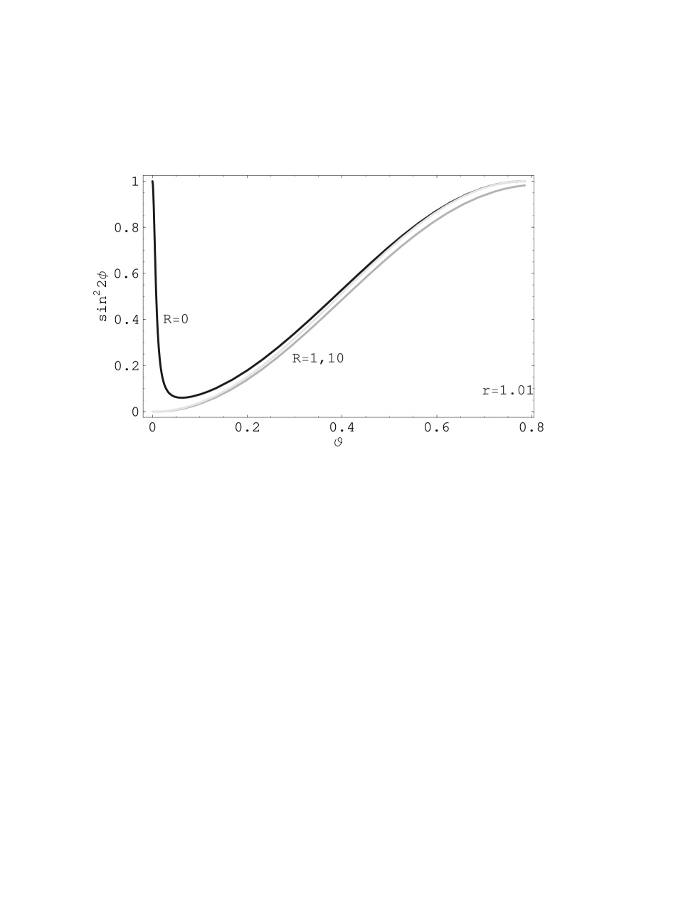
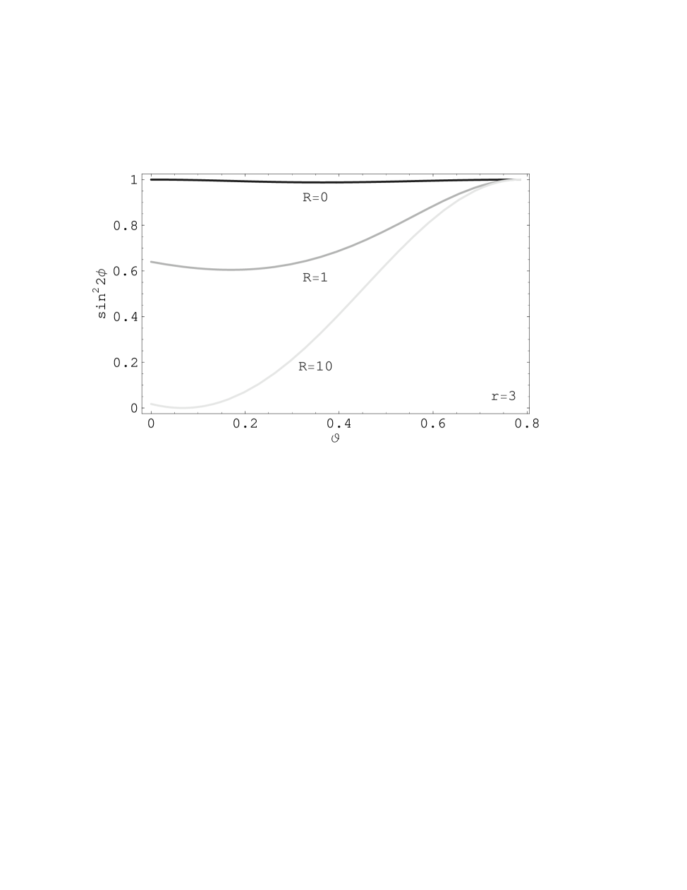
The parameters chosen for the plots are representative of examples with small and large hierarchies in $m_{eff}$ and $m_{\nu}^{D}$: the choice $R=0$ describes the case with $m_{2}=-m_{3}$, which we presented in Tables 1 and 2. This structure arises when the off-diagonal entries of $m_{eff}$ are equal in magnitude, whilst being much larger than the diagonal elements. The choice $R=1$ represents examples with large hierarchies (where $m_{2}$ can be neglected), while $R=10$ describes a case with $m_{2}=(9/11)m_{3}$, which is a typical example where $m_{2}$ and $m_{3}$ are close in magnitude but have the same sign. Concerning the Dirac neutrino masses: the case with $r=(180+1.4)/(180-1.4)\approx 1.01$ is typical of what one may expect in many unified (or partially unified) models, where $m_{\nu}^{D}\sim m_{u}^{D}$. The choice $r=3$, on the other hand, corresponds to the case where $m_{2}^{D}=m_{3}^{D}/2$. This is a complementary example, with small hierarchies in $m_{\nu}^{D}$.

In Fig. 3, we study a case with a large hierarchy in the Dirac mass matrix, much as could be expected in a wide number of unified or partially unified models. In this example, $R=0$ corresponds to the case where the two eigenvalues of $m_{eff}$ are equal, but with opposite signs. This describes examples that appear in Table 1. In such a case, maximal mixing in $M_{\nu_{R}}$ ($\sin^{2}2\phi=1)$, is obtained for a diagonal Dirac mass matrix ($\vartheta=0$). This corresponds to the first example of Table 1. For the same value of $R$, as $\vartheta$ starts increasing, a different form of $M_{\nu_{R}}$ with a smaller (2,3) mixing has a similar effect. This is what we see in example 3 of Table 1.

However, in the limit that $\vartheta$ becomes quite large, we again reach a solution with a large mixing in $M_{\nu_{R}}$. This is indicated in the examples 4 and 5 of Table 1, where we see clearly this amplification of the mixing in the heavy Majorana sector, as the off-diagonal entries of the Dirac mass matrix become the dominant ones. Notice also that example 2 indicates that when the off-diagonal elements of the Dirac mass matrix become of the order of the (1,1) element, already the mixing in $M_{\nu_{R}}$ has increased significantly. On the other hand, we note that when the Dirac neutrino mass matrix exhibits only a small hierarchy, this picture is altered and $R=0$ leads generically to a large mixing. Indeed, again from Table 1, we see that for $\lambda\approx O(1)$, the mixing in the heavy Majorana mass matrix is always large.

In the limit when $R\rightarrow 1$, $|m_{2}|\ll|m_{3}|$. Fig. 3 shows that, in this case, maximal mixing in the light-neutrino sector can be obtained with negligible mixing in the heavy Majorana sector. Thus, for large hierarchies, even with a diagonal Dirac matrix, we can get a large angle in $m_{eff}$ even for small mixing in the heavy Majorana. This result might at first seem rather surprising, but is related to the fact that the solutions to the light-eigenvalue problem are quite sensitive. It is also worth remembering that, if $m_{eff}^{11}\approx m_{eff}^{22}$, then the mixing angle is large, even if the off-diagonal entries of $m_{eff}$ are very small. Let us work out formulae (18,19) in this limiting case. We denote by $m_{2,3}$ the light neutrino eigenmasses and assume maximal mixing. In this case, the form of $m_{eff}$ is given by

$$m_{eff}=\left(\begin{array}[]{cc}m_{2}+m_{3}&m_{2}-m_{3}\\ m_{2}-m_{3}&m_{3}+m_{2}\end{array}\right)$$ (24)

and its inverse by

$$m_{eff}^{-1}=\frac{1}{4m_{2}m_{3}}\left(\begin{array}[]{cc}m_{2}+m_{3}&m_{3}-m_{2}\\ m_{3}-m_{2}&m_{2}+m_{3}\end{array}\right)$$ (27)

If $m_{c},m_{t}$ (equal to the quark masses at the unification scale) are the entries in the diagonal Dirac mass matrix, then the heavy Majorana mass matrix that leads to maximal mixing is given by

$$M_{\nu_{R}}\sim\left(\begin{array}[]{cc}(m_{2}+m_{3})m_{c}^{2}&(m_{3}-m_{2})m_{c}m_{t}\\ (m_{3}-m_{2})m_{c}m_{t}&(m_{3}+m_{2})m_{t}^{2}\end{array}\right)$$ (30)

with a mixing $\tan 2\phi=2(m_{2}+m_{3})m_{c}^{2}/((m_{3}-m_{2})(m_{t}^{2}-m_{c}^{2}))$. For $m_{3}\gg m_{2}$ this mixing is indeed small if the Dirac mass hierarchies are large: $\tan 2\phi\sim m_{c}/m_{t}$. However, if the Dirac mass hierarchies are smaller, then the mixing angle increases in this case as well. This we can see in more detail in Fig. 4.

Let us now comment on the sensitivity of this solution. Suppose we keep $M_{\nu_{R}}$ as above, but modify the second eigenvalue of the Dirac mass matrix to $km_{t}$. In this case, the mixing angle of $m_{eff}$ is found to be

$$\sin^{2}2\theta=\frac{4k^{2}}{(1+k^{2})^{2}}$$ (31)

For $k=1$, we find sin${}^{2}2\theta=1$, which falls to sin${}^{2}2\theta=0.8$ for $k\approx 0.6$. Continuing to $k=1/2$, we find sin${}^{2}2\theta=0.64$, and for $k=1/4$ we obtain sin${}^{2}2\theta=0.22$. We conclude that sin${}^{2}2\theta$ is in the preferred region $\geq 0.8$ for quite a generic range of values of $k$.

To conclude this Section, we note that the case $R=10$ is also shown in the Figs. 3, 4. We see that it is similar to the previous one, but with smaller sin${}^{2}2\phi$ than in the other cases, in the case of a small Dirac mass hierarchy.

This phenomenological analysis indicates that solutions to the atmospheric neutrino problem correlate and severely constrain the masses and mixing hierarchies in the Dirac and heavy Majorana sectors. We note that large mixing is not necessarily incompatible with a large hierarchy between two neutrino masses. The outcome of this discussion can serve as a guideline in constructing realistic models of neutrino masses, as we do in section 7. Before that, however, we analyze possible modifications of the above results due to renormalization-group effects, and then we discuss how this $2\times 2$ analysis may be embedded in a fuller $3\times 3$ analysis.

4. Renormalization-Group Effects

Up to now, we have discussed the situation in which a maximal (23) mixing angle appears already at the GUT scale. However, this is not the only possibility. Within the minimal supersymmetric extension of the Standard Model (MSSM), it has been found that renormalisation group effects may amplify the mixing [19, 20]. Whether this happens depends on the magnitude of $h_{\tau}$: for large $h_{\tau}$, for which large large tan$\beta$ is necessary, the (23) and (13) mixing angles may be amplified significantly. For some examples, initial values of sin$\theta_{23}\geq 0.3$ can lead to large mixing at low energies [21, 22], and similar results have been found for the (13) mixing at large tan$\beta$. On the other hand, the (12) mixing remains essentially unchanged even for large tan$\beta$, and renormalisation-group effects can be neglected for small tan$\beta$. We now discuss such renormalization-group effects in more detail.

IV-A. Renormalization-Group Equations

Between the GUT scale and the scale of the heavy Majorana neutrinos, $M_{N}$, there is an effect on the mixing angle due to the running  of the Dirac neutrino coupling $Y_{N}$:

$$8\pi^{2}{d\over dt}({Y}_{N}{Y}_{N}^{\dagger}) = \{-\sum_{i}c_{N}^{i}g_{i}^{2}+3({Y}_{N}{Y}_{N}^{\dagger})+{\rm Tr}[3({Y}_{U}{Y}_{U}^{\dagger})+({Y}_{N}{Y}_{N}^{\dagger})]\}({Y}_{N}{Y}_{N}^{\dagger})$$ (32)

$$\qquad\qquad+{1\over 2}\{({Y}_{E}{Y}_{E}^{\dagger})({Y}_{N}{Y}_{N}^{\dagger})+({Y}_{N}{Y}_{N}^{\dagger})({Y}_{E}{Y}_{E}^{\dagger})\}$$

where $t$ is the logarithmic renormalization-group scale, $c^{i}_{N}=(3/5,3,0)$ for the MSSM, and we denote the Dirac couplings of other types of fermion $F$ by $Y_{F}$. We see from these equations that the various entries of $m^{D}$ run differently: large Yukawa couplings, which lower $Y_{N}$, have a bigger effect on $m^{D}_{33}$ than on the rest of the elements. This alters the structure of the Dirac mass matrix, in turn affecting the magnitude of the mixing angle. The effect becomes more relevant in examples where cancellations between various entries may lead to amplified mixing in $m_{eff}$.

Below the right-handed Majorana mass scale, ${Y}_{N}$ decouples and the relevant running is that of the effective neutrino mass operator [20]:

$$8\pi^{2}{d\over dt}{m_{eff}}=\{-({3\over 5}g_{1}^{2}+3g_{2}^{2})+{\rm Tr}[3{Y}_{U}{Y}_{U}^{\dagger}]\}m_{eff}+{1\over 2}\{({Y}_{E}{Y}_{E}^{\dagger})m_{eff}+m_{eff}({Y}_{E}{Y}_{E}^{\dagger})^{T}\}\ ,$$ (33)

which we use later to study the variation in the diagonal entries in $m_{eff}$. Off-diagonal entries enter into the neutrino mixing angle $\theta_{23}$, whose running is given by [20]:

$$16\pi^{2}{d\over dt}{\sin^{2}2\theta_{23}}=-2\sin^{2}2\theta_{23}(1-\sin^{2}2\theta_{23})(Y_{E3}^{2}-Y_{E2}^{2}){m_{eff}^{33}+m_{eff}^{22}\over m_{eff}^{33}-m_{eff}^{22}}\$$ (34)

As this equation indicates, sin${}^{2}2\theta_{23}$ may be particularly strongly affected as one runs down from the GUT to the electroweak scale (i) if $Y_{E3}$ is large, and (ii) if the diagonal entries of $m_{eff}$ are close in magnitude. Thus the exact evolution of the mixing angle depends on the particular texture being studied.

In general, the amplification effects that one may obtain for large tan$\beta$ are of the order of 30 - 50%, for cases where one starts with a small or moderate value of the mixing angle at the GUT scale. However, in particular combinations of textures for the Dirac and the heavy Majorana mass matrices, cancellations between various terms may lead to even larger amplifications of the mixing angles. It has been noted in such cases that the running of the Yukawa couplings between the GUT scale and the effective $M_{N}$ scale may strengthen such cancellation effects, thus increasing the mixing significantly [21]. A similar effect may arise below $M_{N}$. Examination of the equation (34) that describes the running of the mixing angle indicates that significant amplification may be obtained for textures where $m_{eff}^{22}$ and $m_{eff}^{33}$ are close in magnitude [20].

IV-B. Semi-Analytic Solutions

In order to get a better feeling for the magnitude of the mixing angle, it is useful to look for semi-analytic solutions to one-loop equations (33,34). To do so, we start with the differential equations for the diagonal elements of the effective neutrino mass matrix. These are given by

$$\frac{1}{m_{eff}^{22}}\frac{d}{dt}m_{eff}^{22} = \frac{1}{8\pi^{2}}\left(-c_{i}g_{i}^{2}+3h_{t}^{2}\right)$$ (35)

$$\frac{1}{m_{eff}^{33}}\frac{d}{dt}m_{eff}^{33} = \frac{1}{8\pi^{2}}\left(-c_{i}g_{i}^{2}+3h_{t}^{2}+h_{\tau}^{2}\right)$$ (36)

For the $m_{eff}^{33}$ element, simple integration yields

$$\frac{m_{eff}^{33}}{m_{eff,0}^{33}} = exp\left\{\frac{1}{8\pi^{2}}\int_{t_{0}}^{t}\left(-c_{i}g_{i}^{2}+3h_{t}^{2}+h_{\tau}^{2}\right)\right\}$$ (37)

$$= I_{g}\cdot I_{t}\cdot I_{\tau}$$

where

$$I_{g} = exp[\frac{1}{8\pi^{2}}\int_{t_{0}}^{t}(-c_{i}g_{i}^{2}dt)]$$ (38)

$$I_{t} = exp[\frac{1}{8\pi^{2}}\int_{t_{0}}^{t}h_{t}^{2}dt]$$ (39)

$$I_{\tau} = exp[\frac{1}{8\pi^{2}}\int_{t_{0}}^{t}h_{\tau}^{2}dt]$$ (40)

and $m_{eff,0}^{33}$ is the initial condition. This condition is defined at $M_{N}$, at the stage when $h_{N}$ decouples from the renormalisation-group equations. For simplicity of presentation, we assume for the sake of the following discussion that $M_{N}\approx M_{GUT}$. Similarly, we find that:

$$m_{eff}^{22} = m_{eff,0}^{22}\cdot I_{g}\cdot I_{t}$$ (41)

so that $m_{eff}^{33}/m_{eff}^{22}=I_{\tau}\cdot m_{eff,0}^{33}/m_{eff,0}^{22}$, leading to the formula

$$\frac{m_{eff}^{33}+m_{eff}^{22}}{m_{eff}^{33}-m_{eff}^{22}} = \frac{m_{eff,0}^{33}I_{\tau}+m_{eff,0}^{22}}{m_{eff,0}^{33}I_{\tau}-m_{eff,0}^{22}}\equiv f(I_{\tau})$$ (43)

for the diagonal mass-matrix elements.

We can then convert the one-loop evolution equation (34) for sin${}^{2}\theta$ to a differential equation for $T=\tan^{2}2\theta$:

$$\frac{dT}{T} = -\frac{2}{16\pi^{2}}h_{\tau}^{2}f(I_{\tau})$$ (44)

The solution to (44) is

$$\tan^{2}2\theta = \tan^{2}2\theta_{0}I_{2}(h_{\tau})$$ (45)

with

$$I_{2}(h_{\tau})=exp\left\{-\frac{1}{8\pi^{2}}\int_{t_{0}}^{t}h_{\tau}^{2}f(I_{\tau})\right\}$$ (46)

We see that the only parameters which enter into the final formula are the initial conditions and an integral that incorporates all the renormalization-group running of $h_{\tau}$.

IV-C. Some Implications

The following are the most important deductions we extract from the above equations. Suppose we start with a generic $m_{eff}$ at a high scale: then, $m_{eff}^{33}$ decreases more rapidly than $m_{eff}^{22}$, due to the effect of the $\tau$ Yukawa coupling. If one starts with $m_{eff}^{22}$ and $m_{eff}^{33}$ relatively close in magnitude, the expectation is that at a given scale they may become equal, in which case the mixing angle is maximal. How fast this happens, depends on the magnitude of $h_{\tau}$. The larger $h_{\tau}$, the earlier the entries may become equal. Of course, $h_{\tau}$ also decreases while running down to low energies, and this has also to be taken into account. The scale where the mixing angle is maximal is given by the relation

$$I_{\tau}=\frac{m_{eff,0}^{22}}{m_{eff,0}^{33}}$$ (47)

After reaching the maximal angle at some intermediate scale, the running of $h_{\tau}$ results in

$${m_{eff,0}^{33}}<{m_{eff,0}^{22}}$$

This changes the sign of $f(I_{\tau})$ and results in a rather rapid decrease of the mixing. In order, therefore, for a texture of this type to be viable, there needs to be a balance between the magnitudes of $h_{\tau}$ and $m_{eff}^{33}-m_{eff}^{22}$ at the GUT scale. If the splitting is small and the coupling large, then the maximal value for the mixing will be obtained too early to survive at low energies.

Let us explore the circumstances under which the mixing becomes close to maximal at low scales. We consider an example where $h_{\tau}=h_{t}=h_{b}\equiv h=3$, $M_{GUT}=1.1\times 10^{16}$ GeV and the common gauge coupling at the unification scale is $0.039$. Also, we take the scale of supersymmetry breaking to be around 1 TeV. We find that a texture [20] with

$$m_{eff}^{22}=0.6,\;\;\;m_{eff}^{23}=0.035,\;\;\;m_{eff}^{33}=1.0,$$ (48)

which has a starting value for the mixing given by sin${}^{2}2\theta\approx 0.03$, reaches maximal mixing: sin${}^{2}2\theta\sim 1$ at $\approx 1$ TeV. If we assume the same texture but take $h=2$, the mixing is only sin${}^{2}2\theta\approx 0.35$ at $\approx 1$ TeV. However, for the same coupling, making the modification to $m_{eff}^{22}=0.7$ leads to maximal mixing at around 5.5 TeV. Finally, for $h=1$ at the GUT scale, we need to modify $m_{eff}^{22}$ to approximately 0.8, in order for maximal mixing to occur around the TeV scale.

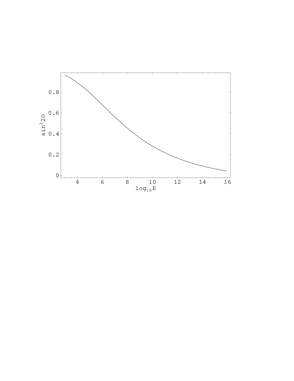
Let us also look at another specific example texture. We assume the texture

$$m_{eff}=\left(\begin{array}[]{cc}1-x&x^{2}\\ x^{2}&1+x\end{array}\right)$$ (49)

with $x\approx 0.2$, so that the off-diagonal elements are much smaller than the mass splitting of the diagonal ones. We are going to see that renormalisation group effects will lead to a very large increase of the mixing angle. In this case, the one-loop running of the mixing angle is indicated in Fig. 5. Here we took as initial conditions: $M_{N}\approx M_{GUT}=10^{16}$ GeV, a common coupling at the unification scale $0.042$ and $h_{t}=h_{b}=h_{\tau}=2.0$. This running indicates that, for this example, the mixing has indeed changed significantly as we run down to lower energies.

Figure 5: An example of the renormalisation-group enhancement of the $2\times 2$ light-neutrino mixing angle, starting from a small value at the GUT scale. We assume initial Yukawa couplings $h_{t}=h_{b}=h_{\tau}=2.0$, corresponding to a large value of $tan\beta$.

5. Sample Textures in Three-Generation Examples

So far, we have worked in the limit where the solar neutrino problem is resolved by a small mixing angle. However, this need not be the case, and one should consider what happens if this mixing is also large . In this case, we need to consider the general $3\times 3$ mixing problem. We can clearly proceed as in the case of 2 $\times 2$ mixing, and investigate the relations between the mixing angles and hierarchies in the Dirac, heavy and light Majorana mass matrices. However, the number of parameters is very large, and one cannot proceed far without making assumptions on the patterns of mixing and the structure of the mass matrices. We write the generic form of a $3\times 3$ mixing-angle matrix (ignoring phases) in the form

$$V_{3\times 3}=\left(\begin{array}[]{ccc}c_{12}&-s_{12}c_{13}&-s_{12}s_{13}\\ s_{12}c_{23}&c_{12}c_{23}c_{13}+s_{23}s_{13}&c_{12}c_{23}s_{13}-s_{23}c_{13}\\ s_{12}s_{23}&c_{12}s_{23}c_{13}-c_{23}s_{13}&c_{12}s_{23}s_{13}+c_{23}c_{13}\end{array}\right)$$ (50)

where $s_{ij},c_{ij}$ stand for $\sin\theta_{ij}$ and $\cos\theta_{ij}$, respectively, and will explore the implications of various possible hierarchies between the angles $\theta_{ij}$. Investigating the possible hierarchies within $m_{eff}$ is then straightforward.

V-A. Cases with Maximal Mixing

We first assume for simplicity of discussion that $\theta_{23}$ is maximal , and that $\theta_{12}\gg\theta_{13}\sim 0$. In this case, $m_{eff}=V_{3\times 3}.m_{eff}^{diag}.V_{3\times 3}^{\dagger}$ is given by

$$m_{eff}=\left(\begin{array}[]{ccc}m_{1}c_{12}^{2}+m_{2}s_{12}^{2}&\frac{(m_{1}-m_{2})c_{12}s_{12}}{\sqrt{2}}&\frac{(m_{1}-m_{2})c_{12}s_{12}}{\sqrt{2}}\\ \frac{(m_{1}-m_{2})c_{12}s_{12}}{\sqrt{2}}&\frac{1}{2}(m_{3}+m_{1}s_{12}^{2}+m_{2}c_{12}^{2})&\frac{1}{2}(-m_{3}+m_{1}s_{12}^{2}+m_{2}c_{12}^{2})\\ \frac{(m_{1}-m_{2})c_{12}s_{12}}{\sqrt{2}}&\frac{1}{2}(-m_{3}+m_{1}s_{12}^{2}+m_{2}c_{12}^{2})&\frac{1}{2}(m_{3}+m_{1}s_{12}^{2}+m_{2}c_{12}^{2})\end{array}\right)$$ (51)

and one may look at the implications for mass hierarchies. Initially, we prefer to simplify further to the case of maximal $\theta_{12},\theta_{23}$ mixing. In this case,

$$m_{eff}=\left(\begin{array}[]{ccc}\frac{m_{1}+m_{2}}{2}&\frac{m_{1}-m_{2}}{2\sqrt{2}}&\frac{m_{1}-m_{2}}{2\sqrt{2}}\\ \frac{m_{1}-m_{2}}{2\sqrt{2}}&\frac{1}{4}(m_{1}+m_{2}+2m_{3})&\frac{1}{4}(m_{1}+m_{2}-2m_{3})\\ \frac{m_{1}-m_{2}}{2\sqrt{2}}&\frac{1}{4}(m_{1}+m_{2}-2m_{3})&\frac{1}{4}(m_{1}+m_{2}+2m_{3})\end{array}\right)$$ (52)

We saw in Section 3 that, when all the entries of a $2\times 2$ matrix are of the same order of magnitude, plausible cancellations may still lead to large hierarchies between the eigenvalues, even in the presence of a large mixing. We can visualize the type of texture of $3\times 3$ $m_{eff}$ (52) that is consistent with such maximal mixing by considering specific limiting cases for the $m_{i}$.

For example, in the limit $m_{3}\gg m_{2}\gg m_{1}$, one has

$$m_{eff}={m_{3}\over 2}\left(\begin{array}[]{ccc}0&0&0\\ 0&1&-1\\ 0&-1&1\end{array}\right)+{m_{2}\over 2}\left(\begin{array}[]{ccc}1&-{1\over\sqrt{2}}&-{1\over\sqrt{2}}\\ -{1\over\sqrt{2}}&{1\over 2}&{1\over 2}\\ -{1\over\sqrt{2}}&{1\over 2}&{1\over 2}\end{array}\right)+{m_{1}\over 2}\left(\begin{array}[]{ccc}1&{1\over\sqrt{2}}&{1\over\sqrt{2}}\\ {1\over\sqrt{2}}&{1\over 2}&{1\over 2}\\ {1\over\sqrt{2}}&{1\over 2}&{1\over 2}\end{array}\right)$$ (53)

On the other hand, if one considers near-degenerate cases $m\equiv m_{3}\sim m_{2}\sim m_{1}:\Delta\equiv|m_{3}|-|m_{2}|\gg\delta\equiv|m_{2}|-|m_{1}|$, there are various possibilities, distinguished by the relative signs of the eigenvalues. For example, if all the eigenvalues have the same sign, one finds the texture:

$$m_{eff}=m_{2}\left(\begin{array}[]{ccc}1&0&0\\ 0&1&0\\ 0&0&1\end{array}\right)+\frac{\Delta}{2}\left(\begin{array}[]{ccc}0&0&0\\ 0&1&-1\\ 0&-1&1\end{array}\right)-\frac{\delta}{2}\left(\begin{array}[]{ccc}1&{1\over\sqrt{2}}&{1\over\sqrt{2}}\\ {1\over\sqrt{2}}&{1\over 2}&{1\over 2}\\ {1\over\sqrt{2}}&{1\over 2}&{1\over 2}\end{array}\right)$$ (54)

On the other hand, if one of the eigenvalues has a different sign from the other two, this structures get modified. Suppose, for example, that $m_{1}$ and $m_{3}$ are positive and $m_{2}$ negative. We the find

$$m_{eff}=\frac{m_{2}}{2}\left(\begin{array}[]{ccc}0&{-2\over\sqrt{2}}&{-2\over\sqrt{2}}\\ {-2\over\sqrt{2}}&-1&1\\ {-2\over\sqrt{2}}&1&-1\end{array}\right)+\frac{\Delta}{2}\left(\begin{array}[]{ccc}0&0&0\\ 0&1&-1\\ 0&-1&1\end{array}\right)-\frac{\delta}{2}\left(\begin{array}[]{ccc}1&{1\over\sqrt{2}}&{1\over\sqrt{2}}\\ {1\over\sqrt{2}}&{1\over 2}&{1\over 2}\\ {1\over\sqrt{2}}&{1\over 2}&{1\over 2}\end{array}\right)$$ (55)

We return later to these suggestive examples, but first discuss how $m_{eff}$ may be derived from the primary Dirac and Majorana mass matrices of the fundamental theory, which may be some GUT and/or string model.

V-B. Heavy Majorana Mass Textures with Matched Mixing

Up to now, we have been discussing possible forms of $m_{eff}$ that are consistent with the atmospheric and solar neutrino data. However, in a more fundamental model, the gauge group structure, as well as possible $U(1)$ symmetries and string selection rules, predict the structure of the Dirac and heavy Majorana matrices, while $m_{eff}$ is a secondary output of the see-saw mechanism. Thus, to make contact with such unified (or partially unified) theories, it is essential to analyze the forms of Dirac and heavy Majorana mass matrices that are suggested by the experimental data. Such an analysis may reveal relations between the mass and mixing hierarchies of the different neutrino sectors that can then be used as a guideline in investigations that involve realistic models, as we discuss in Section 7.

In general, calculating the heavy Majorana mass matrix involves 12 parameters: the 6 eigenvalues of $m_{\nu}^{D}$ and $m_{eff}$ and 3 mixing angles for each of these two matrices. General formulae for all the entries in the full $3\times 3$ $M_{\nu_{R}}$ matrix in terms of all these parameters are easily derived but quite complicated, and are not given here. Instead, we look at some limiting cases. It is convenient to parametrize these cases in terms of the hierarchy factors $x\equiv m_{1}/m_{3},y\equiv m_{2}/m_{3}$ for the ratios of eigenvalues of $m_{eff}$ and $\lambda_{1}\equiv M_{\nu_{R},1}/M_{\nu_{R},3},\lambda_{2}\equiv M_{\nu_{2}}^{D}/M_{\nu_{3}}^{D}$ for the ratios of eigenvalues of the neutrino Dirac mass matrix $m_{\nu}^{D}$.

We initially assume one large mixing angle in the effective light Majorana matrix. Then, we can distinguish two cases for the structure of the heavy Majorana matrix. The first is that of matched mixing, when there is no large mixing in other sectors of either the light Majorana or the Dirac matrices, in which case the problem is equivalent to the $2\times 2$ case considered previously. In particular, consider first the possibility that the Dirac mass matrix is diagonal to a good approximation. Then, the form of the heavy Majorana mass matrix becomes

$$M_{\nu_{R}}\propto\left(\begin{array}[]{ccc}\lambda_{1}^{2}\over x&0&0\\ 0&\lambda_{2}^{2}(y+1)\over 2y&\lambda_{2}(y-1)\over 2y\\ 0&\lambda_{2}(y-1)\over 2y&(y+1)\over 2y\end{array}\right)$$ (56)

In the particular case that $y=m_{2}/m_{3}=-1$, this leads to a texture of the form

$$M_{\nu_{R}}\propto\left(\begin{array}[]{ccc}\lambda_{1}^{2}\over x&0&0\\ 0&0&\lambda_{2}\\ 0&\lambda_{2}&0\end{array}\right)$$ (57)

which resembles one of the popular $2\times 2$ textures in Table 1.

Alternatively, for large hierarchies in $m_{eff}$, i.e., for small mass ratios; $x\ll y\ll 1$, the form of the heavy Majorana mass matrix becomes

$$M_{\nu_{R}}\propto\left(\begin{array}[]{ccc}\lambda_{1}^{2}\over x&0&0\\ 0&\lambda_{2}^{2}\over 2y&\lambda_{2}\over 2y\\ 0&\lambda_{2}\over 2y&1\over 2y\end{array}\right)$$ (58)

which has some similarities with textures displayed in Table 1, but is not identical. This texture shows that, for large hierarchies in $m_{eff}$ and an almost diagonal $M_{\nu}^{D}$, the (23) mixing in $M_{\nu_{R}}$ scales as $\lambda_{2}$. This is consistent with what we found in Figs. 3 and 4. we recall that large hierarchies in $m_{eff}$ are described by the limit $R\rightarrow 1$. We see in Fig. 4 that, for small Dirac hierarchies and negligible Dirac mixing angle $\vartheta$, the angle $\phi$ that describes (23) mixing in $M_{\nu_{R}}$ has intermediate values. However, as the Dirac hierarchies become large, $\phi$ becomes very small, as is indicated in Fig. 3.

If, however, we take the Dirac mass matrix to have maximal (23) mixing, the general texture (56) becomes

$$M_{\nu_{R}}\propto\left(\begin{array}[]{ccc}\lambda_{1}^{2}\over x&0&0\\ 0&(\lambda_{2}^{2}+y)\over 2y&(-\lambda_{2}^{2}+y)\over 2y\\ 0&(-\lambda_{2}^{2}+y)\over 2y&(\lambda_{2}^{2}+y)\over 2y\end{array}\right)$$ (59)

and clearly its form depends on the relative magnitudes of $\lambda_{i},x$ and $y$. In the specific case where the $m_{eff}$ hierarchy is much greater than the neutrino Dirac hierarchy: $\lambda_{2}\gg y$, we obtain the texture

$$M_{\nu_{R}}\propto{\rm Diag}{\left({\lambda_{1}^{2}\over x},{\lambda_{2}^{2}\over 2y}{\left(\begin{array}[]{cc}1&-1\\ -1&1\\ \end{array}\right)}\right)}$$ (60)

whereas when the $m_{eff}$ hierarchy is smaller: $\lambda_{2}\ll y$ we find

$$M_{\nu_{R}}\propto{\rm Diag}{\left({\lambda_{1}^{2}\over x},{1\over 2}{\left(\begin{array}[]{cc}1&1\\ 1&1\\ \end{array}\right)}\right)}$$ (61)

We note that (57,60,61) span all but one of the possibilities for the $2\times 2$ submatrix with indices (2,3).

We can again compare these solutions with the results that we presented in Figs. 3 and 4, in the region where the (23) Dirac mixing angle $\vartheta$ becomes maximal. We see in Figs. 3 and 4 that, independently from the Dirac and the $m_{eff}$ mass hierarchies, as $\vartheta$ increases, so does the required mixing in $M_{\nu_{R}}$. Moreover, for small mass differences in $m_{eff}$, the solution corresponds to the last two examples of Table 1, which indicate exactly this effect.

V-C. Mismatched Mixing

A different structure arises when there is more than one mixing angle in $m_{eff}$, or there is a large Dirac mixing angle that involves different generations from those of the light Majorana matrix. This happens, for example, when the atmospheric problem is solved by $\nu_{\mu}\rightarrow\nu_{\tau}$ oscillations whilst the Dirac mass matrix is related to the quark mass matrix, with Cabibbo mixing between the first and second generations. The structure of the Majorana matrix becomes more complicated for this mismatched mixing.

In the case that $m_{eff}$ has two large angles, the textures are of course more complicated than in the previous subsection. To see this, note that for an almost-diagonal Dirac mass matrix, the wanted form of the heavy Majorana mass matrix for $y=-1$ becomes

$$M_{\nu_{R}}\propto\left(\begin{array}[]{ccc}\lambda_{1}^{2}\over 2x&-\lambda_{1}\lambda_{2}\over 2x&\lambda_{1}\over\sqrt{2}\\ -\lambda_{1}\lambda_{2}\over 2x&\lambda_{2}^{2}\over 2x&\lambda_{2}\over\sqrt{2}\\ \lambda_{1}\over\sqrt{2}&\lambda_{2}\over\sqrt{2}&0\end{array}\right)$$ (62)

and for $y\ll 1$ becomes

$$M_{\nu_{R}}\propto\left(\begin{array}[]{ccc}\lambda_{1}^{2}\over 2x&-\lambda_{1}\lambda_{2}\over 2x&-\lambda_{1}\over 2\sqrt{2}y\\ -\lambda_{1}\lambda_{2}\over 2x&\lambda_{2}^{2}\over 2x&-\lambda_{2}\over 2\sqrt{2}y\\ -\lambda_{1}\over 2\sqrt{2}y&-\lambda_{2}\over 2\sqrt{2}y&1\over 2y\end{array}\right)$$ (63)

In such a case, large Dirac hierarchies (and in particular $\lambda_{1}\ll\lambda_{2}$), effectively decouple the light entry of the heavy Majorana mass matrix from the heavier ones.

This is no longer true, however, if the (12) mixing angle in the Dirac mass matrix becomes $\pi/4$, and we still have two large mixing angle in $m_{eff}$.

In this case

$$M_{\nu_{R}}\propto\left(\begin{array}[]{ccc}2\lambda_{1}^{2}y+\lambda_{2}^{2}x(1+y)\over 4xy&-2\lambda_{1}^{2}y+\lambda_{2}^{2}x(1+y)\over 4xy&\lambda_{2}(-1+y)\over 2\sqrt{2}y\\ -2\lambda_{1}^{2}y+\lambda_{2}^{2}x(1+y)\over 4xy&2\lambda_{1}^{2}y+\lambda_{2}^{2}x(1+y)\over 4xy&\lambda_{2}(-1+y)\over 2\sqrt{2}y\\ \lambda_{2}(-1+y)\over 2\sqrt{2}y&\lambda_{2}(-1+y)\over 2\sqrt{2}y&(1+y)\over 2y\end{array}\right)\newline$$ (67)

which, in the limit of a large $m_{eff}$ hierarchy: $y\ll 1$ and $\lambda_{2}^{2}x\gg\lambda_{1}^{2}y$ gives the texture

$$M_{\nu_{R}}\propto\frac{1}{2y}\times\left(\begin{array}[]{ccc}\lambda_{2}^{2}\over 2&\lambda_{2}^{2}\over 2&-\lambda_{2}\over\sqrt{2}\\ \lambda_{2}^{2}\over 2&\lambda_{2}^{2}\over 2&-\lambda_{2}\over\sqrt{2}\\ -\lambda_{2}\over\sqrt{2}&-\lambda_{2}\over\sqrt{2}&1\end{array}\right)$$ (71)

Alternatively, if both the (12) and (23) Dirac mixing angles are maximal,

$$M_{\nu_{R}}\propto\left(\begin{array}[]{ccc}\frac{1}{4}\left(1+{2\lambda_{1}^{2}\over x}+{\lambda_{2}^{2}\over y}\right)&\frac{1}{4}\left(1-{2\lambda_{1}^{2}\over x}+{\lambda_{2}^{2}\over y}\right)&(-\lambda_{2}^{2}+y)\over 2\sqrt{2}y\\ \frac{1}{4}\left(1-{2\lambda_{1}^{2}\over x}+{\lambda_{2}^{2}\over y}\right)&\frac{1}{4}\left(1+{2\lambda_{1}^{2}\over x}+{\lambda_{2}^{2}\over y}\right)&{(-\lambda_{2}^{2}+y)\over 2\sqrt{2}y}\\ {(-\lambda_{2}^{2}+y)\over 2\sqrt{2}y}&{(-\lambda_{2}^{2}+y)\over 2\sqrt{2}y}&{(\lambda_{2}^{2}+y)\over 2y}\end{array}\right)$$ (72)

Once again, the exact form of the texture depends on the relative mass hierarchies in the various neutrino sectors. As an example, in the double limit $y\gg\lambda_{2}^{2}$ and $x\gg 2\lambda_{1}^{2}$ of the hierarchy factors, which seems natural because Dirac masses exhibit large hierarchies in many models, we obtain:

$$M_{\nu_{R}}\propto\frac{1}{2}\times\left(\begin{array}[]{ccc}{1\over 2}&{1\over 2}&{1\over\sqrt{2}}\\ {1\over 2}&{1\over 2}&{1\over\sqrt{2}}\\ {1\over\sqrt{2}}&{1\over\sqrt{2}}&1\end{array}\right)$$ (76)

Examining the above cases, we see, as expected, that no simple-minded $2\times 2$ substructure emerges. Moreover, the precise way in which the various entries in the full $3\times 3$ matrix are filled depends on details of the mass hierarchies studied.

V-D. Related Neutrino Dirac and Quark Mixing

Finally, we examine more explicitly an example where the atmospheric problem is solved by $\nu_{\mu}\rightarrow\nu_{\tau}$ oscillations whilst the neutrino Dirac mass matrix is related to the $u$-quark mass matrix, with its CKM mixing. Such mixing in the Dirac sector arises naturally in some unified models, such as those related to $SO(10)$, and may in general be significantly different from the pattern of the heavy Majorana mass matrix.

If $\tilde{s}_{1},\tilde{c}_{1}$ refer here to Cabbibo mixing, $\theta$ is the (23) neutrino mixing angle, and we neglect possible (12) and (13) neutrino mixing, the resulting heavy Majorana form is

$$M_{11} = (m_{u}\tilde{c}_{1}^{2}+m_{c}\tilde{s}_{1}^{2})^{2}/m_{1}+(m_{c}-m_{u})^{2}(\cos^{2}\theta/m_{2}+\sin^{2}\theta/m_{3})(\tilde{s}_{1}\tilde{c}_{1})^{2}$$

$$M_{12} = (m_{c}-m_{u})\tilde{c}_{1}\tilde{s}_{1}\left[(m_{u}\tilde{c}_{1}^{2}+m_{c}\tilde{s}_{1}^{2})/m_{1}+\right.$$

$$+ \left.(m_{c}\tilde{c}_{1}^{2}+m_{u}\tilde{s}_{1}^{2})(\cos^{2}\theta/m_{2}+\sin^{2}\theta/m_{3})\right]$$

$$M_{13} = (m_{2}-m_{3})m_{t}(m_{c}-m_{u})\tilde{s}_{1}\tilde{c}_{1}\sin(2\theta)/(2m_{2}m_{3})$$

$$M_{22} = (m_{c}-m_{u})^{2}(\tilde{c}_{1}\tilde{s}_{1})^{2}/m_{1}+(m_{c}\tilde{c}_{1}^{2}+m_{u}\tilde{s}_{1}^{2})^{2}(\cos^{2}\theta/m_{2}+\sin^{2}\theta/m_{3})$$

$$M_{23} = (m_{2}-m_{3})m_{t}\sin(2\theta)(m_{c}\tilde{c}_{1}^{2}+m_{u}\tilde{s}_{1}^{2})/(2m_{2}m_{3})$$

$$M_{33} = m_{t}^{2}(\cos^{2}\theta/m_{3}+\sin^{2}\theta/m_{2})$$ (77)

To get an idea of the heavy neutrino textures that arises in this case, we present two representative numerical examples, for small and large neutrino mass hierarchies. We take the following conditions: a Cabibbo angle $\sim 12^{0}$, a near maximal (23) neutrino mixing angle $\theta\sim 44.5^{0}$, negligible (12) and (13) mixings in $m_{eff}$, $m_{u}=$ 5 MeV, $m_{c}=$ 1.4 GeV and $m_{t}=$ 174 GeV.

In the first example, we consider light neutrino masses with the condition $m_{1}:m_{2}:m_{3}=0.01:0.1:1.0$,$m_{3}\approx 0.1$ eV, In this case, the numerical matrix is of the form:

$$M_{\nu_{R}}\propto\left(\begin{array}[]{ccc}8.8\times 10^{9}&4.0\times 10^{10}&-2.2\times 10^{12}\\ 4.0\times 10^{10}&1.8\times 10^{11}&-10^{13}\\ -2.2\times 10^{12}&-10^{13}&1.6\times 10^{15}\end{array}\right)$$ (81)

In terms of an expansion parameter $\epsilon\approx 0.42$, $M_{\nu_{R}}$ can be parametrized as follows:

$$M_{\nu_{R}}\propto\left(\begin{array}[]{ccc}\epsilon^{14}&\epsilon^{12}&-\epsilon^{8}\\ \epsilon^{12}&\epsilon^{10}&-\epsilon^{6}\\ -\epsilon^{8}&-\epsilon^{6}&1\end{array}\right)$$ (85)

On the other hand, for $m_{3}=-m_{2}=m_{1}\approx 1$ eV, and the same parameters for $m_{eff}$ and $m_{\nu}^{D}$, the heavy Majorana mass is numerically

$$M_{\nu_{R}}\propto\left(\begin{array}[]{ccc}2.9\times 10^{6}&1.2\times 10^{7}&4.9\times 10^{10}\\ 1.2\times 10^{7}&4.9\times 10^{7}&2.3\times 10^{11}\\ 4.9\times 10^{10}&2.3\times 10^{11}&5.3\times 10^{11}\end{array}\right)$$ (89)

In terms of the same expansion parameter $\epsilon\approx 0.42$, $M_{\nu_{R}}$ becomes:

$$M_{\nu_{R}}\propto\left(\begin{array}[]{ccc}\epsilon^{14}&\epsilon^{12}&\epsilon^{3}\\ \epsilon^{12}&\epsilon^{10}&\epsilon\\ \epsilon^{3}&\epsilon&1\end{array}\right)$$ (93)

where again ${\cal O}(1)$ coefficients are ignored.

Comparing these two examples, we notice the change of the required form of the heavy Majorana mass matrix for large mixing in $m_{eff}$, as we pass from large to small neutrino mass hierarchies. Note in particular the increase in both the (23) and the (13) mixing angles of $M_{\nu_{R}}$ as we pass from large to small hierarchies in $m_{eff}$. It will be interesting later to compare the qualitative features of the two structures (85,93) with the predictions of a specific flipped $SU(5)$ model.

The above cases exemplify textures that lead to explanations of the Super-Kamiokande data, in analogy with the $2\times 2$ cases that we discussed in Section 3. For a given Dirac mass matrix, the viable forms of the heavy Majorana masses are quite constrained. As we discuss now, these phenomenological textures may constrain severely the types of flavour symmetries that could lead to large neutrino mixing in realistic models.

6. Comments on Neutrino Textures and Flavour Symmetries

In many models, the structure of the fermion mass matrices, including those of the neutrinos, is dictated by family symmetries, for which the simplest possibility is a single Abelian $U(1)$ symmetry. The structure of the matrices is controlled by the flavour charges of the various fields: if an operator has zero total charge, then it is allowed in the low-energy Lagrangian. Usually, one assumes that the light Higgs charges are such that only the (3,3) renormalisable Yukawa coupling to $H_{2}$ is allowed, plus that to $H_{1}$ in the case of large tan$\beta$. The remaining entries are generated via the spontaneous breaking of the $U(1)$ symmetry, by the vev’s of singlet fields $\langle\theta\rangle,\langle\overline{\theta}\rangle$, with $U(1)$ charges $\pm 1$ in the simplest case. Here we make just a few remarks about such models.

The first step in describing neutrino masses is to determine the Dirac and heavy Majorana mass matrices. The simplest case arises when we add three generations of right-handed neutrinos, leading to predictions for light neutrino masses through the see-saw mechanism as above. In such a model, $SU(2)$ invariance fixes the charges of the left-handed neutrino states to be the same as those of the charged leptons. Then, if one imposes a left-right symmetry the charges of the right-handed neutrinos are also fixed. In the case of asymmetric mass matrices, there is more freedom in the choice of the charges, but, in specific models we discuss later, the $U(1)$ charges of the various fields can be correlated.

The Majorana mass terms for the right-handed neutrinos arise from contributions of the form $\nu_{R}^{i}.\nu_{R}^{j}{\rm(singlet)}_{1}^{m}{\rm(singlet)}_{2}^{n}...$, where the ${\rm(singlet)}_{i}$ stand for $SU(3)\otimes SU(2)\otimes U(1)$-invariant scalar fields. The various choices for the charges of the singlet fields lead to a variety of possible forms for the Majorana mass, which recur in richer models where more than one type of singlet field can be present. The implications of such models will be manifest in a subsequent section, when we discuss a specific model, namely string-derived flipped $SU(5)$. For the moment, let us initially assume the existence of a field $\Sigma$ with charge opposite to that of some given combination $\nu^{R}_{i}\nu^{R}_{j}$. This automatically allows the $(i,j)$ entry of the heavy Majorana mass matrix to be of order unity, whilst the rest of its entries are generated by non-renormalisable contributions and are therefore suppressed. If $i=j$, the largest entry will be on the diagonal, which is analogous to the generic form usually studied for Dirac mass matrices. However, if $i\neq j$ an effective submatrix of the form

$$\left(\begin{array}[]{cc}0&1\\ 1&0\end{array}\right)$$ (96)

appears, suggesting that large mixing may be generic. This is the case in particular because it is difficult to generate additional large entries if there is only one singlet field $\Sigma$, in addition to $\theta,\overline{\theta}$. However, extra terms can be generated if additional singlets are available [8]. In each case, the dominant elements of the mass matrix will be determined by the vev’s of the singlet fields, and the order of the non-renormalisable operators .

In a previous section, we examined the possible forms of phenomenological textures that may lead to large mixing, and we now illustrate their use to constrain theoretical models with flavour symmetries. Suppose that we have a model with a single $U(1)$ symmetry, under which quarks and leptons have the same charge [25]. Then, for the $2\times 2$ quark Dirac mass matrices one has the forms

$$m^{D}_{u}=\left(\begin{array}[]{cc}\epsilon^{2p+h_{2}}&\epsilon^{p+q+h_{2}}\\ \epsilon^{p+q+h_{2}}&\epsilon^{2q+h_{2}}\end{array}\right),m^{D}_{d}=\left(\begin{array}[]{cc}\overline{\epsilon}^{2p+h_{1}}&\overline{\epsilon}^{p+q+h_{1}}\\ \overline{\epsilon}^{p+q+h_{1}}&\overline{\epsilon}^{2q+h_{1}}\end{array}\right)$$ (97)

where $p,q$ are the charges of the second and third generation quarks, and $h_{1,2}$ the charges of the Higgs fields. Obtaining the correct mass hierarchies and $V_{CKM}$ mixing automatically implies that the up- and down-quark mass matrices have similar structures, with the (1,2) and (2,1) entries larger than the (2,2) ones. In this case, a large mixing angle in the heavy Majorana mass matrix may not get communicated to $m_{eff}$ [6], and the large mixing in $m_{eff}$ would have to arise mainly from $m_{\nu}^{D}$ and the charged lepton sectors [7].

This analysis gets modified if:
1) Neutrinos and up-type quarks of the same generation do not belong to the same multiplets of the gauge group. Then we can have diagonal neutrino mass matrices, and non-diagonal quark ones.
If, however, we require similar neutrino and quark structures, and still want to carry large mixing in $m_{\nu_{R}}$ over to $m_{eff}$, we have alternatives, of which the first is the following.
2) Asymmetric mass matrices with different charges for up and down quarks yield different structures for the mass matrices.
In this case, the $V_{CKM}$ mixing may arise entirely from one sector, e.g., the down quarks, whilst in the up sector we may have an almost diagonal form, with the only significant requirement being that of getting the correct $m_{c}/m_{t}$ ratio. We note that in realistic GUT models, such as the one we discuss below, the Dirac mass matrices are indeed expected to be asymmetric, since the up and down quarks are assigned to different representations of the GUT group. Moreover, even in models where we combine flavour symmetries with GUTs where particles of the same generation belong to the same multiplets, the existence of different Clebsch-Gordan coefficients can lead to additional zeroes beyond those of the flavour symmetry, and thus to asymmetric textures, even if we start with symmetric charges.
3) Alternatively, one may have symmetric mass matrices, but the up and down matrices may have different structures of zero elements.
This can again arise either because of zero Clebsch-Gordan coefficients, or in the presence of additional residual symmetries [8]. In this case, we can again obtain the correct $V_{CKM}$ mixing entirely from one sector, and have almost-diagonal forms for the up-quark and Dirac-neutrino masses.

7. Neutrino Mixing in a Realistic Flipped $SU(5)$ Model

Let us now look at a specific example of the structure generated by $U(1)$ symmetries, namely the Ansatz made in [12] in the context of a ‘realistic’ flipped $SU(5)$ model derived from string, which is reviewed in the Appendix . This model contains many singlet fields, and the mass matrices depend on the subset of these that get non-zero vev’s, which in turn depends on the choice of flat direction in the effective potential, which is ambiguous, so far.

VII-A. Charged-Lepton Masses and Mixing

In previous sections, we worked in a field basis that was diagonal for the mass eigenstates of the charged leptons. In the context of the flipped $SU(5)$ model, this has to be identified relative to the string states listed in the Appendix, which requires a discussion of the charged-lepton mass matrix. The importance of this discussion lies in the possibility that there might be additional mixing coming from this sector. In this connection, we recall that the mixing angles of relevance to experiment are the combinations given by

$$V_{\nu}=V^{m\dagger}_{\nu}V^{m}_{\ell_{L}}$$ (98)

where the symbols $V^{m}_{\nu},\ell_{L}$ denote the rotation matrices for neutrinos and left-handed charged leptons, respectively, required to diagonalize their mass matrices.

The candidate terms for charged-lepton mass terms at the third-order level are

$$\overline{f}_{1}\ell^{c}_{1}h_{1},\;\;\overline{f}_{2}\ell^{c}_{2}h_{2},\;\;\overline{f}_{5}\ell^{c}_{5}h_{2}.$$ (99)

where, here and later, we do not display factors of the gauge coupling. The first term generates the $\tau$ mass, but since the last two are proportional to the same Higgs $h_{2}$, they cannot yield a mass hierarchy. We therefore assume that the vev of the effective light Higgs has only a small component in the $h_{2}$ direction, as also assumed in [12]. Thus, in a first approximation we assign $\ell^{c}_{1}$ and the charged component of ${\overline{f}}_{1}$ to the $\tau$, and the corresponding $\ell^{c}_{2,5},{\overline{f}}_{2,5}$ to the $e,\mu$, with the precise flavour assignments of the latter to be discussed below.

Assuming a very small vev for $h_{2}$, the next candidate mass terms appear at fifth order  [28]:

$$\overline{f}_{2}\ell^{c}_{2}h_{1}(\overline{\phi}_{i}^{2}+\overline{\phi}^{+}\overline{\phi}^{-}),\;\;\;\;\overline{f}_{5}\ell^{c}_{5}h_{1}(\overline{\phi}_{1,4}^{2}+\overline{\phi}^{+}\overline{\phi}^{-})$$ (100)

Among the fields in parentheses, previous analyses suggest (see the Appendix) that ${\overline{\phi}}_{1,2}$ and ${\overline{\phi}}^{-}$ have zero vev’s. Therefore the possible mass terms are

$$\overline{f}_{2}\ell^{c}_{2}h_{1}\overline{\phi}_{3,4}^{2},\;\;\;\;\overline{f}_{5}\ell^{c}_{5}h_{1}\overline{\phi}_{4}^{2}$$ (101)

It is apparent that, in order to obtain a hierarchy: $m_{\mu}\gg m_{e}$, we must assume that either ${\overline{\phi}}_{3}^{2}\gg{\overline{\phi}}_{4}^{2}$ or the inverse. As we argue later on the basis of the $u$-quark masses and mixing that ${\overline{\phi}}_{4}\ll 1$, we assume that ${\overline{\phi}}_{3}\gg{\overline{\phi}}_{4}$.

Continuing to seventh order, we find the term:

$$\overline{f}_{5}\ell^{c}_{2}h_{1}\Delta_{2}\Delta_{5}(\overline{\phi}_{i})^{2}$$ (102)

but, to this order, we still find no term mixing ${\overline{f}}_{1},\ell^{c}_{1}$ with the other lepton fields. As mentioned in the previous paragraph, we assume that ${\overline{\phi}}_{3}\gg{\overline{\phi}}_{4},{\overline{\phi}}_{1,2}=0$. The charged-lepton mass-mixing problem can therefore be reduced to the following $2\times 2$ matrix in the ${\overline{f}}_{5,2},\ell^{c}_{5,2}$ basis:

$$m_{\ell}(2\times 2)\propto\left(\begin{array}[]{cc}{\overline{\phi}}_{4}^{2}&\Delta_{2}\Delta_{5}{\overline{\phi}}^{2}_{3}\\ 0&{\overline{\phi}}^{2}_{3}\end{array}\right)$$ (103)

where, again in view of the $u$-quark mass matrix discussed below, we believe that $\Delta_{2}\Delta_{5}$ is not small. Since ${\overline{\phi}}_{3}\gg{\overline{\phi}}_{4}$, we assign the charged leptons to the eigenvectors of (103) as follows: $(e^{c},\mu^{c})=(\ell^{c}_{5},\ell^{c}_{2})$ and $(e_{L},\mu_{L})=({\overline{f}}_{5}-{\cal O}(\Delta_{2}\Delta_{5}){\overline{f}}_{2},{\overline{f}}_{2}+{\cal O}(\Delta_{2}\Delta_{5}){\overline{f}}_{5})$, with the ratio of mass eigenvalues

$$\frac{m_{\mu}}{m_{e}}\sim\frac{m_{\ell_{1}}}{m_{\ell_{2}}}\sim\frac{{\overline{\phi}}_{3}^{2}}{{\overline{\phi}}^{2}_{4}}$$ (104)

Thus we see explicitly that we can arrange a hierarchy $m_{\mu}\gg m_{e}$, at the price of a potentially large mixing angle among the left-handed charged leptons: $V^{m}_{\ell_{L}}(12)={\cal O}(\Delta_{2}\Delta_{5})$. This would lead us naively to expect correspondingly large $\nu_{e}-\nu_{\mu}$ mixing, unless there is some cancellation with $V^{m}_{\nu}$ in (98).

VII-B. Dirac Neutrino Masses

Even with a given choice of a flat direction, the neutrino mass matrix that arises from the string model is rather complicated, because one must consider light Majorana, Dirac and heavy Majorana mass matrices. The first of these could arise from direct effective operators involving two left-handed neutrinos, two light Higgs doublets, and singlet fields. However, we find no candidates for such terms up to fifth order, and shall not discuss them further here. As for the Dirac mass matrix, since the neutrino flavours are in the same representations as the $u$-type quarks, with the left-handed neutrinos belonging to the representations $\overline{f}_{1,2,5}$, whilst the right-handed neutrinos naively belong to the decuplets $F_{2,3,4}$, one would naively expect the relation

$$m_{\nu}^{D}=(m_{u})^{\dagger}$$ (105)

However, one should also not forget that there may be Dirac mass couplings of light neutrinos to singlet states not included among the $F_{2,3,4}$, and that these fields may also mix with the singlets via Majorana mass terms, possibilities that will play important rôles later.

At third order, we find the following contribution to the Dirac neutrino mass matrix, which corresponds to the dominant contribution to $m_{t}$:

$$F_{4}\overline{f}_{5}\overline{h}_{45}$$ (106)

Progressing up to sixth order, the following additional terms appear:

$${}F_{2}\overline{f}_{2}\overline{h}_{45}\overline{\phi}_{4}, {}F_{4}\overline{f}_{2}\overline{h}_{45}\Delta_{2}\Delta_{5}$$ (107)

$${}F_{2}\overline{f}_{5}\overline{h}_{45}\Delta_{2}\Delta_{5}\overline{\phi}_{4}, {}F_{3}\overline{f}_{5}\overline{h}_{h45}\Delta_{3}\Delta_{5}\overline{\phi}_{3}$$ (108)

We observe that the Dirac matrix again leaves the $\nu_{1}$ component of ${\overline{f}}_{1}$ essentially decoupled from the other light neutrinos, up to sixth order. The most important mixing effects are therefore expected to take place between $\overline{f}_{2}$ and $\overline{f}_{5}$, and the problem can be reduced, in a first approximation, to considering only two neutrino species. This is equivalent to the $2\times 2$ mixing matrix for the two heaviest quark generations: $m_{u}(2\times 2)=m^{D^{\dagger}}_{\nu}(2\times 2)$, and some indications on the values of the vev’s appearing in (108) may be obtained from the experimental values of $m_{c}/m_{t}$ and the $V_{CKM}$ parameters.

The $2\times 2$ part of the up-quark mass matrix for the two heavier generations is of the following form [12] in the $F_{2},F_{4}$, ${\overline{f}}_{2},{\overline{f}}_{5}$ basis:

$$m_{u}(2\times 2)=m^{D^{\dagger}}_{\nu}(2\times 2)=\left(\begin{array}[]{cc}\overline{\phi}_{4}&\Delta_{2}\Delta_{5}\overline{\phi}_{4}\\ \Delta_{2}\Delta_{5}&1\end{array}\right)\;\lambda_{t}(M_{GUT})\langle\overline{h}_{45}\rangle,$$ (111)

This implies that the (23) $u_{L}$ mixing angle, which contributes to $V_{CKM}$, is given by $\theta^{u_{L}}_{(23)}=\Delta_{2}\Delta_{5}\overline{\phi}_{4}$, whilst the (23) $u_{R}$ mixing angle is $\theta^{u_{R}}_{(23})=\Delta_{2}\Delta_{5}$. The corresponding mass eigenvalues are:

$$m_{u}^{1,2}\approx\frac{1}{2}\left(1+{\overline{\phi}}_{4}\pm\sqrt{1-2{\overline{\phi}}_{4}+4(\Delta_{2}\Delta_{5})^{2}{\overline{\phi}}_{4}+{\overline{\phi}}_{4}^{2}}\right)$$ (112)

so we see that the heavier eigenvalue is almost unity, whilst the lighter is suppressed if ${\overline{\phi}}_{4}\ll 1$:

$${m_{c}\over m_{t}}\sim{\overline{\phi}}_{4}\times{\cal O}(1)$$ (113)

One should not be too concerned at this stage about the compatibility of this equation with (104), since unknown numerical factors remain to be calculated. More information about the vev’s of the fields is provided by the (23) element of $V_{CKM}$. This also receives a contribution from the (23) element of the down-quark mass matrix, which was also found [12] to be of order $\Delta_{2}\Delta_{5}\overline{\phi}_{4}$. Up to constants of order unity, which we do not keep track of in our analysis of mass matrices, we conclude that

$$\Delta_{2}\Delta_{5}\overline{\phi}_{4}\approx 0.044$$ (114)

We see from (113) that having ${\overline{\phi}}_{4}$ large and $\Delta_{2}\Delta_{5}$ small will not give acceptable solutions. However, the choice of large $\Delta_{2}\Delta_{5}$ and smaller ${\overline{\phi}}_{4}$ does lead to acceptable solutions. For example, fixing ${\overline{\phi}}_{4}\approx 0.044/\Delta_{2}\Delta_{5}$, we find for $\Delta_{2}\Delta_{5}\approx 0.8$ that $m_{c}/m_{t}=0.018$, whilst for $\Delta_{2}\Delta_{5}\approx 0.9$ we find $m_{c}/m_{t}=0.008$. However, we should also note that the values of the acceptable field vev’s are sensitive to the presence of order unity coefficients. In particular, $\Delta_{2}\Delta_{5}$ can become smaller. For example, if the off-diagonal elements in (111) happen to be multiplied by factors of two, we find for $\Delta_{2}\Delta_{5}=0.47$: $m_{c}/m_{t}=0.009$, and for $\Delta_{2}\Delta_{5}=0.53$: $m_{c}/m_{t}=-0.009$, whilst for $\Delta_{2}\Delta_{5}=0.5$: $m_{c}/m_{t}\approx 0$.

This is why we assumed that $\Delta_{2}\Delta_{5}$ is large and ${\overline{\phi}}_{4}\ll 1$ in our earlier analysis of the charged-lepton mass matrix, which then required ${\overline{\phi}}_{3}={\cal O}(1)$. Analysis of the (13) entry in $V_{CKM}$, which is ${\cal O}(\Delta_{3}\Delta_{5}{\overline{\phi}}_{3})$, might then lead one to suspect that $\Delta_{3}\ll 1$. However, as can be seen from [12], this would lead to too small a value for the Cabibbo angle. In fact, it is not necessary that $\Delta_{3}\ll 1$, since (unlike the (12) entry) the (13) entry in $V_{CKM}$ results from a difference between two terms of the same order originating from $u$- and $d$-quark mixing, and there could be a cancellation between them, depending on the precise numerical coefficients.

We have omitted from the above discussion the last term in (108), which includes factors of $\Delta_{3}$ and ${\overline{\phi}}_{3}$. We have no strong reason to neglect this term, except for the fact that it is of sixth order. Nevertheless, we assume for simplicity that this and other mixing with $F_{3}$ can be neglected as a first approximation. Absent from the above discussion has been any Dirac neutrino mass term involving ${\overline{f}}_{1}$. There is no such coupling to any of the $F_{2,3,4}$ up to sixth order, but there is such a coupling to $\phi_{1}$ in fourth order:

$$F_{1}\overline{f}_{1}\overline{h}_{45}\phi_{1},$$ (115)

which may lead to mixing between the $\nu_{1}$ component of ${\overline{f}}_{1}$ and the singlet $\phi_{1}$, if $F_{1}$ develops a vev [29]. Since the term (115) is only fourth order, we consider $\phi_{1}$ as the best candidate for the third $\nu_{R}$ state, rather than one of the $F_{i}$.

This example serves to warn us that the expected relation (105) may be too naive, the reason being that the $u$ quark is so light that some other effect, such as mixing with additional heavy singlet states, may be important.

VII-C. Heavy Majorana Masses

We now discuss the heavy Majorana mass matrix for the fields $F_{2},F_{4}$, which we parametrize as:

$$\left(\begin{array}[]{cc}M&M^{\prime}\\ M^{\prime}&M^{\prime\prime}\end{array}\right)$$ (116)

As we now discuss, the heavy Majorana entries $M,M^{\prime}$ and $M^{\prime\prime}$ are expected to be generated from higher-order non-renormalizable terms. Their magnitudes play crucial rôles in the mixing of the light neutrinos, as the previous simple $2\times 2$ and $3\times 3$ phenomenological analyses has shown. We find candidate terms for the $M,M^{\prime}$ contributions at seventh order. Up to this order, a complete catalogue of the operators that could generate heavy Majorana neutrino mass terms involving the fields $F_{2}$ and $F_{4}$ is given by:

$$W_{NR} = F_{2}F_{2}(\overline{F}_{5}\overline{F}_{5}\overline{\Phi}_{2}\phi_{1}+\overline{F}_{5}\overline{F}_{5}\overline{\phi}_{3}\phi_{4}+\overline{F}_{5}\overline{F}_{5}\overline{\phi}_{4}\phi_{3}+\overline{F}_{5}\overline{F}_{5}\overline{\phi}_{1}\phi_{2}+$$ (117)

$$\overline{F}_{5}\overline{F}_{5}\phi_{45}\overline{\phi}_{45}\Phi_{4}+\overline{F}_{5}\overline{F}_{5}\phi^{-}\overline{\phi}^{-}\Phi_{4}+\overline{F}_{5}\overline{F}_{5}\phi^{-}\overline{\phi}^{+}\Phi_{4}+\overline{F}_{5}\overline{F}_{5}D_{5}\overline{\phi}_{3}D_{4}+$$

$$\overline{F}_{5}\overline{F}_{5}\overline{\Phi}_{2}\phi_{1}\Phi_{1}+\overline{F}_{5}\overline{F}_{5}\overline{\Phi}_{2}\phi_{1}\Phi_{3}+\overline{F}_{5}\overline{F}_{5}\overline{\Phi}_{2}\phi_{2}\Phi_{4}+\overline{F}_{5}\overline{F}_{5}\overline{\phi}_{3}\phi_{3}\Phi_{4}+$$

$$\overline{F}_{5}\overline{F}_{5}\overline{\phi}_{3}\phi_{4}\Phi_{1}+\overline{F}_{5}\overline{F}_{5}\overline{\phi}_{3}\phi_{4}\Phi_{3}+\overline{F}_{5}\overline{F}_{5}\overline{\phi}_{3}\phi_{4}\Phi_{5}+\overline{F}_{5}\overline{F}_{5}\overline{\phi}_{4}\phi_{3}\Phi_{1}+$$

$$\overline{F}_{5}\overline{F}_{5}\overline{\phi}_{4}\phi_{3}\Phi_{3}+\overline{F}_{5}\overline{F}_{5}\overline{\phi}_{4}\phi_{3}\Phi_{5}+\overline{F}_{5}\overline{F}_{5}\overline{\phi}_{4}\phi_{4}\Phi_{4}+\overline{F}_{5}\overline{F}_{5}\overline{\phi}_{1}\phi_{1}\Phi_{4}+$$

$$\overline{F}_{5}\overline{F}_{5}\overline{\phi}_{1}\phi_{2}\Phi_{1}+\overline{F}_{5}\overline{F}_{5}\overline{\phi}_{1}\phi_{2}\Phi_{3})+$$

$$F_{4}F_{4}(\overline{F}_{5}\overline{F}_{5}\phi_{1}\phi_{2}+\overline{F}_{5}\overline{F}_{5}\phi_{3}\phi_{4}+$$

$$\overline{F}_{5}\overline{F}_{5}\phi^{-}\phi^{+}\Phi_{4}+\overline{F}_{5}\overline{F}_{5}D_{5}\phi_{3}D_{4}+\overline{F}_{5}\overline{F}_{5}\phi_{1}\phi_{1}\Phi_{4}+\overline{F}_{5}\overline{F}_{5}\phi_{1}\phi_{2}\Phi_{1}+$$

$$\overline{F}_{5}\overline{F}_{5}\phi_{1}\phi_{2}\Phi_{2}+\overline{F}_{5}\overline{F}_{5}\phi_{1}\phi_{2}\Phi_{3}+\overline{F}_{5}\overline{F}_{5}\phi_{2}\phi_{2}\Phi_{4}+\overline{F}_{5}\overline{F}_{5}\phi_{3}\phi_{3}\Phi_{4}+$$

$$\overline{F}_{5}\overline{F}_{5}\phi_{3}\phi_{4}\Phi_{1}+\overline{F}_{5}\overline{F}_{5}\phi_{3}\phi_{4}\Phi_{2}+\overline{F}_{5}\overline{F}_{5}\phi_{3}\phi_{4}\Phi_{3}+\overline{F}_{5}\overline{F}_{5}\phi_{3}\phi_{4}\Phi_{5}+$$

$$\overline{F}_{5}\overline{F}_{5}\phi_{4}\phi_{4}\Phi_{4})+$$

$$F_{2}F_{4}\overline{F}_{5}\overline{F}_{5}\Delta_{2}\Delta_{5}\phi_{3}$$

Please note that we include at this stage even some combinations involving singlet fields which we had assumed in [12] (see also the Appendix) to have zero vev’s. This is done in order to develop a more general picture of the types of terms that are allowed. However, we have dropped combinations of the type $D_{i}^{2}$, since such terms would not allow for two light Higgses.

The only term in (117) that involves the combination $F_{2}F_{4}$ is $F_{2}F_{4}\overline{F}_{5}\overline{F}_{5}\Delta_{2}\Delta_{5}\phi_{3}$. Previously, in [12], where we studied the implications of this model for the quark mass matrices, we assumed that $\phi_{3}=0$. However, this restriction may be avoided [29] by a different choice of flat direction . If we adopt the minimal modification of the flat direction chosen in [12] that allows for a non-zero vev for $\phi_{3}$, none of the additional terms involving $F_{4}F_{4}$ survives. However, there is an effective term $F_{2}F_{2}\overline{F}_{5}\overline{F}_{5}\overline{\phi}_{4}\phi_{3}$ that provides $F_{2}F_{2}$ mixing . We therefore conclude that, to seventh order, this model has:

$$M=\overline{F}_{5}\overline{F}_{5}\overline{\phi}_{4}\phi_{3},\;\;M^{\prime}=\overline{F}_{5}\overline{F}_{5}\Delta_{2}\Delta_{5}\phi_{3},\;\;M^{\prime\prime}=0$$ (118)

Clearly, the form of the heavy Majorana mass matrix depends on the relative magnitudes of the vev’s of the $\Delta_{2}\Delta_{5}$ and $\overline{\phi}_{4}$ field combinations, which we discussed earlier in connection with the matrix $m_{u}=m^{D}_{\nu}$.

This does not complete our discussion of the heavy Majorana mass matrix, since we should also discuss possible mass terms involving $\phi_{1}$, our candidate for the third $\nu_{R}$ state. To seventh order, the following are the only such candidate Majorana mass terms we find:

$$\phi_{1}F_{4}{\overline{F}}_{5}{\overline{\phi}}_{31}\phi_{31}{\overline{\phi}}_{4}\phi_{2}\rightarrow M_{4\phi},\;\;\;\;\phi_{1}^{2}\Delta_{2}\Delta_{5}{\overline{\phi}}_{23}T_{2}T_{5}\rightarrow M_{\phi\phi}$$ (119)

The first of these mixes $\phi_{1}$ with $F_{4}$, and the latter is a diagonal Majorana mass term. Combining these with (118), we find the following $3\times 3$ heavy Majorana mass matrix in the $F_{2},F_{4},\phi_{1}$ basis:

$$\left(\begin{array}[]{ccc}M&M^{\prime}&0\\ M^{\prime}&0&M_{4\phi}\\ 0&M_{4\phi}&M_{\phi\phi}\end{array}\right)$$ (120)

Since all of these terms arise in seventh order, and the vev’s appearing in them are not very tightly constrained, diagonalization of the heavy Majorana mass matrix may well require large mixing angles, but these cannot be predicted accurately. Nevertheless, it would seem to be a general feature that the characteristic heavy Majorana mass scale $M_{N}\ll M_{s}$, since all the entries in (120) are of high order, with several potentially small vev’s. This makes the appearance of one or more neutrino masses around $0.1$ eV quite natural, as we discuss now.

VII-D. Neutrino Mass Textures in Flipped $SU(5)$

As a preliminary to constructing the neutrino mass matrices, we first recall the left-handed charged-lepton assignments motivated earlier: $(e_{L},\mu_{L},\tau_{L})$ = $({\overline{f}}_{5}-{\cal O}(\Delta_{2}\Delta_{5}){\overline{f}}_{2}$, ${\overline{f}}_{2}$+${\cal O}(\Delta_{2}\Delta_{5}){\overline{f}}_{5},{\overline{f}}_{1})$. The weak-interaction eigenstates for the light neutrinos must have the same assignments:

$$\nu_{e}\rightarrow\overline{f}_{5}-{\cal O}(\Delta_{2}\Delta_{5}){\overline{f}}_{2},\;\;\;\;\nu_{\mu}\rightarrow\overline{f}_{2}+{\cal O}(\Delta_{2}\Delta_{5}){\overline{f}}_{5}\;\;\;\;\nu_{\tau}\rightarrow\overline{f}_{1}$$ (121)

However, it is convenient to work in the basis $({\overline{f}}_{5},{\overline{f}}_{2},{\overline{f}}_{1})$, which is related to (121) by the rotation

$$V^{m}_{\ell_{L}}=\left(\begin{array}[]{ccc}1-\frac{1}{2}(\Delta_{2}\Delta_{5})^{2}&\Delta_{2}\Delta_{5}&0\\ -\Delta_{2}\Delta_{5}&1-\frac{1}{2}(\Delta_{2}\Delta_{5})^{2}&0\\ 0&0&1\end{array}\right)$$ (122)

As for the massive right-handed neutrinos, the coupling (115) means that $\nu_{\tau_{R}}$ has to be assigned to $\phi_{1}$, since it is the only field to which ${\overline{f}}_{1}$ couples at a significant level. In view of the couplings (106,108), we assign $\nu_{\mu_{R}}$ to $F_{4}$ and $\nu_{e_{R}}$ to $F_{2}$.

With these choices of bases, $m_{\nu}^{D}$ takes the form

$$m_{\nu}^{D}=\left(\begin{array}[]{ccc}\Delta_{2}\Delta_{5}\overline{\phi}_{4}&1&0\\ \overline{\phi}_{4}&\Delta_{2}\Delta_{5}&0\\ 0&0&F_{1}\end{array}\right)$$ (123)

whilst $M_{\nu_{R}}$ is given by

$$M_{\nu_{R}}=\left(\begin{array}[]{ccc}\overline{F}_{5}\overline{F}_{5}\overline{\phi}_{4}\phi_{3}&\overline{F}_{5}\overline{F}_{5}\Delta_{2}\Delta_{5}\phi_{3}&0\\ \overline{F}_{5}\overline{F}_{5}\Delta_{2}\Delta_{5}\phi_{3}&0&\overline{F}_{5}\overline{\Phi}_{31}\Phi_{31}\overline{\phi}_{4}\phi_{2}\\ 0&\overline{F}_{5}\overline{\Phi}_{31}\Phi_{31}\overline{\phi}_{4}\phi_{2}&\Delta_{2}\Delta_{5}\overline{\Phi}_{23}T_{2}T_{5}\end{array}\right)$$ (124)

The resulting $m_{eff}$ is given by (9), and the neutrino mixing angles in the weak-eigenstate basis (121) are given by (98).

Clearly, the forms of the mass matrices depend on the various field vev’s. For these, we have some information from analysis of the flat directions and the rest of the fermion masses, but there is still some arbitrariness. For example, in the cases of the decuplets that break the gauge group down to the Standard Model, we know that the vev’s should be $\approx M_{GUT}/M_{s}$. In weakly-coupled string constructions, this ratio is $\approx 0.01$. However, the strong-coupling limit of $M$ theory offers the possibility that the GUT and the string scales can coincide, in which case the vev’s could be of order unity.

What about the other fields? The analysis of quark masses suggested that $\Delta_{2}\Delta_{5}$ should be of order unity, whilst $\overline{\phi}_{4}$ should be suppressed. The analysis of flat directions in [12] indicate that if $\overline{\phi}_{3}^{2}$ is large, as we have suggested in order to get the correct $m_{e}/m_{\mu}$ ratio, then $\overline{\Phi}_{31}\overline{\Phi}_{23}$ is also large. The flatness conditions [12] relate $\overline{\Phi}_{31},\Phi_{31}$ and $\phi_{2}$, and can be satisfied even if all the vev’s are large, as long as $\overline{\Phi}_{31}\Phi_{31}$ and $\overline{\Phi}_{23}\Phi_{23}$ are not very close to unity. Finally, we note that nothing yet fixes the value of $T_{2}T_{5}$.

Despite these uncertainties, the following features of the mass matrices are apparent. (i) The heavy Majorana matrix $M_{\nu_{R}}$ is likely to have many entries that may be of comparable magnitudes. In particular, (ii) there are potentially large off-diagonal entries that could yield large $\nu_{\mu}-\nu_{\tau}$ and/or $\nu_{\mu}-\nu_{e}$ mixing. (iii) The neutrino Dirac matrix is not equivalent to $m_{u}$, and (iv) is also a potential source of large $\nu_{\mu}-\nu_{e}$ mixing. We recall (v) that charged-lepton mixing is potentially significant and note that, in general, (vi) the mass matrices (123,124) correspond to the mismatched mixing case of Section 5. Finally, we recall (vii) that there is significant mixing of candidate $\nu_{R}$ states with singlet fields.

A complete analysis of the available parameter space goes beyond the scope of this paper, and would perhaps involve placing more credence in the details of this model than it deserves. Accordingly, we limit ourselves to some general comments on the likelihood of mass degeneracies relative to hierarchies in $m_{eff}$, and on the plausibility of large mixing in the $\nu_{\mu}-\nu_{\tau}$ and/or $\nu_{\mu}-\nu_{e}$ sectors.

To this end, we first consider the following simplified forms for the matrices (103,111,120):

$$M_{\nu_{R}}=\left(\begin{array}[]{ccc}M&0&0\\ 0&0&M_{4\phi}\\ 0&M_{4\phi}&M_{\phi\phi}\end{array}\right),\;\;\;\;V_{\ell_{L}}^{m\dagger}m_{\nu}^{D}=\left(\begin{array}[]{ccc}0&\alpha s_{\psi}&0\\ 0&\alpha c_{\psi}&0\\ 0&0&\gamma\end{array}\right)$$ (125)

where our approximations are to neglect $M^{\prime}$ - but not to make any other a priori assumption about the relative magnitudes of entries in $M_{\nu_{R}}$ - and to neglect terms in $V_{\ell_{L}}^{m\dagger}m_{\nu}^{D}$ that are ${\cal O}(\overline{\phi}_{4})$ - again with no a priori assumption about the relative magnitudes of other entries. These are parametrized by $\alpha,\gamma$ and an angle $\psi$, and we denote sin$\psi$ by $s_{\psi}$, etc.. The first approximation could be motivated if $\phi_{3}$ is negligible [12], and $M$ is eventually generated by some other effect: as we shall see, the magnitude of $M$ is not essential for this simplified analysis. On the other hand, its consistency would require ${\overline{F}}_{5}$ to be quite large, as could occur in the strong-coupling limit of $M$ theory, whilst the unknown combination $T_{2}T_{5}\sim{\overline{\phi}}_{4}$.

The inputs (125) yield the following effective light-neutrino mass matrix in the weak interaction basis for the neutrinos

$$m_{eff}=\left(\begin{array}[]{ccc}-{M_{\phi\phi}\alpha^{2}s_{\psi}^{2}\over M_{4\phi}^{2}}&-{M_{\phi\phi}s_{\psi}c_{\psi}\over M_{4\phi}^{2}}&{\alpha\gamma s_{\psi}\over M_{4\phi}}\\ -{M_{\phi\phi}s_{\psi}c_{\psi}\over M_{4\phi}^{2}}&-{M_{\phi\phi}c_{\psi}^{2}\over M_{4\phi}^{2}}&{\alpha\gamma c_{\psi}\over M_{4\phi}}\\ {\alpha\gamma s_{\psi}\over M_{4\phi}}&{\alpha\gamma c_{\psi}\over M_{4\phi}}&0\end{array}\right)$$ (126)

Transforming to the basis $(c_{\psi}\nu_{e}-s_{\psi}\nu_{\mu}),(s_{\psi}\nu_{e}+c_{\psi}\nu_{\mu}),\nu_{\tau}$, $m_{eff}$ in (126) is easily seen to have the form:

$$m_{eff}=\left(\begin{array}[]{ccc}0&0&0\\ 0&-{M_{\phi\phi}\alpha^{2}\over M_{4\phi}^{2}}&{\alpha\gamma\over M_{4\phi}}\\ 0&{\alpha\gamma\over M_{4\phi}}&0\end{array}\right)$$ (127)

Using the $2\times 2$ analysis in Section 2, we therefore see that the three mass eigenstates are:

$$\nu_{1}\equiv c_{\psi}\nu_{e}-s_{\psi}\nu_{\mu} :\;\;\; m_{1}=0$$ (128)

$$\nu_{2}\equiv c_{\eta}(s_{\psi}\nu_{e}+c_{\psi}\nu_{\mu})-s_{\eta}\nu_{\tau} :\;\;\; m_{2}={2\gamma^{2}\over M_{\phi\phi}+\sqrt{M_{\phi\phi}^{2}+4M_{4\phi}^{2}(\gamma/\alpha)^{2}}}$$ (129)

$$\nu_{3}\equiv s_{\eta}(s_{\psi}\nu_{e}+c_{\psi}\nu_{\mu})+c_{\eta}\nu_{\tau} :\;\;\; m_{3}={2\gamma^{2}\over M_{\phi\phi}-\sqrt{M_{\phi\phi}^{2}+4M_{4\phi}^{2}(\gamma/\alpha)^{2}}}$$ (130)

where

$${\rm sin}^{2}2\eta={4(M_{4\phi}\gamma/\alpha)^{2}\over M_{\phi\phi}^{2}+4(M_{4\phi}\gamma/\alpha)^{2}}$$ (131)

These simple results equip us to answer some of the questions raised by the phenomenological analysis of the data.

We see that one neutrino is massless in this simplified picture, but we expect it to acquire a small mass when some of the other mixing effects in (103,111,120) are taken into account. The ratio $|m_{3}/m_{2}|$ may be $\gg 1$ if $|M_{4\phi}\gamma|\ll|M_{\phi\phi}\alpha|$, or $\approx 1$ if $|M_{4\phi}\gamma|\ll|M_{\phi\phi}\alpha|$. However, obtaining a large hierarchy $|m_{3}/m_{2}|\sim 10$, as would be required if $m_{3}\sim 10^{-3/2}$ eV and $m_{2}\sim 10^{-5/2}$ eV, seems to require less fine tuning than obtaining near-degeneracy: $(m_{3}^{2}-m_{2}^{2})/m_{3}^{2}\sim 1/100$, as would be required if the neutrino masses were to be cosmologically significant: $m_{2,3}\sim 1$ eV. Moreover, any such degeneracy would be very sensitive to higher-order corrections, and there is no apparent mechanism for making $\nu_{1}$ approximately degenerate with $\nu_{2,3}$, as would also be required in this scenario.

Large mixing appears naturally in the $\nu_{\mu}-\nu_{e}$ sector for generic values of $\psi$, but its magnitude is model-dependent. In particular, there is the logical possibility of a cancellation between the mixing in $(V^{m}_{L})^{\dagger}$ and $m_{\nu}^{D}$ that could suppress it significantly: sin$\psi\ll 1$. Nevertheless, the large-angle MSW solution seems quite plausible. Large mixing in the $\nu_{\mu}-\nu_{\tau}$ sector is also quite generic. The simplified parametrization above might indicate an apparent conflict with a large hierarchy: $|m_{3}/m_{2}|\gg 1$. However, following the discussion in Section 3, we expect large mixing and a large hierarchy to be quite compatible when the full parameter space of (103,111,120) is explored. Moreover, we should also remember that the effective neutrino mixing angle may be amplified by renormalisation group effects in the case of large tan${\beta}$, as discussed in Section 4 and seen in Fig. 5, so we need not require that the maximal mixing be present already at the GUT scale.

We now consider the complementary possibility, where the field $\phi_{3}$ develops a large vev. The larger is $\phi_{3}$, the smaller are $m_{\nu_{\mu}}$ and $m_{\nu_{e}}$ with respect to $m_{\nu_{\tau}}$. At this stage, we assume for simplicity that $\phi_{3}\approx 1$ and we define coefficients that keep track of the relation between the various entries of $M_{\nu_{R}}$. Then, we write $M_{\nu_{R}}$ in (124) as

$$M_{\nu_{R}}=\left(\begin{array}[]{ccc}\overline{F}_{5}\overline{F}_{5}\overline{\phi}_{4}&\overline{F}_{5}\overline{F}_{5}\Delta_{2}\Delta_{5}&0\\ \overline{F}_{5}\overline{F}_{5}\Delta_{2}\Delta_{5}&0&\overline{F}_{5}\overline{\phi}_{4}\\ 0&\overline{F}_{5}\overline{\phi}_{4}&\Delta_{2}\Delta_{5}\overline{\Phi}_{23}T_{2}T_{5}\end{array}\right)\equiv\left(\begin{array}[]{ccc}fy^{2}&xy^{2}&0\\ xy^{2}&0&fy\\ 0&fy&tx\end{array}\right)$$ (132)

where $\Delta_{2}\Delta_{5}\equiv x,T_{2}T_{5}\equiv t$, $\overline{\phi}_{4}\equiv f$ and $\overline{F}_{5}\equiv y$. For the Dirac mass matrix, as in the previous case, we have the possibility of cancellations between the charged lepton and neutrino mixing matrices. To simplify the presentation in terms of the mass matrices, we describe two cases separately.

In the absence of a cancellation, the Dirac mass matrix in the weak-eigenstate basis is of the form

$$V_{\ell_{L}}^{m\dagger}.m_{\nu}^{D}\approx\left(\begin{array}[]{ccc}1&-gx&0\\ gx&1&0\\ 0&0&1\end{array}\right)\left(\begin{array}[]{ccc}fx&1&0\\ f&x&0\\ 0&0&y\end{array}\right)$$ (133)

where we have dropped terms of order $x^{2}$ in $(V_{\ell_{L}})^{m\dagger}$. Then,

$$m_{eff}\propto\left(\begin{array}[]{ccc}-f^{4}(-1+g^{2})^{2}x^{2}&f^{4}(-1+g)x(1+gx^{2})&-f^{2}(1+(-2+g)x^{2})y^{2}\\ \hskip 22.76228pt+ftx(1+...)&\hskip 22.76228pt+ftx^{2}(1+...)&\\ &&\\ f^{4}(-1+g)x(1+gx^{2})&-f^{4}(1+gx^{2})^{2}&f^{2}x(1+g(-1+2x^{2}))y^{2}\\ \hskip 22.76228pt+ftx^{2}(1+...)&-ftx^{3}(1+...)&\\ &&\\ -f^{2}(1+(-2+g)x^{2})y^{2}&f^{2}x(1+g(-1+2x^{2}))y^{2}&-4x^{2}y^{4}\end{array}\right)$$ (134)

while

$$\sin^{2}2\theta_{23}=\frac{4f^{4}(x-gx+2gx^{3})^{2}y^{4}}{(4f^{4}(x-gx+2gx^{3})^{2}y^{4})+(f^{4}(1+gx^{2})^{2}+ftx^{3}(3+...)-4x^{2}y^{4})}$$ (135)

We see therefore that if $\overline{\phi}_{4}\approx\overline{F}_{5},F_{1}$, as would be expected in weak-coupling unification schemes, the entries of $m_{eff}$ are all of the same order of magnitude. In this case, as we discussed in the previous phenomenological analysis, large $\nu_{\mu}-\nu_{e}$ and $\nu_{\mu}-\nu_{\tau}$ mixings are both generated, whilst cancellations between the various terms can lead to large hierarchies between the neutrino masses.

Suppose now that a cancellation between the charged lepton and the neutrino mixing matrices takes place. In this case, we write

$$V_{\ell_{L}}^{m}=\left(\begin{array}[]{ccc}1&gx&0\\ -gx&1&0\\ 0&0&1\end{array}\right)$$ (136)

where $g\approx(1-a\overline{\phi}_{4})/x^{2}$: this leads to (1,2) and (2,1) entries in the Dirac mass matrix of the order of $\overline{\phi}_{4}$. In this case,

$$m_{eff}\propto\left(\begin{array}[]{ccc}-2af^{2}tx(-1+x^{2})&-ft(1+x^{2})(-1+x^{2})&f^{2}(-1+x^{2})y^{2}\\ -ft(1+x^{2})(-1+x^{2})&ft(1-2x^{2})/x&f^{2}(-1+x^{2})y^{2}/x\\ f^{2}(-1+x^{2})y^{2}&f^{2}(-1+x^{2})y^{2}/x&-x^{2}y^{4}\end{array}\right)$$ (137)

and we see a difference from the previous example, in that now all the entries of the (1,2) sector are multiplied by $t$, and therefore may be suppressed if $T_{2}T_{5}$ is small. The entries for the (2,3) sector are similar to the previous case, with the modification that the (2,2) entry can be very small. Large (2,3) mixing is again generated for $\overline{\phi}_{4}\approx\overline{F}_{5},F_{1}$.

We conclude this Section by commenting on the possible order of magnitude of neutrino masses in this model, using (130) as our guide. The factor $\gamma$ appearing in the numerator and denominator is expected to be ${\cal O}(1)\times M_{W}$, since it comes from a third-order coupling. The same estimate applies to the factor $\alpha$ appearing in part of the denominator. The factors $M_{4\phi},M_{\phi\phi}$ that also appear there originate from seventh-order couplings, and hence are expected to be considerably smaller, with a typical estimate being ${\cal O}(10^{-4\pm 1})\times M_{s}$. Taking $M_{s}\sim 10^{16}$ to $10^{18}$ GeV, we might guess that $M_{\phi\phi},M_{4\phi}\sim 10^{13\pm 2}$ GeV. Our final estimate is therefore that

$$m_{3}\sim 10^{0\pm 2}\;{\rm eV}$$ (138)

which is consistent (within our uncertainties) with the indication provided by the super-Kamiokande data [1] that $m_{3}^{2}\geq 10^{-3}$ eV².

We conclude that the flipped $SU(5)$ model appears capable, within its considerable uncertainties, of proving to be consistent with the magnitudes of the neutrino masses and mixing angles suggested by experiment.

8. Conclusions

In this paper we have first analyzed possible patterns of neutrino masses and mixing compatible with the atmospheric and solar neutrino deficits from a purely phenomenological point of view. In particular, we have emphasized that large neutrino mixing as suggested by the super-Kamiokande atmospheric neutrino data [1] does not necessarily require near-degeneracy between a pair of neutrino masses. We have discussed possible patterns of $2\times 2$ and $3\times 3$ Dirac and massive Majorana mass matrices that are compatible these and MSW interpretations of the solar neutrino data. We have also provided semi-analytic formulae for renormalization-group effects, and re-evaluated their impact on the light-neutrino mixing angles, which may well be important. Equipped with this phenomenological background, we have gone on to discuss neutrino masses and mixing in general models with a $U(1)$ flavour symmetry, and in a ‘realistic’ flipped $SU(5)\times U(1)$ model derived from string.

The discussion of this part of our paper serves to reinforce the message that, whilst the string selection rules restrict the forms of terms that one may obtain from a specific string-derived model, it is nevertheless possible to obtain realistic patterns of fermion masses and mixings. We had demonstrated this previously for quarks and charged leptons, and have extended that discussion to neutrinos in this paper. In particular, we have shown that it is possible to have contributions which lead to plausible hierarchical magnitudes of neutrino masses, a large mixing angle that could explain the atmospheric neutrino deficit, and either the large- or the small-angle MSW solution to the solar neutrino deficit.

The higher-dimensional operators that we obtain depend only on the choice of string model, but the detailed forms of the mass matrices clearly depend on the choice of flat direction. This introduces some ambiguity, and work remains to be done to demonstrate that the choice made in this paper remains valid to higher orders in the effective superpotential derived from the string model. Despite this apparent freedom in the choice of vev’s, the room for manoeuvre in such a string-derived model is quite restricted, and we find it interesting that it is nevertheless possible to obtain a realistic scheme for fermion masses and mixings and even obtain solutions with large neutrino oscillations.

We conclude by stressing again some aspects of our specific model analysis that might be of general interest to model-builders. (i) Once outside the framework of $SO(10)$-like models, there is no general expectation that the neutrino Dirac mass matrix should be equivalent to the $u$-quark mass matrix, in particular because (ii) charged-lepton mixing may also be significant, and different from that of $d$-type quarks. Moreover, (iii) mixing in the heavy Majorana mass matrix is in general mismatched relative to the other mass matrices, leading to a generic expectation of large mixing angles for the light neutrinos. Specifically, this can occur because (iv) the effective $\nu_{R}$ states may include gauge-singlet fields that are not related by GUT symmetries to any Standard Model particles. Finally, we note that, because the heavy Majorana mass matrix elements typically arise from higher-order non-renormalizable terms, (v) it is quite natural that the mass eigenvalues be much smaller than $M_{s}$ or $M_{GUT}$, possibly with values ${\cal O}(10^{13})$ GeV, as would be required to generate a light neutrino mass ${\cal O}(0.1)$ eV.

Acknowledgements

The work of D.V.N. has been supported in part by the U.S. Department of Energy under grant DE-FG03-95-ER-40917.

Appendix

In this appendix we tabulate for completeness the field assignment of the ‘realistic’ flipped $SU(5)$ string model [13], as well as the basic conditions used in [12] to obtain consistent flatness conditions and acceptable Higgs masses.

$F_{1}(10,\frac{1}{2},-\frac{1}{2},0,0,0)$	$\overline{f}_{1}(\overline{5},-\frac{3}{2},-\frac{1}{2},0,0,0)$	$\ell_{1}^{c}(1,\frac{5}{2},-\frac{1}{2},0,0,0)$
$F_{2}(10,\frac{1}{2},0,-\frac{1}{2},0,0)$	$\overline{f}_{2}(\overline{5},-\frac{3}{2},0,-\frac{1}{2},0,0)$	$\ell_{2}^{c}(1,\frac{5}{2},0,-\frac{1}{2},0,0)$
$F_{3}(10,\frac{1}{2},0,0,\frac{1}{2},-\frac{1}{2})$	$\overline{f}_{3}(\overline{5},-\frac{3}{2},0,0,\frac{1}{2},\frac{1}{2})$	$\ell_{3}^{c}(1,\frac{5}{2},0,0,\frac{1}{2},\frac{1}{2})$
$F_{4}(10,\frac{1}{2},-\frac{1}{2},0,0,0)$	$f_{4}(5,\frac{3}{2},\frac{1}{2},0,0,0)$	$\overline{\ell}_{4}^{c}(1,-\frac{5}{2},\frac{1}{2},0,0,0)$
$\overline{F}_{5}(\overline{10},-\frac{1}{2},0,\frac{1}{2},0,0)$	$\overline{f}_{5}(\overline{5},-\frac{3}{2},0,-\frac{1}{2},0,0)$	$\ell_{5}^{c}(1,\frac{5}{2},0,-\frac{1}{2},0,0)$

$h_{1}(5,-1,1,0,0,0)$	$h_{2}(5,-1,0,1,0,0)$	$h_{3}(5,-1,0,0,1,0)$
$h_{45}(5,-1,-\frac{1}{2},-\frac{1}{2},0,0)$

$\phi_{45}(1,0,\frac{1}{2},\frac{1}{2},1,0)$	$\phi_{+}(1,0,\frac{1}{2},-\frac{1}{2},0,1)$	$\phi_{-}(1,0,\frac{1}{2},-\frac{1}{2},0,-1)$
$\Phi_{23}(1,0,0,-1,1,0)$	$\Phi_{31}(1,0,1,0,-1,0)$	$\Phi_{12}(1,0,-1,1,0,0)$
$\phi_{i}(1,0,\frac{1}{2},-\frac{1}{2},0,0)$	$\Phi_{i}(1,0,0,0,0,0)$

$\Delta_{1}(0,1,6,0,-\frac{1}{2},\frac{1}{2},0)$	$\Delta_{2}(0,1,6,-\frac{1}{2},0,\frac{1}{2},0)$	$\Delta_{3}(0,1,6,-\frac{1}{2},-\frac{1}{2},0,\frac{1}{2})$
$\Delta_{4}(0,1,6,0,-\frac{1}{2},\frac{1}{2},0)$	$\Delta_{5}(0,1,6,\frac{1}{2},0,-\frac{1}{2},0)$

$T_{1}(0,10,1,0,-\frac{1}{2},\frac{1}{2},0)$	$T_{2}(0,10,1,-\frac{1}{2},0,\frac{1}{2},0)$	$T_{3}(0,10,1,-\frac{1}{2},-\frac{1}{2},0,\frac{1}{2})$
$T_{4}(0,10,1,0,\frac{1}{2},-\frac{1}{2},0)$	$T_{5}(0,10,1,-\frac{1}{2},0,\frac{1}{2},0)$

Table 3: The chiral superfields are listed with their quantum numbers [13]. The $F_{i}$, $\overline{f}_{i}$, $\ell_{i}^{c}$, as well as the $h_{i}$, $h_{ij}$ fields and the singlets are listed with their $SU(5)\times U(1)^{\prime}\times U(1)^{4}$ quantum numbers. Conjugate fields have opposite $U(1)^{\prime}\times U(1)^{4}$ quantum numbers. The fields $\Delta_{i}$ and $T_{i}$ are tabulated in terms of their $U(1)^{\prime}\times SO(10)\times SO(6)\times U(1)^{4}$ quantum numbers.

As can be seen, the matter and Higgs fields in this string model carry additional charges under additional $U(1)$ symmetries [13]. There exist various singlet fields, and hidden-sector matter fields which transform non-trivially under the $SU(4)\times SO(10)$ gauge symmetry, some as sextets under $SU(4)$, namely $\Delta_{1,2,3,4,5}$, and some as decuplets under $SO(10)$, namely $T_{1,2,3,4,5}$. There are also quadruplets of the $SU(4)$ hidden symmetry which possess fractional charges. However, these are confined and will not concern us further.

The usual flavour assignments of the light Standard Model particles in this model are as follows:

$$\overline{f}_{1}:\overline{u},\tau,\;\;\;\overline{f}_{2}:\overline{c},e/\mu,\;\;\;\overline{f}_{5}:\overline{t},\mu/e$$

$$F_{2}:Q_{2},\overline{s},\;\;\;F_{3}:Q_{1},\overline{d},\;\;\;F_{4}:Q_{3},\overline{b}$$

$$\ell^{c}_{1}:\overline{\tau},\;\;\;\ell^{c}_{2}:\overline{e},\;\;\;\ell^{c}_{5}:\overline{\mu}$$ (139)

up to mixing effects, which are discussed in more detail in Section 7. We chose non-zero vacuum expectation values for the following singlet and hidden-sector fields:

$$\Phi_{31},\overline{\Phi}_{31},\Phi_{23},\overline{\Phi}_{23},\phi_{2},\overline{\phi}_{3,4},\phi^{-},\overline{\phi}^{+},\phi_{45},\overline{\phi}_{45},\Delta_{2,3,5},T_{2,4,5}$$ (140)

The vacuum expectation values of the hidden-sector fields must satisfy the additional constraints

$$T_{3,4,5}^{2}=T_{i}\cdot T_{4}=0,\,\,\Delta_{3,5}^{2}=0,\,\,T_{2}^{2}+\Delta_{2}^{2}=0$$ (141)

For further discussion, see [12] and references therein.

References

• [1] Y. Fukuda et al., Super-Kamiokande collaboration, hep-ex/9803006, hep-ex/9805006; hep-ex/9807003.
• [2] S. Hatakeyama et al., Kamiokande collaboration, hep-ex/9806038; M. Ambrosio et al., MACRO collaboration, hep-ex/9807005; M. Spurio, for the MACRO collaboration, hep-ex/9808001.
• [3] M. Apollonio et al., CHOOZ collaboration, Phys. Lett. B420 (1998) 397.
• [4] G.K. Leontaris and D.V. Nanopoulos, Phys. Lett. B212 (1988) 327.
• [5] K.S. Hirata et al., Kamiokande collaboration, Phys. Lett. B205 (1988) 416, Phys. Lett. B280 (1992) 146; E.W. Beier et al., Phys. Lett. B283 (1992) 446; Y. Fukuda et al., Kamiokande collaboration, Phys. Lett. B335 (1994) 237; K. Munakata et al., Kamiokande collaboration, Phys. Rev. D56 (1997) 23; Y. Oyama et al., Kamiokande collaboration, hep-ex/9706008; D. Casper et al., IMB collaboration, Phys. Rev. Lett. 66 (1991) 2561; R. Becker-Szendy et al., IMB collaboration, Phys. Rev. D46 (1992) 3720; W.W.M. Allison et al., Soudan-2 collaboration, Phys. Lett. B391 (1997) 491.
• [6] H. Dreiner, G.K. Leontaris, S. Lola, G.G. Ross and C. Scheich, Nucl. Phys. B436 (1995) 461.
• [7] G.K. Leontaris, S. Lola and G.G. Ross, Nucl. Phys. B454 (1995) 25.
• [8] G. K. Leontaris, S. Lola, C. Scheich and J. Vergados, Phys. Rev. D 53 (1996) 6381; S. Lola and J. Vergados, Progress in Particle and Nuclear Physics 40 (1998) 71.
• [9] For recent work, some of which overlaps with parts of ours, see:
B.C. Allanach, hep-ph/9806294; P. Osland and G. Vigdel, hep-ph/9806339; A. Joshipura and A. Smirnov, hep-ph/9806376; V. Barger, S. Pakvasa, T.J. Weiler and K. Whisnant, hep-ph/9806386; S.F. King, hep-ph/9806440; R.P. Thun and S. McKee, hep-ph/9806534; R. Barbieri, L.J. Hall, D. Smith, A. Strumia and N. Weiner, hep-ph/9807235; G. Lazarides and N. Vlachos, hep-ph/9807253; D.V. Ahluwalia, hep-ph/9807267; M. Tanimoto, hep-ph/9807283; M. Gonzalez-Garcia, H. Nunokawa, O.L.G. Perez and J.W.F. Valle, hep-ph/9807305; M. Jezabek and Y. Sumino, hep-ph/9807310; J. Pati, hep-ph/9807315; V. Barger, T. Weiler and K. Whisnant, hep-ph/9807319; J.K. Elwood, N. Igres and P. Ramond, hep-ph/9807325; G. Altarelli and F. Feruglio, hep-ph/9807353; E. Ma, hep-ph/9807386; I. S. Sogami, H. Tanaka and T. Shinohara, hep-ph/9807449; M. Tanimoto, hep-ph/9807517; K. Akama and K. Katsuura, hep-ph/9807534; S. M. Bilenky, C. Giunti and W. Grimus, hep-ph/9807568; G.L. Fogli, E. Lisi, A. Marrone and G. Scioscia, hep-ph/9808205.
• [10] M. Bando, T. Kugo and K. Yoshioka, Phys. Rev. Lett. 80 (1998) 3004; C.H. Albright, K.S. Babu and S.M. Barr, hep-ph/9802314.
• [11] P. Binetruy, S. Lavignac, S. Petcov and P. Ramond, Nucl. Phys. B496 (1997) 3.
• [12] J. Ellis, G.K. Leontaris, S. Lola and D.V. Nanopoulos, Phys. Lett. B425 (1998) 86.
• [13] I. Antoniadis, J. Ellis, J. Hagelin and D.V. Nanopoulos, Phys. Lett. B194 (1987) 231; Phys. Lett. B231 (1989) 65.
• [14] H. Georgi and D.V. Nanopoulos, Nucl. Phys. B155 (1979) 52.
• [15] See for example, L. Wolfenstein, Phys. Rev. D17 (1978) 20; S. P. Mikheyev and A. Yu Smirnov, Yad. Fiz. 42 (1985) 1441; S.P.Mikheyev and A.Y.Smirnov, Yad. Fiz. 42, 1441 (1986); S.P.Mikheyev and A.Y.Smirnov, Sov. J. Nucl. Phys. 42, 913 (1986); J. N. Bahcall and W.C. Haxton, Phys.Rev. D40 (1989) 931; X. Shi, D. N. Schramm and J. N. Bahcall, Phys. Rev. Lett. 69 (1992) 717; P. I. Krastev and S. Petcov, Phys. Lett. B299 (1993) 94; N. Hata and P. Langacker, Phys. Rev. D50 (1994) 632 and references therein; N. Hata and P. Langacker, Phys. Rev. D52 (1995) 420.
• [16] E.L. Wright et al., Astrophys. J. 396 (1992) L13; M. Davis et al., Nature 359 (1992) 393; A.N. Taylor and M. Rowan-Robinson, ibid. 359 (1992) 396; J. Primack, J. Holtzman, A. Klypin and D. O. Caldwell, Phys. Rev. Lett. 74 (1995) 2160; K.S. Babu, R.K. Schaefer and Q. Shafi, Phys. Rev. D53 (1996) 606.
• [17] S. Perlmutter et al., Supernova Cosmology Project, astro-ph/9712212; A.G. Kim et al., Fermilab preprint PUB-98-037 (1998); B.F. Schmidt et al., astro-ph/9805200; A.G. Riess et al., astro-ph/9805201.
• [18] V. Barger et al., hep-ph/9806328; M. Bando and K. Yoshioka, hep-ph/9806400.
• [19] P.H. Chankowski and Z. Pluciennik, Phys. Lett. B316 (1993) 312.
• [20] K.S. Babu, C.N. Leung and J. Pantaleone, Phys. Lett. B319 (1993) 191.
• [21] M. Tanimoto, Phys. Lett. B360 (1995) 41.
• [22] N. Haba and T. Matsuoka, hep-ph/9710418.
• [23] Q.Y. Liu and S. T. Petcov, Phys. Rev. D56 (1997) 7392.
• [24] B.C. Allanach, G.K. Leontaris and S.T. Petcov, hep-ph/9712446.
• [25] L. Ibanez and G.G. Ross, Phys. Lett. B332 (1994) 100.
• [26] I. Antoniadis, J. Rizos and K. Tamvakis, Phys. Lett. B278 (1992) 257; J.L. Lopez, D.V. Nanopoulos and K. Yuan, Nucl. Phys. B399 (1993) 654.
• [27] I. Antoniadis, J. Rizos and K. Tamvakis, Phys. Lett. B279 (1992) 281;
• [28] J.L. Lopez and D.V. Nanopoulos, Phys. Lett. B251 (1990) 73; Phys. Lett. B268 (1991) 359.
• [29] J. Rizos and K. Tamvakis, Phys. Lett. B251 (1990) 369.
• [30] B.C.Allanach, S.F. King, G.K. Leontaris and S. Lola, Phys. Lett. B407 (1997) 275; Rev. D56 (1997) 2632.