Anomalous U(1), Gaugino Condensation and Supergravity

Abstract

The interplay between gaugino condensation and an anomalous Fayet-Iliopoulos term in string theories is not trivial and has important consequences concerning the size and type of the soft SUSY breaking terms. In this paper we examine this issue, generalizing previous work to the supergravity context. This allows, in particular, to properly implement the cancellation of the cosmological constant, which is crucial for a correct treatment of the soft breaking terms. We obtain that the D-term contribution to the soft masses is expected to be larger than the F-term one. Moreover gaugino masses must be much smaller than scalar masses. We illustrate these results with explicit examples. All this has relevant phenomenological consequences, amending previous results in the literature.

Preprint: SUSX-TH-98-019, IEM-FT-179/98

I Introduction

Superstring theories have been, for now a number of years, the most promising candidates for physics beyond the Standard Model (SM). Two major problems, however, have impeded extracting definite phenomenological predictions from these constructions: the large vacuum degeneracy and the issue of supersymmetry (SUSY) breaking. A large amount of work has been devoted to studying both questions, which has led to the proposal of several mechanisms and models in order to solve them. Among those, gaugino condensation [1] is the most promising one, and it has been implemented, more or less successfully, in superstring inspired scenarios. This is a non-perturbative effect which provides the typically flat stringy fields, the dilaton and the moduli, with a non-trivial potential which could eventually lead to their stabilization at realistic values. It can also give rise to SUSY breaking at the so-called condensation scale ($\Lambda_{c}\sim M_{P}e^{-a/g_{string}^{2}}$ where $M_{P}$ is the reduced Planck mass and $g_{string}$ is the string coupling constant), relating therefore both major problems of superstring phenomenology. So far all this is happening in the hidden sector of the theory, governed by a strong-type interaction, and, in this simple picture, gravity is responsible for transmitting the breakdown of SUSY to the observable sector (where the SM particles and SUSY partners live), parameterized in terms of the gravitino mass $m_{3/2}\sim\Lambda_{c}^{3}/M_{P}^{2}$ which sets the scale of the soft breaking terms.

On the other hand, it is typical of many superstring constructions to have anomalous $U(1)_{X}$ symmetries whose anomaly cancellation is implemented by a Green-Schwarz mechanism [2, 3, 4], where the dilaton plays a crucial role. This anomalous symmetry induces a Fayet-Iliopoulos (F-I) D-term in the scalar potential, and this will generate extra contributions to the soft terms. Therefore one might expect an interesting interplay between SUSY breaking through gaugino condensation and the presence of the $U(1)_{X}$. Moreover, there is now a new scale in the theory, that of the $U(1)_{X}$ breakdown, $\xi$. Given that both hidden and observable sector fields are charged under this symmetry, the F-I term will act effectively as an extra source of transmission of the SUSY breaking between sectors. In fact, given that in general $\xi<M_{P}$, one expects that the F-I will set the scale of the soft breaking terms.

All these issues have been recently discussed in a number of papers [5, 6, 7, 8, 9, 10, 11, 12, 13, 14, 15], but always in a global SUSY limit. In ref. [5] it was pointed out that the contribution from the D-terms to the soft breaking terms is the dominant one, which was claimed to have phenomenological merits. In particular, this could be useful to get naturally universal soft masses, thus avoiding dangerous flavour changing neutral current effects. On the other hand, in ref. [6] it was shown that that discussion had ignored the crucial role played by the dilaton in the analysis. Furthermore, it was claimed (based on particular ansatzs for the Kähler potential) that the situation is in fact the opposite, namely the contribution from the F-terms to the soft breaking terms is the dominant one.

Here, we present the generalization of the results obtained in ref.[6] to the supergravity (SUGRA) case, which is the correct framework in which to deal with effective theories coming from strings. Whereas we have checked that the SUGRA corrections do not affect significantly the minimization of the potential, and thus the vacuum structure of the theory, we have seen that they are crucial for a correct treatment of the soft breaking terms. This is due to the fact that the analysis of the soft terms relies heavily on the cancellation of the cosmological constant, an issue which can only be properly addressed in the context of SUGRA. This single extra requirement will introduce very powerful constraints on the structure of the soft terms, which entirely contradict previous results.

The structure of the paper is as follows: in section II we first extend the formulation of the F-I term made in ref.[6] to SUGRA, as a previous stage to analyze the vacuum structure of a typical model first presented in [5]. In section III we study the cancellation of the cosmological constant, and we apply the constraints we get from it to the calculation of the soft breaking terms, obtaining a definite hierarchy between the different contributions to the scalar masses and the gaugino mass. In section IV we illustrate our general results with a particular example of a gaugino condensation mechanism that stabilizes the dilaton, namely one condensate with non-perturbative corrections to the Kähler potential. Finally, in section V we present our conclusions.

II Anomalous U(1), gaugino condensation and the SUGRA potential

Before studying the interplay between gaugino condensation and the presence of a Fayet-Iliopoulos D-term in string theories, let us briefly introduce the general SUGRA formulation of such a F-I term. As has been stressed by Arkani-Hamed et al. [6] the dilaton field, $S$ plays a crucial role in this task. Under an anomalous $U(1)_{X}$ transformation with gauge parameter $\alpha$, $S$ transforms as $S\rightarrow S+i\alpha\delta_{GS}/2$, where the Green-Schwarz coefficient, $\delta_{GS}$, is proportional to the apparent $U(1)_{X}$ anomaly

$$\delta_{GS}=\frac{1}{192\pi^{2}}\sum_{i}q_{i}\ ,$$ (1)

with $q_{i}$ the $U(1)_{X}$ charges of the matter fields, $\phi_{i}$ (typically $|\delta_{GS}|\stackrel{{\scriptstyle<}}{{{}_{\sim}}}O(10^{-1})$). In order to be gauge invariant the Kähler potential must be a function of $S+\bar{S}-\delta_{GS}X$, where X is the vector superfield of $U(1)_{X}$ [3]. Therefore, the $U(1)_{X}$ invariant $D$-part of the SUGRA action reads

$${\cal L}_{D}=\int d^{4}\theta\left[-3e^{-K/3}\right]$$ (2)

with

$$K=K(\phi^{*}_{i}e^{2q_{i}X},\phi_{i};\ S+\bar{S}-\delta_{GS}X)\;.$$ (3)

Extracting the piece proportional to $D_{X}$ in Eq. (2), and eliminating $D_{X}$ through its equation of motion we find $D_{X}=g_{X}^{2}e^{-K/3}\left[-K_{\bar{i}}q_{i}\phi^{*}_{i}+K^{\prime}\delta_{GS}/2\right]$, where $g_{X}$ is the gauge coupling, the prime indicates a derivative with respect to the dilaton $S$ and $K_{\bar{i}}$ indicates derivatives of the Kähler potential with respect to $\phi^{*}_{i}$. Consequently, the contribution to the potential is

$$V_{D}=\frac{1}{2g_{X}^{2}}D_{X}^{2}=\frac{1}{2}g_{X}^{2}\left[K_{\bar{i}}q_{i}\phi^{*}+\xi^{2}\right]^{2}$$ (4)

with

$$\xi^{2}=-\frac{K^{\prime}\delta_{GS}}{2}\;.$$ (5)

In writing Eq. (4) we have absorbed the $e^{-2K/3}$ factor into the redefinition of the vierbein $e\rightarrow e^{2K/3}e$, as it is usually done in SUGRA theories to get a standard gravity action. Eqs. (4,5) were obtained in ref. [6] in the global SUSY picture. The expression of $\xi^{2}$ remains as given in ref. [6].

Let us now turn to the gaugino condensation effects, and how are they affected by the presence of the F-I potential. In order to discuss this issue, let us consider in detail the model presented initially by Binétruy and Dudas [5] and recently reanalyzed by Arkani-Hamed et al. [6]. The starting point is a scenario with gaugino condensation in the hidden sector of the theory, originated by a $SU(N_{c})$ strong-like interaction. Following [6] we take the number of flavours $N_{f}=1$, which corresponds to chiral superfields $Q$, $\bar{Q}$ that transform under $SU(N_{c})\times U(1)_{X}$ as ($N_{c}$,$q$) and ($\bar{N}_{c}$,$\bar{q}$) respectively. The spectrum in this sector is completed by a $SU(N_{c})$ singlet, $\varphi$, which has charge $-1$ under the $U(1)_{X}$. It is also assumed that $\xi^{2}$ has positive sign. The superpotential of this model is given by

$$W=m\frac{t^{2}}{2}\left(\frac{\varphi}{M_{P}}\right)^{q+\bar{q}}+(N_{c}-1)\left(\frac{2\Lambda^{3N_{c}-1}}{t^{2}}\right)^{\frac{1}{N_{c}-1}}\;\;,$$ (6)

where $t=\sqrt{2Q\bar{Q}}$ is the meson superfield and $\Lambda$ is the condensation scale, which is related to the dilaton by

$$\left(\frac{\Lambda}{M_{P}}\right)^{3N_{c}-1}=e^{-2(q+\bar{q})S/\delta_{GS}}\;\;.$$ (7)

As for the Kähler potential, $K$, it was assumed in [5, 6] that it consists of a dilaton dependent part plus canonical terms for $t$ and $\varphi$. The scalar potential for such a theory in the framework of SUGRA is given by

$$V=e^{K/M_{P}^{2}}\left\{\frac{1}{K^{\prime\prime}}\left|W^{\prime}+K^{\prime}\frac{W}{M_{P}^{2}}\right|^{2}+\left|W_{\varphi}+K_{\varphi}\frac{W}{M_{P}^{2}}\right|^{2}+\left|W_{t}+K_{t}\frac{W}{M_{P}^{2}}\right|^{2}-3\left|\frac{W}{M_{P}}\right|^{2}\right\}+\frac{1}{2g_{X}^{2}}D_{X}^{2}\;\;,$$ (8)

where, as before, a prime indicates a derivative with respect to $S$, and the subindices indicate derivatives of the superpotential and Kähler potential with respect to the corresponding fields. The terms generated by the SUGRA corrections are indicated explicitly by the presence of inverse powers of the Planck mass, so that in the limit $M_{P}\rightarrow\infty$ we recover the global SUSY case studied by the authors of refs. [5] and [6].

The D-part of the potential reads

$$\frac{1}{2g_{X}^{2}}D_{X}^{2}=\frac{1}{2}g_{X}^{2}\left[\frac{q+\bar{q}}{2}|t|^{2}-|\varphi^{2}|+\xi^{2}\right]^{2}\;.$$ (9)

This model leads to SUSY breaking by gaugino condensation (provided that $S$ is stabilized at a non-trivial value). In order to study the phenomenological implications of the presence of the F-I term, we have to compute the soft breaking terms, separating the F-I contribution. The first step in this task is to minimize the potential. Following ref. [5] we define the parameters

$$\hat{m} = m\left(\frac{\xi}{M_{P}}\right)^{q+\bar{q}}\;\;,$$ (10)

$$\epsilon = \left(\frac{\Lambda}{\xi}\right)^{\frac{3N_{c}-1}{N_{c}}}\left(\frac{\xi}{\hat{m}}\right)^{\frac{1}{N_{c}-1}}\;\;,$$ (12)

with $\epsilon\ll 1$. We have checked that the expansion in $\epsilon$ presented by refs. [5, 6], around $<\varphi^{2}>=\xi^{2}$ and $<t^{2}>=0$, is still correct in the SUGRA case. To be more precise, we will parameterize

$$<\varphi^{2}> = \xi^{2}[1+\epsilon(q+\bar{q})+a\;\epsilon^{2}+...]\;\;,$$ (13)

$$<t^{2}> = 2\xi^{2}\epsilon[1+b\;\epsilon+...]\;\;.$$ (15)

It is straightforward to check that the minimization of $V$ with respect to the $\varphi$, $t$ fields at lowest order in $\epsilon$ imposes the form of the lowest order terms in Eq. (LABEL:sols). In order to evaluate the next to leading order coefficients in this expansion, $a$ and $b$, we have to solve the minimization conditions to the next order in $\epsilon$. For this matter, and future convenience, the following (lowest order in $\epsilon$) expressions are useful

$$W = \hat{m}\xi^{2}\epsilon\;N_{c}\;\;,$$ (16)

$$D_{X} = g^{2}\xi^{2}\epsilon^{2}\;(a-(q+\bar{q})b)\;\;,$$ (17)

$$\frac{\partial W}{\partial t} = \hat{m}\xi\epsilon^{3/2}\;\sqrt{2}\left[\frac{(q+\bar{q})^{2}}{2}+b\;\frac{N_{c}}{N_{c}-1}\right]\;\;,$$ (18)

$$\frac{\partial W}{\partial\varphi} = \hat{m}\xi\epsilon\;(q+\bar{q})\;\;,$$ (19)

$$\frac{\partial W}{\partial S} = -\hat{m}\xi^{2}\epsilon\;\frac{2(q+\bar{q})}{\delta_{GS}}\;\;.$$ (20)

Now, from the minimization condition, $\partial_{t}V=0$, we get

$$b = b_{0}+\frac{(N_{c}-1)}{2K^{\prime\prime}}\left(\frac{q+\bar{q}}{N_{c}}\frac{K^{\prime}(2K^{\prime}-\delta_{GS}K^{\prime\prime})}{2}+\frac{K^{\prime}(2+q+\bar{q})\delta_{GS}K^{\prime\prime}}{2}\right)\;\;,$$ (21)

where $b_{0}$ is the result obtained in [6] in the global SUSY case

$$b_{0} = \frac{(N_{c}-1)}{2K^{\prime\prime}}\left(\frac{(q+\bar{q})^{2}}{N_{c}^{2}}\frac{(1-2N_{c})\delta_{GS}K^{\prime\prime}-2K^{\prime}}{\delta_{GS}}\right)\;.$$ (22)

From the second minimization condition, $\partial_{\varphi}V=0$, we get

$$a=(q+\bar{q})\;b{\displaystyle\;-\;\frac{e^{K}}{g^{2}}\frac{2\hat{m}^{2}(q+\bar{q})^{2}}{\delta_{GS}K^{\prime}}\left(1-\frac{q+\bar{q}}{N_{c}}\left(1-\frac{2K^{\prime}}{\delta_{GS}K^{\prime\prime}}\right)+\Delta_{SUGRA}\right)}\;\;,$$ (23)

where

$$\Delta_{SUGRA}=K^{\prime}\left(\delta_{GS}-\frac{2K^{\prime}}{K^{\prime\prime}}\right)-\frac{N_{c}}{(q+\bar{q})^{2}}\frac{\delta_{GS}K^{\prime 2}}{4K^{\prime\prime}}\left(-2(q+\bar{q})K^{\prime}+(N_{c}+q+\bar{q})\delta_{GS}K^{\prime\prime}\right)-\frac{N_{c}}{q+\bar{q}}\frac{3\delta_{GS}K^{\prime}}{2}\;\;,$$ (24)

to be compared to the global case

$$a_{0}=(q+\bar{q})\;b_{0}{\displaystyle-\frac{1}{g^{2}}\frac{2\hat{m}^{2}(q+\bar{q})^{2}}{\delta_{GS}K^{\prime}}\left(1-\frac{q+\bar{q}}{N_{c}}\left(1-\frac{2K^{\prime}}{\delta_{GS}K^{\prime\prime}}\right)\right)}\;\;.$$ (25)

From the previous expressions we can write the final form of the D-term

$$D_{X}=e^{K}\hat{m}^{2}\epsilon^{2}(q+\bar{q})^{2}\left(1-\frac{q+\bar{q}}{N_{c}}\left(1-\frac{2K^{\prime}}{\delta_{GS}K^{\prime\prime}}\right)+\Delta_{SUGRA}\right)\;\;,$$ (26)

where $\Delta_{SUGRA}$ was given in Eq. (24).

Finally, the third minimization condition, $\partial_{S}V=0$ translates into an equation for the value of the third derivative of the Kähler potential,

$$\frac{K^{\prime\prime\prime}}{K^{\prime}} = -\frac{2(q+\bar{q})}{N_{c}\delta_{GS}}\frac{K^{\prime\prime}}{K^{\prime}}\left(1-\frac{\delta_{GS}K^{\prime\prime}}{2K^{\prime}}\right)^{2}+2\frac{N_{c}\delta_{GS}K^{\prime}(N_{c}\delta_{GS}K^{\prime}+q+\bar{q})}{(N_{c}\delta_{GS}K^{\prime}-2(q+\bar{q}))^{2}}\left(\frac{K^{\prime\prime}}{K^{\prime}}\right)^{2}$$ (28)

$$-\frac{\delta_{GS}\left(N_{c}\delta_{GS}K^{\prime}(N_{c}\delta_{GS}K^{\prime}+6(q+\bar{q}))-4(q+\bar{q})^{2}\right)}{2(N_{c}\delta_{GS}K^{\prime}-2(q+\bar{q}))^{2}}\left(\frac{K^{\prime\prime}}{K^{\prime}}\right)^{3}.$$

For phenomenological consistency we will assume that $K^{\prime\prime\prime}$ satisfies (28) at ${\rm Re}S\simeq g_{GUT}^{-2}\simeq 2$. Notice that, since $\delta_{GS}$ is small, one expects

$$K^{\prime\prime\prime}\gg K^{\prime\prime}\ \ ,$$ (29)

as was already pointed out in ref. [6]. In that reference it was also claimed that one expects $K^{\prime}\gg K^{\prime\prime}$, based on a particular ansatz for $K$. This was crucial to get the result that the F-term contribution (in particular the ${F}_{S}$ one) to the soft terms dominates over the D-term one. However, as we shall shortly see, this is not a consequence of the minimization and, in fact, general arguments indicate that the most likely case is precisely the opposite.

III Cancellation of the cosmological constant and size of the soft terms

In order to get quantitative results for the soft terms we need, beside the above minimization conditions, an additional condition, which is provided by the requirement of a vanishing cosmological constant. Notice from Eqs. (16–18) that, for this matter, the D-part of the potential and the $\left|W_{t}+K_{t}W\right|^{2}$ term in Eq. (8), being of order $O(\epsilon^{4})$ and $O(\epsilon^{3})$ respectively, are irrelevant. Consequently, at order $O(\epsilon^{2})$ the cancellation of the cosmological constant reads

$$V\equiv e^{K}\left\{\frac{1}{K^{\prime\prime}}\left|W^{\prime}+K^{\prime}{W}\right|^{2}+\left|W_{\varphi}+K_{\varphi}{W}\right|^{2}-3\left|W\right|^{2}\right\}\;+\;O(\epsilon^{3})\ =\ 0\;\;.$$ (30)

From this equation it can be already noticed at first sight that $K^{\prime}$ cannot be much larger than $K^{\prime\prime}$, otherwise the first term above cannot be cancelled by the $-3|W|^{2}$ term. Actually, from (30) it is possible to get non-trivial bounds on the relative (and absolute) values of $K^{\prime},K^{\prime\prime}$ and thus on the relative size of the various contributions to the soft terms. It is important to keep in mind that $\xi^{2}=-{K^{\prime}\delta_{GS}}/{2}$ and that both $-K^{\prime},K^{\prime\prime}$ have positive sign (the former by assumption, the latter from positivity of the kinetic energy). Eq. (30) translates into

$$f(\xi^{2})\left(\frac{q+\bar{q}}{N_{c}}+\xi^{2}\right)^{2}=3\xi^{2}\;\;,$$ (31)

where

$$f(\xi^{2})\equiv 1+\frac{4\xi^{2}}{K^{\prime\prime}\delta_{GS}^{2}}\;\;.$$ (32)

The $1$ in the right hand side corresponds to the $|F_{\varphi}|^{2}=e^{K}\left|W_{\varphi}+K_{\varphi}{W}\right|^{2}$ contribution while the other term comes from the $|F_{S}|^{2}=e^{K}(K^{\prime\prime})^{-1}\left|W^{\prime}+K^{\prime}{W}\right|^{2}$ contribution. Note that $f(\xi^{2})\geq 1$, reflecting the fact that both contributions are positive definite. We can treat Eq. (31) as a quadratic equation in $\xi^{2}$ which has $f(\xi^{2})$-dependent solutions given by

$$\xi^{2}=\frac{3}{4f(\xi^{2})}\left(1\pm\sqrt{1-\frac{4f(\xi^{2})}{3}\frac{q+\bar{q}}{N_{c}}}\right)^{2}\;\;.$$ (33)

The existence of solutions requires a positive square root. Hence, $f(\xi^{2})$ is constrained to be within the range

$$1\leq f(\xi^{2})\leq\frac{3N_{c}}{4(q+\bar{q})}\;,$$ (34)

which in particular implies that

$$\frac{q+\bar{q}}{N_{c}}\leq\frac{3}{4}\;\;.$$ (35)

Actually, $(q+\bar{q})/N_{c}$ is also bounded due to phenomenological reasons. Namely $m_{3/2}\sim|W|/M_{P}^{2}$ should be $O$(1 TeV) to guarantee reasonable soft terms. Since the perturbative and non-perturbative contributions to $W$ (see Eq. (6)) are of the same size at the minimum, we may apply this condition to the non-perturbative piece, i.e.

$$|W_{np}|=(N_{c}-1)\left(\frac{2}{t^{2}}e^{-2(q+\bar{q})S/\delta_{GS}}\right)^{1/(N_{c}-1)}\sim O(1\ \mathrm{TeV})\;\;,$$ (36)

where we have used Eq. (7) and everything is expressed in Planck units. Using $t^{-2/(N_{c}-1)}\stackrel{{\scriptstyle>}}{{{}_{\sim}}}O(1)$ we get ${2(q+\bar{q}){\rm Re}S}/{\delta_{GS}(N_{c}-1)}\stackrel{{\scriptstyle>}}{{{}_{\sim}}}34$. Since ${\rm Re}S\simeq 2$, we finally get

$$\frac{q+\bar{q}}{N_{c}}\sim 9\delta_{GS}\ \;\;.$$ (37)

Now, a non-trivial result about the relative sizes of $K^{\prime}$ and $K^{\prime\prime}$ can be derived from the right hand side of the Eq. (34). By writing $f(\xi^{2})$ explicitly in terms of these derivatives of the Kähler potential and using Eq. (37) we get

$$\left|\frac{18K^{\prime}}{K^{\prime\prime}}\right|\leq\frac{3}{4}-\frac{q+\bar{q}}{N_{c}}\leq\frac{3}{4}\;,$$ (38)

which results in the general bound

$$\left|\frac{K^{\prime}}{K^{\prime\prime}}\right|\leq\frac{1}{24}\;\;.$$ (39)

This bound means in particular that the $K^{\prime\prime}\ll|K^{\prime}|$ assumption made in ref. [6] is clearly inconsistent with the cancellation of the cosmological constant. As mentioned at the end of section II, this assumption was crucial for the results obtained in that paper concerning the relative size of the F and D contributions to the soft terms. This suggests that those results must be revised, as we are about to do.

Besides Eq. (39), Eq. (31) provides interesting separate constraints on $K^{\prime},K^{\prime\prime}$. Namely, from Eq. (31) we can write the inequality $(\frac{q+\bar{q}}{N_{c}}+\xi^{2})^{2}\leq 3\xi^{2}$, which implies

$$\frac{3}{4}\left(1-\sqrt{1-\frac{4}{3}\frac{q+\bar{q}}{N_{c}}}\right)^{2}\leq\xi^{2}\leq\ \frac{3}{4}\left(1+\sqrt{1-\frac{4}{3}\frac{q+\bar{q}}{N_{c}}}\right)^{2}\;\;.$$ (40)

This translates into an allowed range for $K^{\prime}$, since $\xi^{2}=-{K^{\prime}\delta_{GS}}/{2}$. On the other hand, Eq. (31) also implies the inequality $\frac{4\xi^{2}}{K^{\prime\prime}\delta_{GS}^{2}}(\frac{q+\bar{q}}{N_{c}}+\xi^{2})^{2}\leq 3\xi^{2}$ and, thus

$$K^{\prime\prime}\geq\frac{4}{3}\left(\frac{q+\bar{q}}{N_{c}\delta_{GS}}\right)^{2}\sim O(100)\;\;.$$ (41)

Let us notice that the bounds Eq. (40) and Eq. (41) are a consequence of imposing that neither the $|F_{\varphi}|^{2}$ nor the $|F_{S}|^{2}$ contributions (both positive) may be larger then the (negative sign) contribution $3|W|^{2}$ in Eq. (30).

It is also interesting to discuss in which cases the $|F_{S}|^{2}$ contribution dominates over the $|F_{\varphi}|^{2}$ one or vice-versa. The $|F_{S}|^{2}$ contribution is maximized when $f(\xi^{2})$ is as large as possible, i.e. when the upper bound in Eq. (34) gets saturated. Then $\xi^{2}=(q+\bar{q})/N_{c}$ and hence (see Eqs. (5, 37))

$$|K^{\prime}|\sim 18\;\;.$$ (42)

If $|K^{\prime}|$ is smaller (larger) than 18, $|F_{\varphi}|^{2}$ becomes dominant and $\xi^{2}$ tends to left (right) hand limit of (40). Condition (42) does not guarantee that the $|F_{S}|^{2}$ contribution dominates over the $|F_{\varphi}|^{2}$ one. This would require $f(\xi^{2})\gg 1$, i.e. $\left|-K^{\prime}/K^{\prime\prime}\right|\gg\delta_{GS}/2$ and, from Eq. (34), $(q+\bar{q})/N_{c}\ll 3/4$. The latter condition clearly shows that $|F_{S}|^{2}$ dominance can only happen in a very restricted region of parameter space, and therefore is unlikely to appear in explicit constructions.

Let us turn now to the important issue of the soft terms, and how are they constrained by the previous bounds. The soft mass of any matter field, $\phi$, is given by

$$m_{\phi}^{2}=m_{F}^{2}+m_{D}^{2}\;\;,$$ (43)

where

$$m_{F}^{2}=e^{K}|W|^{2}\hskip 28.45274pt{\rm and}\hskip 28.45274ptm_{D}^{2}=-q_{\phi}<D>$$ (44)

are the respective contributions from the F and D terms to $m_{\phi}^{2}$. Here $q_{\phi}$ is the $\phi$ anomalous charge and we have assumed a canonical kinetic term for $\phi$ in the Kähler potential (as for $t$ and $\varphi$). From Eq. (26)

$$<D_{X}>=O(1)\times e^{K}\hat{m}^{2}\epsilon^{2}(q+\bar{q})^{2}\;\;.$$ (45)

So, using Eq. (16) we get

$$\frac{m_{D}^{2}}{m_{F}^{2}}=O(1)\times q_{\phi}\left(\frac{q+\bar{q}}{N_{c}}\right)^{2}\left(\frac{M_{P}}{\xi}\right)^{4}\simeq O(1)\times\left(\frac{18}{K^{\prime}}\right)^{2}\;.$$ (46)

This means that for $|K^{\prime}|<18$ the D contribution to the soft masses will be the dominant one (contrary to what was claimed in ref. [6]). The $|K^{\prime}|>18$ case cannot be excluded, but we could not implement it with the explicit example we use in the next section. On the other hand, notice that, since $\xi^{2}\propto|K^{\prime}|$ (see Eq. (5)), the F-I scale becomes in this case comparable to $M_{P}$ (or larger). So it is not surprising that for large $K^{\prime}$ the role of gravity as the messenger of the (F-type) SUSY breaking is not overriden by the “gauge mediated” (D-type) SUSY breaking associated to the F-I term.

Concerning gaugino masses, these are given by

$$m_{\lambda}^{2}=\frac{F_{S}^{2}}{(S+\bar{S})^{2}}\simeq\frac{1}{16}(K^{\prime\prime})^{-2}e^{K}|W^{\prime}+K^{\prime}W|^{2}\;\;.$$ (47)

Using $(K^{\prime\prime})^{-1}|W^{\prime}+K^{\prime}W|^{2}\leq 3|W|^{2}$ (to allow $V=0$ in Eq. (30)) we get

$$m_{\lambda}^{2}\stackrel{{\scriptstyle<}}{{{}_{\sim}}}\frac{3}{16}(K^{\prime\prime})^{-1}e^{K}|W|^{2}=\frac{3}{16}(K^{\prime\prime})^{-1}m_{F}^{2}\;\;.$$ (48)

Since $K^{\prime\prime}\geq O(100)$, the gaugino masses are strongly suppressed with respect to the scalar masses, which poses a problem of naturality. Namely, since gaugino masses must be compatible with their experimental limits, the scalar masses must be much higher than 1 TeV, leading to unnatural electroweak breaking. This conclusion seems inescapable in this context.

Summarizing, the hierarchy of masses we expect is

$$m_{\lambda}^{2}\ll m_{F}^{2}<m_{D}^{2}\;\;,$$ (49)

although the last inequality might be reversed in special cases.

IV Explicit examples

In this section we want to illustrate the points we have just been discussing with a particular example. For that purpose we shall take a model of gaugino condensation in which the dilaton is stabilized by non perturbative corrections to the Kähler potential [16, 17, 18, 19]; in particular the ansatz we shall use is

$$K=-\log(2{\rm Re}S)+K_{np}\;\;,$$ (50)

where [19]

$$K_{np}=\frac{D}{B\sqrt{{\rm Re}S}}\log\left(1+e^{-B(\sqrt{{\rm Re}S}-\sqrt{S_{0}})}\right)\;\;.$$ (51)

This function depends on three parameters, $S_{0}$, $D$, and $B$, the first of which just determines the value of ${\rm Re}S$ at the minimum. Since ${\rm Re}S\simeq 2$, we shall fix $S_{0}=2$ from now on. Therefore this description is effectively made in terms of only $D$ and $B$, which are positive numbers.

The ansatz Eq. (51) can naturally implement the hierarchy $K^{\prime}\ll K^{\prime\prime}\ll K^{\prime\prime\prime}$, which, as we have seen in previous sections (cf. Eqs. (29, 39) ), is required to stabilize the dilaton at zero cosmological constant. Actually, there is a curve of values of $D$ vs. $B$ for which this happens. This is shown in Fig. 1 for a few different values of $(q+\bar{q})/N_{c}$ ($\delta_{GS}$ being determined by imposing a correct phenomenology); all of them below the upper bound of $3/4$ found in the previous section, see Eq. (35).

FIG. 1.:

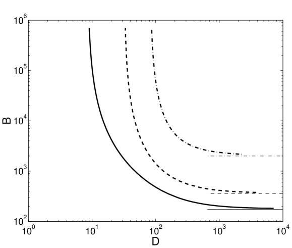
Values of the $B$ and $D$ parameters (in logarithmic scales) that give a zero cosmological constant with the ansatz of Eq. (51). The hidden gauge group is SU(5), and $m=10^{-10}M_{P}$ for all the curves. The solid line corresponds to $q+\bar{q}=1$ and $\delta_{GS}=45/192\pi^{2}$, the dashed line to $q+\bar{q}=2.5$ and $\delta_{GS}=120/192\pi^{2}$ and the dash-dotted line to $q+\bar{q}=3.5$ and $\delta_{GS}=150/192\pi^{2}$. The thin lines show the corresponding lower bound on $B$ obtained from Eq. (60).

The sizes of $K^{\prime}$ and $K^{\prime\prime}$ at the minimum are

$$|K^{\prime}| \sim O(10)<18$$ (52)

$$|K^{\prime\prime}| \sim O(100)|K^{\prime}|\;\;.$$ (54)

The second equation satisfies the bound Eq. (39), while the first one has implications on the size of the soft terms as we shall shortly see.

Concerning the size of the different terms in the potential, it is remarkable how, for small (big) values of the $D$ ($B$) parameter it is the $F_{\varphi}$ term the one that dominates over $F_{S}$ in the potential and therefore cancels the $3|W|^{2}$. Given that $K^{\prime}<18$ that means that in this region of the parameter space (see the discussion after Eq. (42))

$$\xi^{2}=\frac{3}{4}\left(1-\sqrt{1-\frac{4}{3}\frac{q+\bar{q}}{N_{c}}}\right)^{2}\;\;.$$ (55)

As $B$ decreases (i.e. $D$ increases) the size of both $F$ terms becomes comparable and, eventually, the value of $\xi^{2}$ tends to a constant value given by $(q+\bar{q})/N_{c}$. This can be understood from Eq. (51) in the asymptotic regime of “small” $B$ (see Fig. 1). Defining $\varepsilon\equiv e^{-B(\sqrt{{\rm Re}S_{min}}-\sqrt{S_{0}})}$ we have in this regime

$$K_{np}|_{min} \sim \frac{D\varepsilon}{B\sqrt{{\rm Re}S_{min}}}\;\;,$$ (56)

$$K^{\prime}_{np}|_{min} \sim \frac{-D\varepsilon}{{\rm Re}S_{min}}\;\;,$$ (57)

$$K^{\prime\prime}_{np}|_{min} \sim \frac{BD\varepsilon}{({\rm Re}S_{min})^{3/2}}\;\;,$$ (58)

where the subscript $min$ denotes values at the minimum. We can now evaluate $f(\xi^{2})$, which is given by

$$f(\xi^{2})=1-\frac{2K^{\prime}}{\delta_{GS}K^{\prime\prime}}\sim 1+\frac{8\sqrt{{\rm Re}S_{min}}}{\delta_{GS}B}\ .$$ (59)

Imposing the limit of Eq. (35), $f(\xi^{2})<3N_{c}/[4(q+\bar{q})]$, we get a lower bound on $B$, which is the one shown in Fig. 1 for each example,

$$B\geq\frac{8\sqrt{{\rm Re}S_{min}}}{\delta_{GS}\left(\frac{3N_{c}}{4(q+\bar{q})}-1\right)}\sim\frac{96\sqrt{{\rm Re}S_{min}}}{1-12\delta_{GS}}\;\;.$$ (60)

It can also be seen in Fig. 1 that $B$ approaches asymptotically this bound, and therefore $f(\xi^{2})$ will tend to a constant value in this limit. Using Eq. (33) we finally obtain that $\xi^{2}$ goes to an asymptotic value given by $(q+\bar{q})/N_{c}$. Using Eq. (46) this means that the ratio $q_{\phi}m_{F}/m_{D}$ tends to $1$. In fact, since $|K^{\prime}|<18$ in these particular models, this same equation tells us that $q_{\phi}m_{F}/m_{D}$ approaches $1$ from below. In other words, we are in a scenario where the scalar soft masses are dominated by the $D$-term (see the discussion at the end of section III). All this is illustrated in Fig. 2 for the same three cases presented in Fig. 1.

FIG. 2.:

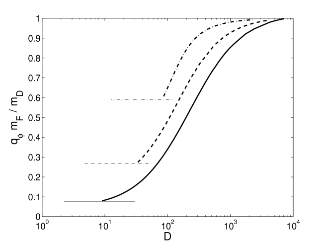
Plot of $q_{\phi}m_{F}/m_{D}$ vs $D$, with $B$ fixed to the values given by the previous figure. Same cases as before. The thin lines show the corresponding lower bound on $q_{\phi}m_{F}/m_{D}$ derived from Eq. (35).

The left hand limit of each curve is determined by the corresponding value of $\xi^{2}$ given by Eq. (55), that is corresponds to $V_{0}=0$ driven by $F_{\varphi}$, whereas as we move in the parameter space towards larger (smaller) values of $D$ ($B$) the $F_{S}$ term contributes more to the cancellation of the cosmological constant until we reach the constant value defined by $\xi^{2}=(q+\bar{q})/N_{c}$. Moreover the ratio $q_{\phi}m_{F}/m_{D}$ tends to its maximum value. Therefore this is an ansatz for $K_{np}$ for which we get the different possibilities for cancelling the cosmological constant, generically with the soft scalar masses dominated by their $D$ contribution.

V Conclusions

Four-dimensional superstring constructions frequently present an anomalous $U(1)_{X}$, which induces a Fayet-Iliopoulos (F-I) D-term. On the other hand SUSY breaking through gaugino condensation is a desirable feature of string scenarios. The interplay between these two facts is not trivial and has important phenomenological consequences, especially concerning the size and type of the soft breaking terms. Previous analyses [5, 6, 7], based on a global SUSY picture, led to contradictory results regarding the relative contribution of the F and D terms to the soft terms.

In this paper we have examined this issue, generalizing the work of ref. [6] to SUGRA, which is the appropriate framework in which to deal with effective theories coming from strings. We have extended the formulation of the F-I term made in [6] to the SUGRA case, as well as considered the complete SUGRA potential in the analysis. This allows to properly implement the cancellation of the cosmological constant (something impossible in global SUSY), which is crucial for a correct treatment of the soft breaking terms. Moreover this condition yields powerful constraints on the Kähler potential, which leads to definite predictions on the relative size of the contributions to the soft terms. In particular we obtain the following hierarchy of masses

$$m_{\lambda}^{2}\ll m_{F}^{2}<m_{D}^{2}\;\;,$$ (61)

where $m_{F}^{2}$, $m_{D}^{2}$ are the contributions from the F and D terms, respectively, to the soft scalar masses, and $m_{\lambda}^{2}$ are the gaugino masses. These results amend those obtained in ref. [6]. The last inequality could be reversed if $K^{\prime}$, i.e. the derivative of the Kähler potential with respect to the dilaton at the minimum, is large ($\stackrel{{\scriptstyle>}}{{{}_{\sim}}}20$). This is not surprising, since in this way the F-I scale (which is proportional to $K^{\prime}$) can be made comparable to $M_{P}$, so that the role of gravity as the messenger of the (F-type) SUSY breaking is not overriden by the “gauge mediated” (D-type) SUSY breaking associated to the F-I term. This situation cannot be excluded, but in our opinion it is unlikely to happen. The first inequality in (61) is rather worrying since it poses a problem of naturality. Namely, given that gaugino masses must be compatible with their experimental limits, the scalar masses must be much higher than 1 TeV, leading to unnatural electroweak breaking. This conclusion seems inescapable in this context.

Finally, we have illustrated all our results with explicit examples, in which the dilaton is stabilized by a gaugino condensate and non-perturbative corrections to the Kähler potential, keeping a vanishing cosmological constant. There it is shown how the various contributions to the soft terms are in agreement to the hierarchy expressed in Eq. (61).

REFERENCES

- [1] J.P. Derendinger, L.E. Ibáñez and H.P. Nilles, Phys. Lett. B155 (1985) 65; M. Dine, R. Rohm, N. Seiberg and E. Witten, Phys. Lett. B156 (1985) 55.
- [2] M. Green and J. Schwarz, Phys. Lett. B149 (1984) 117.
- [3] M. Dine, N. Seiberg and E. Witten, Nucl. Phys. B289 (1987) 589.
- [4] J.A. Casas, E.K. Katehou and C. Muñoz, Nucl. Phys. B317 (1989) 171.
- [5] P. Binétruy and E. Dudas, Phys. Lett. B389 (1996) 503.
- [6] N. Arkani-Hamed, M. Dine and S. Martin, Phys. Lett. B431 (1998) 329.
- [7] G. Dvali and A. Pomarol, Nucl. Phys. B522 (1998) 3.
- [8] L.E. Ibáñez and G.G. Ross, Phys. Lett. B332 (1994) 100.
- [9] P. Binétruy and P. Ramond, Phys. Lett. B350 (1995) 49; P. Binétruy, S. Lavignac, P. Ramond, Nucl. Phys. B477 (1996) 353; P. Binétruy, N. Irges, S. Lavignac, P. Ramond Phys. Lett. B403 (1997) 38; J.K. Elwood, N. Irges and P. Ramond, Phys. Lett. B413 (1997) 322; N. Irges, S. Lavignac, P. Ramond, Phys. Rev. D58 (1998) 35003; Z. Lalak, Nucl. Phys. B521 (1998) 37; S.F. King and A. Riotto, hep-ph/9806281.
- [10] V. Jain and R. Shrock, Phys. Lett. B352 (1995) 83.
- [11] E. Dudas, S. Pokorski and C.A. Savoy, Phys. Lett. B356 (1995) 45; E. Dudas, C. Grojean, S. Pokorski and C.A. Savoy, Nucl. Phys. B481 (1996) 85.
- [12] E.J. Chun and A. Lukas, Phys. Lett. B387 (1996) 99; K. Choi, E.J. Chun and H. Kim, Phys. Lett. B394 (1997) 89.
- [13] R.N. Mohapatra and A. Riotto, Phys. Rev. D55 (1997) 1137 and Phys. Rev. D55 (1997) 4262.
- [14] A.E. Nelson and D. Wright, Phys. Rev. D56 (1997) 1598.
- [15] A.E. Faraggi and J.C. Pati, hep-ph/9712516.
- [16] S.H. Shenker, Proceedings of the Cargese School on Random Surfaces, Quantum Gravity and Strings, Cargese (France), 1990.
- [17] T. Banks and M. Dine, Phys. Rev. D50 (1994) 7454.
- [18] J.A. Casas, Phys. Lett. B384 (1996) 103; P. Binetruy, M.K. Gaillard and Y.-Y. Wu, Nucl. Phys. B481 (1996) 109.
- [19] T. Barreiro, B. de Carlos and E.J. Copeland, Phys. Rev. D57 (1998) 7354.