Matching of $U_{L}(3)\otimes U_{R}(3)$ and $SU_{L}(3)\otimes SU_{R}(3)$ Chiral Perturbation Theories.

P. Herrera-Siklódy

Departament d’Estructura i Constituents de la Matèria
Facultat de Física, Universitat de Barcelona
Diagonal 647, E-08028 Barcelona, Spain
and
I. F. A. E.

Abstract

The heavy singlet field is integrated out from the $U_{L}(3)\otimes U_{R}(3)$ Chiral Perturbation Theory and it is shown how its effects on the low-energy dynamics are reduced to effective vertices for the light mesons. The results are matched against the standard $SU_{L}(3)\otimes SU_{R}(3)$ Chiral Perturbation Theory in order to establish the relations between the coupling constants from both theories to one-loop level accuracy.

PACS: 11.10 Hi, 11.30 Rd, 12.39 Fe

Keywords: $\eta^{\prime}$, Chiral Perturbation Theory, matching.

Introduction

In the low-energy sector, the relevant degrees of freedom in QCD are the Goldstone bosons [1] associated to the spontaneous breaking of the chiral symmetry: $SU_{L}(3)\otimes SU_{R}(3)\rightarrow SU_{V}(3)$. This octet of Goldstone bosons is identified with the eight lightest pseudoscalar particles: the pions, the kaons and the $\eta$; their low-energy interactions are well described in terms of the $SU(3)$ Chiral Perturbation Theory or $\chi PT^{[SU(3)]}$ [2, 3, 4]. The model offers good predictions for energies below a cut-off that is usually set at $M_{\rho}\simeq 770MeV$.

On the other hand, the classical axial symmetry is also broken, but through an anomaly, so it does not generate a ninth Goldstone boson. Nevertheless, the effects of the axial anomaly [5, 6, 7] are suppressed in $1/N_{c}$, where $N_{c}$ is the number of colors. This means that, in the large-$N_{c}$ limit, one can assume a wider scheme containing nine Goldstone bosons (the pseudoscalar octet plus the $\eta^{\prime}$), associated to the spontaneous symmetry breaking $U_{L}(3)\otimes U_{R}(3)\rightarrow U_{V}(3)$ [8, 9]. The corresponding $U(3)$ Chiral Perturbation Theory $\chi PT^{[U(3)]}$ has been described in [10, 11, 12, 13].

The relevant point for this paper is that both theories provide a good description of the lowest energy range: the smaller theory is the low-energy limit of the bigger one. In the low-momenta region, the predictions of observables must coincide. This strong requirement sets the matching conditions and dictates the relation between the coupling constants of both theories.

The ninth field $\eta_{0}$ in $\chi PT^{[U(3)]}$ corresponds essentially to the $\eta^{\prime}$, whose mass $M_{\eta^{\prime}}$ is heavier than the typical octet mass. According to the decoupling theorem [14], if the energy cut-off is reduced quite below the value of $M_{\eta^{\prime}}$, the heavy field will decouple from the lightest octet fields. The dynamics of these remaining fields can then be described by a low-energy theory where the heavy degree of freedom does not appear explicitly: its effects are reduced to effective vertices for the light fields. At the end of the process, we are left with a theory where the relevant degrees of freedom are the octet fields. Its predictions must match those from $\chi PT^{[SU(3)]}$.

In this particular case — $\chi PT^{[U(3)]}$ and $\chi PT^{[SU(3)]}$—, the matching is enormously simplified by the symmetries in both theories. Once the $\eta_{0}$ field has been integrated out, the resulting theory has the same operator structure than $\chi PT^{[SU(3)]}$. This will spare us the painful selection and evaluation of observables that would be required in general for the matching [15]. In this case, the matching can be performed at the effective Lagrangian level [3].

The singlet field is not an actual physical particle, but a mixing of the $\pi_{0}$, the $\eta$ and the heavy $\eta^{\prime}$ [16] instead. Strictly speaking, the field to be integrated out is $\eta^{\prime}$, but the resulting theory would not have the $SU(3)$ symmetry. Furthermore, $M_{0}^{2}\simeq M_{\eta^{\prime}}^{2}$ is a very good approximation, because the large singlet mass is a consequence of the anomaly and not of the mixing. Therefore, the mixing effects will be neglected and $\eta^{\prime}$ will be identified with $\eta_{0}$. On the other hand, the assumption $M_{\eta^{\prime}}\gg M_{octet}$ may not seem numerically justified, since $M_{\eta^{\prime}}\sim 2M_{\eta}$. Both approximations are nevertheless strongly supported by the good results that have been obtained in $\chi PT^{[SU(3)]}$.

The leading-order Lagrangian and its one-loop effective action

The nine Goldstone bosons are introduced in the $U(3)$ Lagrangian by means of a unitary 3 $\times$ 3 matrix $\tilde{U}$:

$$\tilde{U}=\exp\left(i\sum_{\alpha=0}^{8}\frac{\lambda_{\alpha}\phi_{\alpha}}{f}\right),\qquad\mbox{where}\quad\{\lambda_{\alpha}\}_{\alpha=0,...,8}\quad\mbox{are the $U(3)$ generators.}\quad$$

The 3$\times$3 quark mass matrix ${\cal M}$ always appears in two combinations of $\tilde{\chi}=2\tilde{B}{\cal M}$:

$$\tilde{M}=\tilde{U}^{\dagger}{\tilde{\chi}}+{\tilde{\chi}}\tilde{U},\qquad\tilde{N}=\tilde{U}^{\dagger}{\tilde{\chi}}-{\tilde{\chi}}\tilde{U},\quad\mbox{where}\quad{\cal M}=\left(\begin{array}[]{ccc}m_{u}&0&0\\ 0&m_{d}&0\\ 0&0&m_{s}\end{array}\right).$$ (4)

The $U(3)$ theory requires two simultaneous expansions: the usual one, in powers of $p^{2}/f^{2}$ and $M^{2}/f^{2}$, and the large-$N_{c}$ expansion, in powers of $1/N_{c}$. A simple analysis of the particle masses [17, 16, 18] leads to the following choice: $p^{2}\sim m_{q}\sim\frac{1}{N_{c}}\sim\delta$. The expansion in $\delta$ is the consistent way of working in $\chi PT^{[U(3)]}$. Any calculation must be given to a certain ${\cal O}(\delta)$ accuracy; in each case, the relevant terms in the Lagrangian will in general mix different orders in momenta. One of the most interesting features in this way of counting is the fact that both the leading-order ${\cal O}(\delta)$ and the next-to-leading-order ${\cal O}(\delta^{2})$ contribution are tree level. Any loop contribution is suppressed by a factor $M^{2}/f^{2}\sim\delta^{2}$, so the one-loop diagrams involving leading-order vertices introduce corrections of ${\cal O}(\delta^{3})$ or less.

The leading-order Lagrangian is ${\cal O}(\delta)$:

$${\cal L}_{\delta}=\frac{3}{2}\,v_{02}\,\eta_{0}^{2}+\frac{\tilde{f}^{2}}{4}\left(\langle D_{\mu}\tilde{U}^{\dagger}D^{\mu}\tilde{U}\rangle+\langle\tilde{M}\rangle\right),$$

where $\eta_{0}=\phi_{0}$ is the singlet field and brackets stand as usual for trace over flavor indices. $\tilde{B}$, $\tilde{f}$ and $v_{02}$ are the free parameters of the theory to be fixed by experimental data. The tildes are used to distinguish them from the ones that appear in the $SU(3)$ model. According to the $N_{c}$-counting rules, $\tilde{f}\sim{\cal O}(N_{c}^{1/2})$, $\tilde{B}\sim{\cal O}(1)$ and $v_{02}\sim{\cal O}(N_{c}^{-1})$.

The corresponding one-loop effective action can be evaluated with the background field method. The fields are decomposed into a background classical value $\tilde{U}_{c}$ and some quantum fluctuation $\Sigma$:

$$\tilde{U}=\tilde{u}^{\dagger}\Sigma\tilde{u}\,,\;\;\;\tilde{U}_{c}=\tilde{u}^{\dagger}\tilde{u}\,,\;\;\;\Sigma=\exp{\left(i\sum_{\alpha=0}^{8}\lambda_{\alpha}\Delta_{\alpha}\right)}.$$

(Notice that the $\Delta_{0}$ fluctuations factorise in a natural way from the rest of the fields because $\lambda_{0}$ commutes with everything). The action is then expanded in powers of the fluctuations up to quadratic terms and the path integral is performed over all possible configurations of these fluctuations. At the end, the effective action will include the bare Lagrangian ${\cal L}_{\delta}$ itself, its one-loop corrections, that are ${\cal O}(\delta^{3}$), and the appropriate ${\cal O}(\delta^{2}$) and ${\cal O}(\delta^{3}$) counterterms required to cancel the divergences.

$$\Gamma_{eff}^{one-loop}[\tilde{U}_{c}]=\int{\rm d}^{4}x\left({\cal L}^{r}_{\delta}(\tilde{U}_{c})+{\cal L}^{r}_{\delta^{2}}(\tilde{U}_{c})+{\cal L}^{r}_{\delta^{3}}(\tilde{U}_{c})\right)+\;\mbox{finite one-loop corrections.}$$

${\cal L}^{r}_{\delta^{n}}$ stands for the renormalized Lagrangian of order $\delta^{n}$. Schematically, these Lagrangians are built with the operators associated to the following list of coupling constants (see [13] for the complete list of operators):

$${\cal L}_{\delta^{2}} : v_{31},L_{i}(0)\;\;\;\;i=1,2,3,5,8,9,10,11,12,13,14,15,16.$$

$${\cal L}_{\delta^{3}} : v_{04},v_{12},v_{22},L_{i}(0)\;\;\;\;i=4,6,7,18,19,20.$$

For sufficiently low energies, the heavy field $\eta_{0}$ appears only as a fluctuation and its background value is zero. To ${\cal O}(\Delta^{2})$, the ${\cal O}(\delta$) Lagrangian has then the following structure:

$${\cal L}(\tilde{U})\big{|}_{\eta_{0}=0}\sim{\cal L}(U_{c})+J_{0}\,\Delta_{0}-\frac{1}{2}\,\Delta_{0}\,D_{00}\,\Delta_{0}-\frac{1}{2}\,\Delta_{a}\,D_{ab}\,\Delta_{b}-\Delta_{a}\,D_{a0}\,\Delta_{0},$$ (5)

where repeated indices are to be summed over a, b = 1, …, 8, and $J_{0}$, $D_{00}$, $D_{0a}$ and $D_{ab}$ are functions of $U_{c}=\tilde{U}_{c}\big{|}_{\eta_{0}=0}$. The 9$\times$9 matrix $D$ can be written as:

$$D_{\alpha\beta}=(\tilde{d}_{\mu}\tilde{d}^{\mu}+\tilde{\sigma})_{\alpha\beta}\,\bigg{|}_{\eta_{0}=0},\;\;\alpha,\beta=0,...,8.$$ (6)

The complete expressions for $\tilde{\sigma}$ and $\tilde{d}_{\mu}$ have been given in [13] . The covariant derivative $\tilde{d}_{\mu}$ includes a connection: $(\tilde{d}_{\mu}\Delta)^{\alpha}=\partial_{\mu}\Delta^{\alpha}+\omega^{\alpha\beta}_{\mu}\Delta^{\beta}$, although we will not be concerned about its particular form, because the ${\cal O}(\delta)$ Lagrangian gives $\omega_{0\alpha}=0$ $\forall\alpha$. Similarly, the rest is reduced to $\tilde{\sigma}\big{|}_{\eta_{0}=0}=\sigma$. At the end, the relevant objects are:

$$\begin{array}[]{cc}D_{00}=\partial_{\mu}\partial^{\mu}+\sigma_{00},&\qquad\sigma_{00}=\frac{1}{6}\,\langle\tilde{M}\rangle-3\,v_{02}=M_{0}^{2}+\hat{\sigma},\\ D_{a0}=D_{0a}\;=\;\sigma_{a0}\;=\;\frac{1}{2\sqrt{6}}\,\langle\lambda_{a}\tilde{M}\rangle,\quad a\neq 0,&J_{0}=i\,\frac{\tilde{f}}{2\sqrt{6}}\,\langle\tilde{N}\rangle.\end{array}$$ (9)

Before the integration, it is convenient to diagonalize the quadratic part in (5) by means of a change of variables:

$$\varphi_{a}=\Delta_{a}+(D^{-1})_{ab}D_{b0}\,\Delta_{0},\qquad\varphi_{0}=\Delta_{0}.$$

The resulting expression exhibits a perfect quadratic structure:

$${\cal L}(\tilde{U})\big{|}_{\eta_{0}=0}\simeq{\cal L}(U_{c})+J_{0}\,\varphi_{0}-\frac{1}{2}\,\varphi_{0}\left(D_{00}-D_{0a}(D^{-1})_{ab}D_{b0}\right)\varphi_{0}-\frac{1}{2}\,\varphi_{a}\,D_{ab}\,\varphi_{b}.$$ (10)

The effective action is given by integrating over all configurations for the fluctuations ($\varphi_{0}$ and $\varphi_{a}$’s):

$$e^{\,i\Gamma_{eff}^{[U(3)]}[U]}=\int[{\rm d}\varphi_{0}]\prod_{a=1}^{8}[{\rm d}\varphi_{a}]\,e^{i{\int{\rm d}^{4}x\,{\cal L}(\tilde{U})}}\,{\bigg{|}}_{\eta_{0}=0}\,.$$

In order to get a more friendly notation, the subscript $c$ has been dropped. In what follows, every $U$ or $\tilde{U}$ is to be understood as made of classical fields whose value is set to the background value.

A straightforward Gaussian integration leads to

$$\Gamma_{eff}[U] = \frac{1}{2}\int{\rm d}^{4}x\,J_{0}\,D_{00}^{-1}\,J_{0}+\frac{i}{2}\,{\rm Tr}\,\ln\,D_{00}-\frac{i}{2}\,{\rm Tr}\left(D_{00}^{-1}D_{0a}(D^{-1})_{ab}D_{b0}\right)$$ (11)

$$+ \int{\rm d}^{4}x\,{\cal L}_{U(3)}(U)+\frac{i}{2}\,{\rm Tr}\,\ln D_{ab}+{\cal O}(\delta^{3}).$$

The last term (where the sub-indices have been kept to recall that it is an 8$\times$8 matrix) contains all the one-loop diagrams with particles from the octet circulating in the internal lines. The three terms in the first line are due to diagrams containing one and two heavy internal lines and will be analyzed below. All these one-loop contributions contain divergences that are absorbed by the appropriate counterterms, so we will be dealing with one-loop renormalized coupling constants.

The first term in the right-hand side of (11) corresponds to a tree graph with light external lines and a heavy internal $\eta_{0}$ propagator that is seen as an $SU(3)$ effective vertex in the low-energy theory (fig. 1 a). This term was already analyzed in [3, 19]. The operator $D_{00}$ can be split into two pieces:

$$D_{00}=D_{o}+\hat{\sigma}.$$ (12)

$D_{o}$ is the free operator of a scalar field with mass $M_{0}$: $D_{o}=\partial_{\mu}\partial^{\mu}+M_{0}^{2}$, and $\hat{\sigma}=\sigma_{00}-M_{0}^{2}$. $\hat{\sigma}$ contains vertices with two or more light fields. Its inclusion in the following calculation would only contribute to ${\cal O}(p^{6})$ vertices, so it will not be considered.

If the cut-off is small compared to $M_{0}^{2}$, or in the limit of large distances, the interaction can be assumed to be local and the following integral can be approximated by a delta function:

$$D_{00}(x)\simeq\int\frac{{\rm d}^{4}p}{(2\pi)^{4}}\,e^{-ip\cdot x}\frac{1}{M_{0}^{2}-p^{2}}\simeq\frac{1}{M_{0}^{2}}\,\delta^{4}(x).$$

Thus the contribution due to this term is:

$$\Gamma_{tree}[U]=-\frac{\tilde{f}^{2}}{48\,M_{0}^{2}}\,\int{\rm d}^{4}x\,\langle\tilde{N}\rangle^{2}.$$ (13)

The other pieces originate in one-loop graphs. The identity (12) can be used to expand the trace of the logarithm in (11):

$$\frac{i}{2}\,{\rm Tr}\,\ln D_{00}=\frac{i}{2}\,{\rm Tr}\,\ln(D_{o}+\hat{\sigma})\simeq\frac{i}{2}\,{\rm Tr}\,\ln D_{o}+\frac{i}{2}\,{\rm Tr}\left(D_{o}^{-1}\hat{\sigma}\right)-\frac{i}{4}\,{\rm Tr}\left(D_{o}^{-1}\hat{\sigma}D_{o}^{-1}\hat{\sigma}\right)+...$$ (14)

The first term in (14) is a constant that can be ignored. The second and third terms correspond to one-loop diagrams with one and two internal $\eta_{0}$ lines, respectively (fig.1 b and c).

The $\eta_{0}$ tadpole term, that we shall call $\Gamma_{\eta_{0}}$, gives:

$$\Gamma_{\eta_{0}}[U] = \frac{i}{2}\,{\rm Tr}\left(D_{o}^{-1}\hat{\sigma}\right)\;=\;\frac{i}{2}\,\Delta_{0}(0)\int{\rm d}^{4}x\,\hat{\sigma}(x)$$ (15)

$$= -\frac{1}{6}\,(M_{0}^{2}\lambda_{\epsilon}+\frac{M_{0}^{2}}{32\pi^{2}}\,\ln\frac{M_{0}^{2}}{\mu^{2}})\int{\rm d}^{4}x\,\left(\langle\tilde{M}\rangle-18\,v_{02}-6\,M_{0}^{2}\right),$$

where $\lambda_{\epsilon}$ is a divergent term and is given in the appendix (23). This and the other divergent pieces that will come up in (16) and (17) are just part of the one-loop renormalization of the leading-order U(3) theory.

$\Gamma_{\eta_{0}\eta_{0}}$ contains all the diagrams with two internal $\eta_{0}$. For the sake of clearness, the details of the calculation have been relegated to the appendix. The resulting contribution is:

$$\Gamma_{\eta_{0}\eta_{0}}[U] = -\frac{i}{4}\,{\rm Tr}\left(D_{o}^{-1}\hat{\sigma}D_{o}^{-1}\hat{\sigma}\right)\;=\;-\frac{1}{2}\,(k_{00}+\lambda_{\epsilon})\int{\rm d}^{4}x\,\hat{\sigma}(x)^{2}$$ (16)

$$= -\frac{1}{72}\,(k_{00}+\lambda_{\epsilon})\int{\rm d}^{4}x\,\left(\langle\tilde{M}\rangle-18\,v_{02}-6\,M_{0}^{2}\right)^{2}.$$

$k_{00}$ is given in (25). Obviously, the constant terms in (15) and (16) can be dropped out.

Finally, the third term in (11) corresponds to one-loop diagrams with one internal $\eta_{0}$ and one internal $\pi$ (unless otherwise stated, pion is used in a generic sense, meaning any particle from the octet). In the $U(3)$ theory, the pions can take higher values of momentum and these modes must be integrated out, too. This integration can be understood in two different steps: the integration of heavy $\eta_{0}$’s and of high momenta pions yields an $SU(3)$ bare vertex with pion external legs and one internal pion line with low momenta. The integration of these remaining low-momentum modes gives the $SU(3)$ tadpole renormalization of this new vertex (fig. 1 d).

The reader should again refer to the appendix for the details of the calculation. The result in this case is (P labels the octet mesons):

$$\Gamma_{\eta_{0}\pi}[U] = -\frac{i}{2}\,{\rm Tr}\left((D^{-1})_{ab}\sigma_{a0}D^{-1}_{00}\sigma_{0b}\right)=-\sum_{P}(\lambda_{\epsilon}+k_{0P})\int{\rm d}^{4}x\,\sigma_{0P}(x)^{2}$$ (17)

$$= -\frac{1}{12}\left(\lambda_{\epsilon}+\frac{1}{32\pi^{2}}\ln\,\frac{M_{0}^{2}}{\mu^{2}}\right)\int{\rm d}^{4}x\,\left(\langle\tilde{M}^{2}\rangle-\frac{1}{3}\langle\tilde{M}\rangle^{2}\right)$$

$$+ \frac{1}{24\cdot 32\pi^{2}}\sum_{P}a_{P}\int{\rm d}^{4}x\,\langle\tilde{M}\lambda_{P}\rangle^{2},$$

where $k_{0P}$ is given in (25) and $a_{P}$ is defined as:

$$a_{P}=\frac{M_{P}^{2}}{M_{0}^{2}-M_{P}^{2}}\,\ln\frac{M_{P}^{2}}{M_{0}^{2}}.$$

The last term in (17) reflects the explicit breaking of the $U(3)$ symmetry. This contribution could be neglected if all quark masses were small enough: the corrections depend on the ratio $M_{P}^{2}/M_{0}^{2}$. It will be taken into account, however, because $M_{K}^{2}$ and $M_{\eta}^{2}$ are not that small when compared to $M_{0}^{2}$. This happens because $m_{s}\gg m_{u}$, $m_{d}$. For simplicity, we shall assume that $m_{u},m_{d}=0$ but $m_{s}\neq 0$. In this limit, $M_{\pi}=a_{\pi}=0$ and $\chi$ turns out to be a very simple matrix; as a consequence,

$$\langle\tilde{M}\lambda_{i}\rangle=0\quad\mbox{for}\;i=1,\,2,\,3,\qquad\qquad\lambda_{8}=\frac{1}{\sqrt{3}}\left(I-\frac{3}{2\,B\,m_{s}}\,\chi\right),$$ (18)

$$\sum_{i=4}^{7}\langle\tilde{M}\lambda_{i}\rangle^{2}=2\langle\tilde{M}^{2}\rangle-\frac{2}{3}\,\langle\tilde{M}\rangle^{2}-\langle\tilde{M}\lambda_{8}\rangle^{2}.\qquad\qquad$$

Recall that the $\eta-\eta^{\prime}$ mixing effects are neglected, so $\lambda_{\eta}\simeq\lambda_{8}$. At the end, one can write:

$$\sum_{P}a_{P}\,\langle\tilde{M}\lambda_{P}\rangle^{2}\simeq 2\,a_{K}\,\langle\tilde{M}^{2}\rangle+(\frac{a_{\eta}}{3}-a_{K})\,\langle\tilde{M}\rangle^{2}+{\cal O}(\frac{M_{\pi}^{2}}{M_{0}^{2}})+{\cal O}(p^{6}).$$

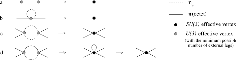
Figure 1: The effects of heavy internal modes reduce to effective vertices in the $SU(3)$ theory.

Matching

The low-energy one-loop effective action (11) is given by the sum of (13), (15), (16) and (17):

$$\Gamma^{U(3)}_{eff}[U] = \int{\rm d}^{4}x\,{\cal L}^{r}_{U(3)}(U)+\;\mbox{finite corrections involving one loop of pions}-\frac{\tilde{f}^{2}}{48\,M_{0}^{2}}\,\langle\tilde{N}\rangle^{2}$$ (19)

$$+ \frac{M_{0}^{2}}{6\cdot 32\pi^{2}\tilde{f}^{2}}\,\ln\frac{M_{0}^{2}}{\mu^{2}}\int{\rm d}^{4}x\,\langle\tilde{M}\rangle-\frac{1}{72}\,k_{00}\int{\rm d}^{4}x\,\left(\langle\tilde{M}\rangle^{2}-12\,(M_{0}^{2}+3v_{02})\,\langle\tilde{M}\rangle\right)$$

$$- \frac{1}{12\cdot 32\pi^{2}}\ln\,\frac{M_{0}^{2}}{\mu^{2}}\int{\rm d}^{4}x\,\left(\langle\tilde{M}^{2}\rangle-\frac{\langle\tilde{M}\rangle^{2}}{3}\right)+\frac{1}{24\cdot 32\pi^{2}}\sum_{P}a_{P}\int{\rm d}^{4}x\,\langle\tilde{M}\lambda_{P}\rangle^{2}.$$

This effective action describes the same system as the $SU(3)$ one-loop effective action [3]:

$$\Gamma^{SU(3)}_{eff}[U] = \int{\rm d}^{4}x\,{\cal L}_{SU(3)}(U)+\frac{i}{2}\,{\rm Tr}\,\ln D_{ab}$$ (20)

$$= \int{\rm d}^{4}x\,{\cal L}^{r}_{SU(3)}(U)+\;\mbox{finite corrections involving one loop of pions}.$$

The matching conditions require physical quantities to give identical results in both cases. In a general case, one would be forced to compare the observables that stem from both theories. At tree-level, for instance, both theories give a prediction for the mass of the pion, and they must be equal: $B(m_{u}+m_{d})=\tilde{B}(m_{u}+m_{d})$. This implies that $\tilde{B}=B+{\cal O}(\delta^{2})$.

In this case, however, one needs not go all the way down to observables. The operator structure of both effective actions is identical, allowing for a much easier procedure:

$$\Gamma^{SU(3)}_{eff}[U]=\Gamma^{U(3)}_{eff}[U].$$ (21)

One can safely replace $\tilde{B}$ by $B$ everywhere in (19) except in the original ${\cal O}(\delta)$ Lagrangian, because $\tilde{B}=B+{\cal O}(\delta^{2})$. By doing this, all the corrections involving one loop of pions in (20) and (19) become identical and cancel out in (21). Both theories must indeed present identical behaviors in the IR region. In particular, the IR non-analyticities that occur in these pion-loop terms in the chiral limit are exactly the same and the matching calculation is IR finite [20].

All the ${\cal O}(p^{4})$ terms —except for the last one— can then be easily written in terms of the usual $SU(3)$ operators that include the external source $\chi=2B{\cal M}$:

$$\langle M^{2}\rangle=O_{8}+2\,O_{12},\qquad\langle M\rangle^{2}=O_{6},\qquad\langle N\rangle^{2}=O_{7},$$

where:

$$\begin{array}[]{ll}O_{6}=\langle U^{{\dagger}}\chi+\chi^{{\dagger}}U\rangle^{2},&O_{7}=\langle U^{{\dagger}}\chi-\chi^{{\dagger}}U\rangle^{2},\\ O_{8}=\langle U^{{\dagger}}\chi U^{{\dagger}}\chi+\chi^{{\dagger}}U\chi^{{\dagger}}U\rangle,&O_{12}=\langle\chi^{{\dagger}}\chi\rangle.\end{array}$$

Finally, by directly comparing the structures and identifying the factors preceding each operator on both sides of (21), one obtains the following relations between the renormalized $SU(3)$ coupling constants (plain) and the $U(3)$ ones (tilded), in terms of physical quantities :

$$f = \tilde{f},$$

$$B = \tilde{B}(\mu)+\frac{\tilde{B}(\mu)}{48\pi^{2}f_{\pi}^{2}}\left(M_{\eta^{\prime}}^{2}\,\ln\frac{M_{\eta^{\prime}}^{2}}{\mu^{2}}+(M_{\eta}^{2}-2\,M_{K}^{2})\,(\ln\frac{M_{\eta^{\prime}}^{2}}{\mu^{2}}+1)\right),$$

$$L_{6}^{r}(\mu) = \tilde{L}_{6}^{r}(\mu)+\frac{1}{72\cdot 32\pi^{2}}\left(\ln\frac{M_{\eta^{\prime}}^{2}}{\mu^{2}}+\,a_{\eta}-3\,a_{K}-1\right)+{\cal O}(\frac{M_{\pi}^{2}}{M_{\eta^{\prime}}^{2}}),$$

$$L_{7}^{r}(\mu) = \tilde{L}_{7}^{r}(\mu)-\frac{f_{\pi}^{2}}{48\,M_{\eta^{\prime}}^{2}},$$

$$L_{8}^{r}(\mu) = \tilde{L}_{8}^{r}(\mu)-\frac{1}{12\cdot 32\pi^{2}}\left(\ln\frac{M_{\eta^{\prime}}^{2}}{\mu^{2}}-a_{K}\right)+{\cal O}(\frac{M_{\pi}^{2}}{M_{\eta^{\prime}}^{2}}),$$

$$H_{2}^{r}(\mu) = \tilde{L}_{12}^{r}(\mu)-\frac{1}{6\cdot 32\pi^{2}}\left(\ln\frac{M_{\eta^{\prime}}^{2}}{\mu^{2}}-a_{K}\right)+{\cal O}(\frac{M_{\pi}^{2}}{M_{\eta^{\prime}}^{2}}),$$

$$L_{i}^{r}(\mu) = \tilde{L}_{i}^{r}(\mu),\qquad\mbox{ for i = 1, 2, 3, 4, 5, 9, 10},$$

$$H_{1}^{r}(\mu) = \tilde{L}_{11}^{r}(\mu).$$ (22)

One can check that the dependence on the renormalization parameter $\mu$ is the same on both sides of the equalities. This parameter has been introduced to deal with the UV divergences in both theories; a convenient choice of its value will avoid the growth of large logs and the breakdown of perturbation theory. The typical scale used in $\chi PT^{[SU(3)]}$, $\mu\simeq M_{\rho}$, will do the job.

Concluding remarks

It is worth emphasizing the running of $\tilde{B}$, because this is a special characteristic of $\chi PT^{[U(3)]}$:

$$\mu\frac{\partial\tilde{B}^{r}}{\partial\mu} = \tilde{B}^{r}\frac{v_{02}}{16\,\pi^{2}f^{2}}\,.$$

The correction to $\tilde{B}$ exhibits the typical $M_{\eta^{\prime}}^{2}$ correction to the light masses that arises from the integration of a heavy scalar field. This results in a paradox —the so-called naturalness problem— when one tries to push the calculation to the limit $M_{\eta^{\prime}}\rightarrow\infty$. The contradiction is easily solved in this case: if $\eta^{\prime}$ were very heavy, the nonet theory that we started from would be wrong.

As expected from the Appelquist-Carrazone theorem, all the effects from the integrated heavy particle are either suppressed in powers of $M_{\eta^{\prime}}^{2}$ and/or can be re-absorbed in the coupling constants of the lower theory. The correction to $L_{7}$, for instance, originates in the momentum expansion of a perfectly analytical tree graph. In contrast, loop graphs contributions incorporate non-analytical $\ln M_{\eta^{\prime}}$ terms — that could be never obtained through a Taylor expansion.

The value of the coupling constants in the $SU(3)$ theory are relatively well known, so this work offers a first estimate of the unknown $U(3)$ parameters. A numerical check can be done in the case of $L_{8}$. At $\mu=M_{\rho}$, $L_{8}(M_{\rho})=(0.9\pm 0.3)\cdot 10^{-3}$ and the value predicted in (22) is $\tilde{L_{8}}(M_{\rho})=(1.2\pm 0.3)\cdot 10^{-3}$. This is too small compared to the value found in [16], where $\tilde{L}_{8}$ was estimated to be $(1.3-1.6)\cdot 10^{-3}$, but the correction goes in the right direction.

$L_{7}$ has always been related to $\eta^{\prime}$. This has produced some confusion on the $N_{c}$-power counting of this parameter [3, 19]. The problem disappears by noticing that the $1/N_{c}$ expansion must be implemented in the $U(3)$ context: the $N_{c}\rightarrow\infty$ limit has no meaning in the $SU(3)$ theory, because the very first consequence of assuming the large-$N_{c}$ limit is that there are nine Goldstone bosons instead of eight. One might however wish to keep track of the $N_{c}$ counting for each $SU(3)$ coupling because it justifies why some of them are smaller than the rest and thus negligible. It can be seen in (22) that all corrections but the correction for $\tilde{L}_{7}$ are either ${\cal O}(1)$ or suppressed in $\delta^{2}$, so the $N_{c}$ counting for the $SU(3)$ couplings stays the same as in $U(3)$, except for one case: $\tilde{L}_{7}$ is ${\cal O}(1)$, but its correction is ${\cal O}(N_{c}^{2})$, so $L_{7}$ ends up being ${\cal O}(N_{c}^{2})$. The numerical value of this correction is $-0.2\cdot 10^{-3}$, which has indeed the same order of magnitude of the present value of $L_{7}=(-0.4\pm 0.2)\cdot 10^{-3}$.

Appendix

The tadpole term (15) reduces to $\Delta_{P}(0)$, the Feynman propagator of a scalar particle of mass $M_{P}$ in $z=0$.

$$i\Delta_{P}(0)=-2\,M_{P}^{2}\,\lambda_{\epsilon}-\frac{M_{P}^{2}}{16\pi^{2}}\,\ln\,\frac{M_{P}^{2}}{\mu^{2}},\quad\mbox{where}\quad\lambda_{\epsilon}=\frac{\mu^{2\epsilon}}{2\,(4\pi)^{2}}\left(\frac{1}{\epsilon}+\gamma-\ln 4\pi-1\right).$$ (23)

The traces in (16) and (17) involve a particular kind of integral and can be written in terms of a function $J_{P0}(z)=-i\Delta_{0}(z)\Delta_{P}(z)$:

$$-\frac{i}{2}\,{\rm Tr}\left(D_{ab}^{-1}\sigma_{a0}D_{o}^{-1}\sigma_{0b}\right) = \frac{1}{2}\int{\rm d}^{4}x\,{\rm d}^{4}y\,J_{0P}(x-y)\,\sigma_{0P}(x)\,\sigma_{0P}(y),$$

$$-\frac{i}{4}\,{\rm Tr}\left(D_{o}^{-1}\hat{\sigma}D_{o}^{-1}\hat{\sigma}\right) = \frac{1}{4}\int{\rm d}^{4}x\,{\rm d}^{4}y\,J_{00}(x-y)\,\hat{\sigma}(x)\,\hat{\sigma}(y),$$ (24)

In momentum space and using dimensional regularization, $D=4+2\epsilon$,

$$J_{0P}(s) = \int{\rm d}^{4}z\;e^{ipz}\;J_{0P}(z)=-i\int\frac{{\rm d}^{D}q}{(2\pi)^{D}}\;\frac{1}{M_{0}^{2}-q^{2}+i\varepsilon}\;\frac{1}{M_{P}^{2}-(p-q)^{2}+i\varepsilon}$$

$$= -2\,\lambda_{\epsilon}-2\,k_{0P}+\bar{J}_{0P}(s),$$

where $s=p^{2}$ is the external momentum and

$$k_{0P}=\frac{1}{32\pi^{2}}\left(\ln\frac{M_{0}^{2}}{\mu^{2}}+\frac{M_{P}^{2}}{M_{P}^{2}-M_{0}^{2}}\,\ln\,\frac{M_{P}^{2}}{M_{0}^{2}}\right),\qquad k_{00}=\frac{1}{32\pi^{2}}\left(\ln\frac{M_{0}^{2}}{\mu^{2}}+1\right).$$ (25)

$\bar{J}_{0P}(s)$ is some function of s, $M_{0}^{2}$ and $M_{P}^{2}$, but we shall omit it, because it does not contribute to the low-energy limit:

$$J_{0P}(s)\simeq J_{0P}(0)+{\cal O}(\frac{p^{2}}{M_{0}^{2}})=-2\,\lambda_{\epsilon}-2\,k_{0P}+{\cal O}(\frac{p^{2}}{M_{0}^{2}}).$$

In this limit, the integrals (24) reduce to a very simple form:

$$-\frac{i}{2}\,{\rm Tr}\left(D_{ab}^{-1}\sigma_{a0}D_{o}^{-1}\sigma_{0b}\right) = -\sum_{P}\left(k_{0P}+\lambda_{\epsilon}\right)\int{\rm d}^{4}x\;\sigma_{0P}(x)^{2},$$

$$-\frac{i}{4}\,{\rm Tr}\left(D_{o}^{-1}\hat{\sigma}D_{o}^{-1}\hat{\sigma}\right) = -\frac{1}{2}\left(k_{00}+\lambda_{\epsilon}\right)\int{\rm d}^{4}x\;\hat{\sigma}(x)^{2}.$$

References

• [1] J. Goldstone, Nuovo Cimento 19 (1961) 154.
• [2] S. Weinberg Physica 96A (1979) 327.
• [3] J. Gasser and H. Leutwyler, Nucl. Phys. B250 (1985) 465.
• [4] A review on the subject: A. Pich, Rept. Prog. Phys. 58 (1995) 563.
• [5] S. L. Adler, Phys. Rev. 177 (1969) 2426.
• [6] J. S. Bell and R. Jackiw, Nuovo Cimento 60A (1969) 47.
• [7] S. L. Adler and W. A. Bardeen, Phys. Rev. 182 (1969) 1517.
• [8] E. Witten Nucl. Phys. B156 (1979) 269.
• [9] G. Veneziano, Nucl. Phys. B117 (1974) 519; B159 (1979) 213.
• [10] P. Di Vecchia and G. Veneziano, Nucl. Phys. B171 (1980) 253; P. Di Vecchia et al., Nucl. Phys. B181 (1981) 318.
• [11] E. Witten, Ann. Phys. 128 (1980) 363.
• [12] C. Rosenzweig, J. Schechter and T. Trahern, Phys. Rev. D21 (1980) 3388.
• [13] P. Herrera-SiklΓ³dy et al., Nucl. Phys. B497 (1997) 345.
• [14] T. Appelquist, J. Carrazone, Phys. Rev. D11 (1975) 2856.
• [15] A. Pich, Effective Field Theory, course given in Les Houches Summer School 1997, hep-ph/9806303, to be published by Elsevier Science B.V.
• [16] P. Herrera-SiklΓ³dy et al., Phys. Lett. B419 (1998) 326.
• [17] H. Leutwyler, Phys. Lett. B374 (1996) 163.
• [18] R. Kaiser, H. Leutwyler, hep-ph/9806336.
• [19] G. Ecker et al., Nucl. Phys. B321 (1989) 311; S. Peris, E. de Rafael, Phys. Lett. B348 (1995) 539.
• [20] H. Georgi, in Advanced School on Effective Theories, edited by F. Cornet and M. J. Herrero (World Scientific, Singapore, 1997), p. 88.; H. Georgi, Annu. Rev. Part. Sci 43 (1993) 209.