Abstract

A brief discussion of the elastic $\pi\pi$ scattering amplitude to two loops in chiral perturbation theory is given. Some technical details of the evaluation of two-loop diagrams are addressed, and results relevant for the pionium decay are presented.

1. INTRODUCTION

In this talk I’ll briefly summarize the results of our two-loop calculation of the $\pi\pi$ amplitude[1, 2]. Also, some technical issues[3], useful for the evaluation of two-loop graphs in a number of processes, are discussed.

The investigation of the $\pi\pi$ interaction is of particular interest at present, because there are several experiments which will bring new information after a long break in the experimental activity. Of special interest in this workshop is the pionium experiment DIRAC (PS 212) at CERN[4] which aims at measuring the lifetime of the $\pi^{+}\pi^{-}$ atomic bound state. The relevant quantity there is the difference of the I=0 and I=2 $s$-wave scattering lengths, $a^{0}_{0}-a^{2}_{0}$. The forthcoming K_l4 data from the KLOE detector starting to operate at DA$\Phi$NE in Frascati will also add substantially to our understanding of the low-energy $\pi\pi$ interaction. Similar data from BNL (E865) are already coming to analysis[5]. An attempt at IUCF to see pionium production in the reaction $pd\rightarrow^{3}\!\!{\it He}\,\pi^{+}\pi^{-}$ has given only the upper limit, 1 $pb$, for the production cross section[6]. The standard method to measure $\pi\pi$ scattering at high energies is to study the pion induced pion production, $\pi N\rightarrow\pi\pi N$. At low energies, however, the extraction of $\pi\pi$ information from this reaction is complicated by the fact that there one-pion-exchange does not necessarily dominate.

From theoretical point of view the interest in the $\pi\pi$ interaction is well motivated. The question is to what extent our picture of spontaneously broken chiral symmetry is valid. The $\pi\pi$ studies will provide a test. The technique employed here, chiral perturbation theory (ChPT), is a systematic approach to build the chiral symmetry of QCD into the low-energy amplitudes. The tool to do that is the effective Lagrangian, so the $\pi\pi$ studies provide also a testing ground for the effective field theory techniques. Another aspect of particular interest recently is the size of the quark-antiquark vacuum condensate[7, 8]. According to the standard picture the condensate should be “large”, whereas the, so called, generalized ChPT allows for a “small” value for the condensate. Generally speaking, these two values correspond respectively to a small, about 0.2, and a large, around 0.3, value for the isoscalar $s$-wave scattering length.

Another technique to address the $\pi\pi$ problem is also making progress, namely the lattice approach. The lattice method can give estimates of both the vacuum condensate and the $\pi\pi$ scattering lengths. However, some questions remain, especially the role of the dynamical quarks, or the relatively high pion mass still involved. In any case, some encouraging results have already been obtained[9].

ChPT is a systematic expansion of the Green functions in terms of external momenta and quark masses. A number of theoretical assumptions are invoked. These include that the chiral symmetry of QCD is spontaneously broken, and that the low-energy singularities of the theory are generated by the Goldstone degrees of freedom[10, 11].

In this talk the $\pi\pi$ interaction will be discussed in chiral $SU(2)\times SU(2)$. A technical remark referring to the evaluation of some loop diagrams is included. Then a summary of the results relevant for the pionium system will be given together with some prospects for future work.

2. EFFECTIVE LAGRANGIAN

The chiral effective Lagrangian can be written as

$${\cal L}_{\rm eff}={\cal L}_{2}+{\cal L}_{4}+{\cal L}_{6}+...$$ (1)

where the indices refer to the chiral counting, the number of derivatives of the pion field or twice the power of the quark mass terms. The two-loop calculation involves the evaluation of the amplitude up to and including terms ${\cal O}(p^{6})$. As a consequence, the part ${\cal L}_{6}$ appears at tree level, the part ${\cal L}_{4}$ at both tree- and one-loop level and finally the piece ${\cal L}_{2}$ at tree-, 1-loop and 2-loop level. It is convenient to adopt for ${\cal L}_{2}$ the form

$${\cal L}_{2}=\frac{F^{2}}{4}\left\langle D_{\mu}U\,D^{\mu}U^{\dagger}+U\chi^{\dagger}+U^{\dagger}\chi\right\rangle$$ (2)

where the brackets $\langle\,\rangle$ refer to trace over the flavour indices and $F$ is the pion decay constant in the chiral limit. It is convenient to work with the field

$$U = \sigma+i\frac{\mbox{\boldmath$\phi$}}{F}\;,\;\;\;\;\sigma^{2}+\frac{\mbox{\boldmath$\phi$}^{2}}{F^{2}}={\bf\mbox{1}}\;\;,$$

$$\phi = \left(\mbox{$\begin{array}[]{cc}\pi^{0}&\sqrt{2}\pi^{+}\\ \sqrt{2}\pi^{-}&-\pi^{0}\end{array}$}\right)=\phi^{i}\tau^{i}\;,$$ (5)

$$\chi = 2B(\hat{m}{\bf\mbox{1}}+ip),\;\;\hat{m}=\frac{1}{2}(m_{u}+m_{d})$$ (6)

where $p$ is an external pseudoscalar source. The second constant appearing in ${\cal L}_{2}$, $B$, is proportional to the vacuum condensate. The next order Lagrangian is of the type

$${\cal L}_{4} = \sum^{4}_{i=1}l_{i}P_{i}+\dots$$ (7)

where the $l_{i}$’s are the low-energy constants required by the one-loop renormalization of the $\pi\pi$ amplitude. The explicit form of the terms $P_{i}$ can be found e.g. in ref.[12]. The form of ${\cal L}_{6}$ has been given in ref.[13].

3. TWO-LOOP INTEGRALS

A number of processes contain the same topologies in two-loop graphs:

• vector and axialvector 2-point functions

• $\pi\rightarrow e\nu\gamma$

• scalar and vector form factors of the pion

• $\pi\pi\rightarrow\pi\pi$

• $\gamma\gamma\rightarrow\pi\pi$

As an example let us consider the fish graph in figure 1 contributing to $\pi\pi$ scattering.

Figure 1: The fish diagram. The filled circles denote vertices from the effective Lagrangian ${\cal L}_{2}$. The internal lines stand for scalar propagators with mass 1.

The contribution is proportional to

$$\int\frac{d^{d}l_{1}}{i(2\pi)^{d}}\int\frac{d^{d}l_{2}}{i(2\pi)^{d}}\,\prod_{i=1}^{4}\frac{1}{D_{i}}$$

where

$$D_{1} = 1-l_{1}^{2},$$

$$D_{2} = 1-(Q-l_{1})^{2},$$

$$D_{3} = 1-l_{2}^{2},$$

$$D_{4} = 1-(l_{2}+l_{1}-p_{1})^{2},$$

$$Q = p_{1}+p_{2},\;\;Q^{2}=s.$$

The integration over $l_{2}$ gives the loop–function $J(\bar{t})$ with $\bar{t}=(p_{1}-l_{1})^{2},\;\;\;$ ($w=d/2-2$)

$$J(\bar{t})=C(w){\Gamma(-w)}\int_{0}^{1}dx\,[1-\bar{t}x(1-x)]^{w},$$ (8)

which can be represented in the form

$$J(\bar{t})=\int_{4}^{\infty}\frac{[d\sigma]}{\sigma-\bar{t}}.$$ (9)

The measure is

$$[d\sigma]=\frac{C(w)\Gamma(3/2)}{\Gamma(3/2+w)}(\frac{\sigma}{4}-1)^{w}\beta\;d\sigma,\;\;{\rm where}$$

$$C(w)=\frac{1}{(4\pi)^{2+w}},\;\;\;\beta=(1-4/\sigma)^{1/2}.$$

In the limit $d\rightarrow 4$ this gives

$$\lim_{w\rightarrow 0}\;[d\sigma]=\frac{\beta}{16\pi^{2}}\;d\sigma.$$

The emerging subdivergence is subtracted $J(\bar{t})=J(0)+\bar{J}(\bar{t})$ and we have for the fish diagram $J(s)J(0)+V(s)$ where

$$V=\int_{4}^{\infty}\frac{[d\sigma]}{\sigma}\int\frac{d^{d}l_{1}}{i(2\pi)^{d}}\,\frac{\bar{t}}{D_{1}D_{2}(\sigma-\bar{t})}\,.$$ (10)

Using the Feynman parametrization and integrating over $l_{1}$ yields in the limit $w\rightarrow 0$ a triple integral for the finite part, $V_{f}$. The imaginary part of $V_{f}$ can be constructed using the standard techniques and the result

$${\rm Im}\,V_{f}(s)=\frac{\pi}{(16\pi^{2})^{2}}\left[3\rho+\ln\frac{1-\rho}{1+\rho}-\frac{1}{s\rho}\ln^{2}\frac{1-\rho}{1+\rho}\right]$$

follows. A function with the proper cut structure and $s\rightarrow 0,\infty$ behaviour is[2, 3]

$$V_{f}(s)=\frac{1}{(16\pi^{2})^{2}}\left[\left(3-\frac{\pi^{2}}{3s\rho^{2}}\right)f+\frac{1}{2\rho^{2}}f^{2}-\frac{1}{3s\rho^{4}}f^{3}+6+\frac{\pi^{2}}{6}\right],$$ (11)

where

$$f = \rho\left\{\ln\frac{1-\rho}{1+\rho}+i\pi\right\},$$

$$\rho = \sqrt{1-4/s},\;\;\;\;s>4\;.$$

The remarkable thing here is that even such graphs can be evaluated analytically.

4. PION-PION AMPLITUDE

The $\pi\pi$ amplitude can be written in the form

$$T^{ik;lm} = \delta^{ik}\delta^{lm}A(s,t,u)+\delta^{il}\delta^{km}A(t,s,u)$$

$$+ \delta^{im}\delta^{kl}A(u,t,s)$$

where to two loop order

$$A(s,t,u)=\hskip 8.5359pt{\it x_{2}}\left[s-1\right]\hfill\;\;\;\;\;\;\;\;\;\;\;\;\;\;\;\;\;\;\;\;\;\;\;\;\;\;\;$$

$$+{\it x_{2}}^{2}\left[b_{1}+b_{2}s+b_{3}s^{2}+b_{4}(t-u)^{2}\right]$$

$$+{\it x_{2}}^{2}\left[F^{(1)}(s)+G^{(1)}(s,t)+G^{(1)}(s,u)\right]$$

$$+{\it x_{2}}^{3}\left[b_{5}s^{3}+b_{6}s(t-u)^{2}\right]$$

$$+{\it x_{2}}^{3}\left[F^{(2)}(s)+G^{(2)}(s,t)+G^{(2)}(s,u)\right]\,\!$$

$$+O({\it x_{2}}^{4})$$ (12)

and

$${\it x_{2}}=\frac{M_{\pi}^{2}}{F_{\pi}^{2}}.$$

Unitarity fixes the analytically nontrivial functions $F^{(1)},G^{(1)}$ of the one-loop piece and $F^{(2)},G^{(2)}$ for the two-loop amplitude[1]. The leading order result (${\cal O}(x_{2})$) is due to Weinberg[14] and the one-loop piece (${\cal O}(x_{2}^{2})$) due to Gasser and Leutwyler[15, 12]. In the isospin basis

$$T^{0}(s,t) = 3\,A(s,t,u)+A(t,u,s)+A(u,s,t)$$

$$T^{1}(s,t) = A(t,u,s)-A(u,s,t)$$

$$T^{2}(s,t) = A(t,u,s)+A(u,s,t)$$

The relevant quantity for pionium decay is the charge exchange amplitude

$$T(\pi^{+}\pi^{-}\rightarrow\pi^{0}\pi^{0})=\frac{1}{3}\left[T^{0}(s,t)-T^{2}(s,t)\right]$$

and the decay rate

$${\rm RATE}\propto(a^{0}_{0}-a^{2}_{0})^{2}.$$

The two-loop amplitude involves six low-energy constants (the one-loop level has four $l$’s, and the two-loop piece six $r$’s[1, 2]. They appear, however, in six independent combinations, $b_{1,...,6}$.) To clarify the structure of these constants $b_{4}$ is taken as an example:

$$b_{4}=\frac{1}{2}\,l_{2}^{r}-\frac{1}{6}L-\frac{1}{16{\pi}^{2}}\frac{5}{36}\;\;\;\;\;\;\;\;\;\;\;\;\;\;\;\;\;\;\;\;\;\;\;$$

$$+{x_{2}}\left\{{\vrule height=8.6pt,width=0.0pt,depth=8.6pt}\right.\!\!\frac{1}{16{\pi}^{2}}\left[{\vrule height=8.6pt,width=0.0pt,depth=8.6pt}\right.\!\!\frac{10}{9}\,l_{1}^{r}+\frac{4}{9}\,l_{2}^{r}-\frac{5}{9}\,l_{4}^{r}+\frac{47}{216}L$$

$$\;\;\;\;\;\;\;\;\;\;\;\;+\frac{17}{3456}+\frac{1}{16{\pi}^{2}}\frac{1655}{2592}\!\!\left.{\vrule height=8.6pt,width=0.0pt,depth=8.6pt}\right]$$

$$+2\,l_{2}^{r}\,l_{4}^{r}-\frac{1}{6}\left[k_{1}+4k_{2}+k_{4}\right]+r_{4}^{r}\!\left.{\vrule height=8.6pt,width=0.0pt,depth=8.6pt}\right\}$$ (13)

where

$$L = \frac{1}{16\pi^{2}}\ln{\frac{M_{\pi}^{2}}{\mu^{2}}}$$

$$k_{i} = (4\,l_{i}^{r}(\mu)-\gamma_{i}L)L\;;$$ (14)

$$l_{i}^{r} = \frac{\gamma_{i}}{32\pi^{2}}\left(\bar{l}_{i}+\ln\frac{M_{\pi}^{2}}{\mu^{2}}\right).$$

In the framework of the generalized ChPT the $\pi\pi$ amplitude has been evaluated[16] in dispersive manner. The pieces fixed by unitarity, $F$’s and $G$’s, agree with our results. The main difference is that the Lagrangian approach taken here allows for determining the structure of the constants $b_{i}$ of the polynomial part in terms of the pion mass and the low-energy constants of both ${\cal O}(p^{4})$ and ${\cal O}(p^{6})$. The knowledge of the mass dependence makes it possible to compare results with the lattice calculations where unphysical value for the pion mass is still needed[17].

5. RESULTS

For comparison with experiment numerical values for the constants $\bar{l}_{1,...,4}$ and $r$’s will be needed. The resonance saturation with the main contributions from the scalar and vector mesons can be used for the $r$’s. The influence of these values is small to the final amplitudes. The main effect comes from the constants $\bar{l}_{i}$ which show up already at order $x_{2}^{2}$. A detailed study of $\bar{l}_{i}$’s with constraints from the Roy equations is on the way[18], and with those values one can hope to reach a precision of 2–3 % for the $s$-wave scattering lengths. The values used in ref.[2] were taken from the K_l4 analysis of ref.[19] or from the $\pi\pi$ $d$-wave scattering lengths fixing $\bar{l}_{1}$ and $\bar{l}_{2}$, i.e. two sets of values were taken for the numerical comparisons. For the Set I we have[19]:

$$\bar{l}_{1}=-1.7,\;\;\;\bar{l}_{2}=6.1,\;\;\;\bar{l}_{3}=2.9,\;\;\;\bar{l}_{4}=4.3$$

and Set II:

$$\bar{l}_{1}=-1.5,\;\;\;\bar{l}_{2}=4.5\;\;\;\bar{l}_{3}\;{\rm and}\;\bar{l}_{4}\;\mbox{{\rm as in SET I.}}$$

The phase shift difference $\delta^{0}_{0}-\delta^{1}_{1}$ for these sets of low-energy constants has been given in figure 2 as a function of the centre-of-mass energy.

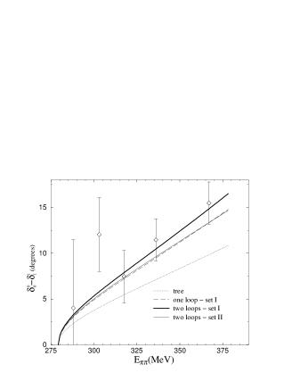
Figure 2: The phase shift difference $\delta^{0}_{0}-\delta^{1}_{1}$ for two different sets of low-energy constants. The data points are from ref.[20].

For the $s$-wave scattering length we get

$$a^{0}_{0} = \frac{7{\it x_{2}}}{32\pi}\left\{1-{\it x_{2}}\left[\frac{9}{2}L+\mbox{analytic}\right]\right.$$ (15)

$$\left.\hskip 41.25648pt+{\it x_{2}}^{2}\left[\frac{58}{7}k_{1}+\frac{96}{7}k_{2}+5k_{3}+\frac{11}{2}k_{4}+\frac{1697}{84}\frac{L}{16\pi^{2}}+\mbox{analytic}\right]\right.$$

$$\left.\hskip 27.0301pt+O({\it x_{2}}^{3})\;\;\right\}$$

and numerically at scale $\mu$=1 GeV for the isoscalar $s$-wave scattering length and the difference of the $s$-wave scattering lengths with Set I

$$a_{0}^{0} = \overbrace{0.156}^{\mbox{tree}}+\overbrace{0.039+0.005}^{\mbox{1~{}loop}}+\overbrace{0.013+0.003+0.001}^{\mbox{2~{}loops}}\;=\;\overbrace{0.217}^{\mbox{total}},$$

$$\hskip 54.06006ptL\hskip 21.33955pt\mbox{anal.}\hskip 31.2982ptk_{i}\hskip 28.45274ptL\hskip 22.76228pt\mbox{anal.}$$

$$a_{0}^{0}-a_{0}^{2} = 0.201+0.036+0.006+0.012+0.003+0.001\;=\;0.258.$$

$$\hskip 54.06006ptL\hskip 21.33955pt\mbox{anal.}\hskip 31.2982ptk_{i}\hskip 28.45274ptL\hskip 22.76228pt\mbox{anal.}$$

In this case it is seen that the nonanalytic terms dominate both the one-loop and the two-loop corrections. The value for $a^{0}_{0}-a^{2}_{0}$ corresponding to Set II is 0.250. The experimental figure obtained by using the universal curve is 0.29$\pm$0.04[1]. Using dispersion sum rules the constants $b_{3,...,6}$ have been determined[21, 22] and within the quoted errors these values are consistent with Set II.

6. CONCLUSIONS AND FUTURE PROSPECTS

The corrections in the loop expansion for the scattering length difference, $a^{0}_{0}-a^{2}_{0}$, seem to be converging quite rapidly, about 20 % correction from the tree level to one-loop calculation and 6 % from one-loop to two-loop (calculated with Set I). Therefore, in near future we can expect the precision of the calculation to reach 2-3 % level which is significant in strong interaction physics. This implies that the analyses of $\pi\pi$ data will have to be made with extreme care. This is the challenge for the K_e4 experiments in Brookhaven and Frascati, and the pionium experiment at CERN.

Acknowledgements

I would like to thank Jürg Gasser for useful comments on the write-up. Also, partial support from the EU-TMR programme, contract CT98-0169, is acknowledged.

References

• [1] J. Bijnens, G. Colangelo, G. Ecker, J. Gasser and M.E. Sainio, Phys. Lett. B374 (1996) 210.
• [2] J. Bijnens, G. Colangelo, G. Ecker, J. Gasser and M.E. Sainio, Nucl. Phys. B508 (1997) 263; (E) ibid. B517 (1998) 639.
• [3] J. Gasser and M.E. Sainio, Eur. Phys. J. C (in press); hep-ph/9803251.
• [4] B. Adeva et al., CERN/SPSLC 95-1 (1994).
• [5] D. Lazarus et al., Brookhaven proposal BNL-AGS-E865.
• [6] A.C. Betker et al., Phys. Rev. Lett. 77 (1996) 3510.
• [7] N.H. Fuchs, H. Sazdjian and J. Stern, Phys. Lett. B269 (1991) 183.
• [8] H. Leutwyler, Nucl. Phys. A623 (1997) 169c.
• [9] S. Aoki et al., Nucl. Phys. Proc. Suppl. 60A (1998) 14;
M. Fukugita, Y. Kuramashi, M. Okawa, H. Mino and A. Ukawa, Phys. Rev. D52 (1995) 3003.
• [10] S. Weinberg, Physica 96A (1979) 327.
• [11] H. Leutwyler, Ann. Phys. (N.Y.) 235 (1994) 165.
• [12] J. Gasser and H. Leutwyler, Ann. Phys. (N.Y.) 158 (1984) 142.
• [13] H.W. Fearing and S. Scherer, Phys. Rev. D53 (1996) 315.
• [14] S. Weinberg, Phys. Rev. Lett. 17 (1966) 616.
• [15] J. Gasser and H. Leutwyler, Phys. Lett. B125 (1983) 325.
• [16] M. Knecht, B. Moussallam, J. Stern and N.H. Fuchs, Nucl. Phys. B457 (1995) 513.
• [17] G. Colangelo, Phys. Lett. B395 (1997) 289.
• [18] J. Gasser, these proceedings.
• [19] J. Bijnens, G. Colangelo and J. Gasser, Nucl. Phys. B427 (1994) 427.
• [20] L. Rosselet et al., Phys. Rev. D15 (1977) 574.
• [21] M. Knecht, B. Moussallam, J. Stern and N.H. Fuchs, Nucl. Phys. B471 (1996) 445.
• [22] L. Girlanda, M. Knecht, B. Moussallam and J. Stern, Phys. Lett. B409 (1997) 461.