BARI-TH/309-98
Super-Kamiokande atmospheric neutrino data,
zenith distributions, and three-flavor oscillations

Abstract

We present a detailed analysis of the zenith angle distributions of atmospheric neutrino events observed in the Super-Kamiokande (SK) underground experiment, assuming two-flavor and three-flavor oscillations (with one dominant mass scale) among active neutrinos. In particular, we calculate the five angular distributions associated to sub-GeV and multi-GeV $\mu$-like and $e$-like events and to upward through-going muons, for a total of 30 accurately computed observables (zenith bins). First we study how such observables vary with the oscillation parameters, and then we perform a fit to the experimental data as measured in SK for an exposure of 33 kTy (535 days). In the two-flavor mixing case, we confirm the results of the SK Collaboration analysis, namely, that $\nu_{\mu}\leftrightarrow\nu_{\tau}$ oscillations are preferred over $\nu_{\mu}\leftrightarrow\nu_{e}$, and that the no oscillation case is excluded with high confidence. In the three-flavor mixing case, we perform our analysis with and without the additional constraints imposed by the CHOOZ reactor experiment. In both cases, the analysis favors a dominance of the $\nu_{\mu}\leftrightarrow\nu_{\tau}$ channel. Without the CHOOZ constraints, the amplitudes of the subdominant $\nu_{\mu}\leftrightarrow\nu_{e}$ and $\nu_{e}\leftrightarrow\nu_{\tau}$ transitions can also be relatively large, indicating that, at present, current SK data do not exclude sizable $\nu_{e}$ mixing by themselves. After combining the CHOOZ and SK data, the amplitudes of the subdominant transitions are constrained to be smaller, but they can still play a nonnegligible role both in atmospheric and other neutrino oscillation searches. In particular, we find that the $\nu_{e}$ appearance probability expected in long baseline experiments can reach the testable level of $\sim 15\%$. We also discuss earth matter effects, theoretical uncertainties, and various aspects of the statistical analysis.

I Introduction

The Super-Kamiokande (SK) water-Cherenkov experiment [1] has recently confirmed [2, 3, 4], with high statistical significance, the anomalous flavor composition of the observed atmospheric neutrino flux, as compared with theoretical expectations [5, 6]. The flavor anomaly had been previously found in Kamiokande [7, 8] and IMB [9], and later in Soudan2 [10], but not in the low-statistics experiments NUSEX [11] and Fréjus [12].

The recent SK data have also confirmed earlier Kamiokande indications [8] for a dependence of the flavor anomaly on the lepton zenith angle [3, 4], which is correlated with the neutrino pathlength. The features of this dependence are consistent with the hypothesis of neutrino oscillations, which represents the most natural (and perhaps exclusive) explanation of the data [4]. The oscillation hypothesis is also consistent with other recent atmospheric neutrino data, namely, the finalized sample of Kamiokande upward-going muons [13], the latest muon and electron data from Soudan2 [14], and the samples of stopping and through-going muons in MACRO [15].

The SK atmospheric $\nu$ measurements, which are described in detail in several papers [16, 2, 3, 4], conference proceedings [17, 18, 19], and theses [20, 21, 22], demand the greatest attention, not only for their intrinsic importance, but also for their interplay with other oscillation searches, including solar $\nu$ experiments [23] and long baseline oscillation experiments at reactors [24, 25, 26] and accelerators [27, 28, 29, 30, 31]. In this work, we contribute to these topics by performing a comprehensive, quantitative, and accurate study of the SK atmospheric $\nu$ data in the hypothesis of three-flavor mixing among active neutrinos. We also include, within the same framework, the recent data from the CHOOZ reactor experiment [24, 25].

More precisely, we consider the five SK angular distributions associated to sub-GeV and multi-GeV $\mu$-like and $e$-like events [2, 3] and to upward through-going muons [18, 19], for a total of 30 accurately computed observables (5+5+5+5+10 zenith bins). First we study how such observables vary with the oscillation parameters, and then we fit them to the experimental data as measured in SK for an exposure of 33 kTy (535 days) [4, 18].

In the two-flavor mixing case, we confirm the results of the SK Collaboration analysis, namely, that $\nu_{\mu}\leftrightarrow\nu_{\tau}$ oscillations are preferred over $\nu_{\mu}\leftrightarrow\nu_{e}$, and that the no oscillation case is excluded with high confidence. In the three-flavor mixing case, we perform our analysis with and without the additional constraints imposed by the CHOOZ reactor experiment. In both cases, the analysis favors a dominance of the $\nu_{\mu}\leftrightarrow\nu_{\tau}$ channel. Without the CHOOZ constraints, the amplitudes of the subdominant $\nu_{\mu}\leftrightarrow\nu_{e}$ and $\nu_{e}\leftrightarrow\nu_{\tau}$ transitions can also be relatively large, indicating that, at present, current SK data do not exclude sizable $\nu_{e}$ mixing by themselves. After combining the CHOOZ and SK data, the amplitudes of the subdominant transitions become smaller, but we show that they can still play a nonnegligible role both in atmospheric, solar, and long baseline laboratory experiments.

The plan of our paper is as follows. In Section II we discuss the 30 SK observables used in the analysis, as well as the CHOOZ measurement. In Section III we set the notation for our three-flavor oscillation framework. The two-flavor subcases are studied in Sec. IV. In Sec. V we perform the three-flavor analysis of SK data (with and without the CHOOZ constraints) and discuss the results, especially those concerning $\nu_{e}$ mixing. In Sec. VI we study the implications of our analysis for the neutrino oscillation phenomenology. We conclude our work in Sec. VII, and devote Appendixes A and B to the discussion of technical details related to our calculations and to the statistical analysis.

Some of our previous results on two- and three-flavor oscillations of solar [32, 33, 34], atmospheric [35, 36, 37, 38], laboratory [39, 40] neutrino experiments and their combinations [41, 42, 43, 44] will be often referred to in this work. In particular, the $3\nu$ analyses in [32, 36, 37, 38, 39] summarize the pre-SK situation. However, we have tried to keep this paper as self-contained as possible.

II Expectations and DATA

In this Section we discuss expectations and data for five SK zenith distributions: sub-GeV $e$-like and $\mu$-like, multi-GeV $e$-like and $\mu$-like, and upward-going muons, with emphasis on some critical aspects of both theory and data that are often neglected. Finally, we discuss the CHOOZ reactor results.

A Zenith distributions of neutrinos and leptons

A basic ingredient of any theoretical calculation or MonteCarlo simulation of atmospheric $\nu$ event rates is the flux $\Phi$ of atmospheric neutrinos and antineutrinos as a function of the energy $E_{\nu}$ and of the zenith angle $\Theta$. The flux $\Phi(E_{\nu},\Theta)$ is unobservable in itself, and what is measured is the distribution of leptons $\ell=\mu,e$ after $\nu$ interactions, as a function of the lepton energy $E_{\ell}$ $(<E_{\nu})$ and lepton zenith angle $\theta$ $(\neq\Theta)$.

In Fig. 1 we show the sum of theoretical $\nu$ and $\overline{\nu}$ fluxes, as a function of the neutrino zenith angle $\Theta$, for selected values of the energy $E_{\nu}$ (1, 10, and 100 GeV). The fluxes refer to the calculations of [5] (HKKM’95, solid lines) and [6] (AGLS’96, dots) without geomagnetic corrections (so that the sign of $\cos\Theta$ is irrelevant in this figure). The upper and middle panels refer to muon and electron neutrinos, respectively, while the lower panel shows their ratio. Several interesting things can be learned from this figure. For instance, the often quoted value $(\nu_{\mu}+\overline{\nu}_{\mu})/(\nu_{e}+\overline{\nu}_{e})\simeq 2$ for the muon-to-electron neutrino ratio clearly holds only for low-energy, horizontal neutrinos. This ratio increases rapidly as the neutrino energy increases and as its direction approaches the vertical. In fact, both $\nu_{\mu}$ and $\nu_{e}$ fluxes decrease towards the vertical (see upper and middle panels), where the slanted depth in the atmosphere is reduced; however, $\nu_{e}$’s are more effectively suppressed than $\nu_{\mu}$’s, due to their different parent decay chains. In addition, the greater the energy of the parents, the longer the decay lengths, the stronger the dependence of the $\nu_{\mu}/\nu_{e}$ flux ratio on the slanted depth and thus on the zenith angle $\Theta$. In other words, high-energy, vertical “atmospheric $\nu$ beams” are richer in $\nu_{\mu}$’s and, therefore, are best suited in searches for $\nu_{\mu}\to\nu_{e}$ oscillations, where initial $\nu_{e}$’s represent the “background” (see also [45]). We anticipate that, in fact, multi-GeV data are more effective than lower-energy (sub-GeV) data in placing bounds on $\nu_{\mu}\to\nu_{e}$ transitions. Another consequence of the non-flat $\nu_{\mu}/\nu_{e}$ ratio is the appearance of distortions of the zenith distributions that, although related to vacuum neutrino oscillation, do not depend on neutrino pathlength-to-energy ratio $L/E_{\nu}$ [38]. Finally, notice in Fig. 1 that the good agreement at low energies between the two reported calculations of $\nu_{\mu}/\nu_{e}$ is somewhat spoiled at high energies. This shows that the often-quoted uncertainty of $\pm 5\%$ for the $\nu_{\mu}/\nu_{e}$ ratio, which has been estimated in detail for low energy, integrated fluxes [46], does not necessarily apply to high-energy or differential fluxes. Therefore, also the $\mu/e$ lepton event ratio might suffer of uncertainties larger than $\pm 5\%$ in some energy-angle bins. Our empirical estimate of such errors in the statistical analysis is detailed in Appendix B. More precise estimates of the relative $\nu_{\mu}$ and $\nu_{e}$ flux uncertainties are in progress [47, 48]. A new, ab initio, fully three-dimensional calculation of the atmospheric neutrino flux [49] is also expected to shed light on these issues.

FIG. 1.: Distributions of neutrino fluxes in terms of the neutrino zenith angle $\Theta$, for three representative energies ($E_{\nu}=1$, 10, and 100 GeV). Upper panels: $\nu_{\mu}+\overline{\nu}_{\mu}$ flux. Middle panels: $\nu_{e}+\overline{\nu}_{e}$ flux. Lower panels: $(\nu_{\mu}+\overline{\nu}_{\mu})/(\nu_{e}+\overline{\nu}_{e})$ flux ratio. Solid lines and dots refer to the calculations in [5] (HKKM’95) and [6] (AGLS’96), respectively. In this figure, geomagnetic effects are not reported, and the fluxes are symmetric under $\cos\Theta\to-\cos\Theta$. Notice the increase of the $\nu_{\mu}/\nu_{e}$ ratio with energy and for $|\cos\Theta|\to 1$.

Concerning the overall uncertainty of the theoretical neutrino flux normalization, it is usually estimated to be 20–30%. Most of the uncertainty is associated to the primary flux of cosmic rays hitting the atmosphere. It is important, however, to allow also for energy-angle variations of such normalization (e.g., the SK analysis [4] allows the spectral index to vary within $\pm 0.05$). Our approach to this problem is detailed in Appendix B. Here we want to emphasize that valuable information about the overall flux normalization can be obtained from more precise cosmic ray data from balloon experiments such as BESS [50], CAPRICE [51], and MASS2 [52, 53]. The BESS experiment has recently reported a relatively low flux of cosmic primaries [50], which, as we will see, might represent a serious problem for the oscillation interpretation of the SK data (see also [47, 48]). On the other hand, the MASS2 experiment can also measure the flux of primary protons and secondary muons at the same time [54], and might thus provide soon an important calibration of the theoretical flux calculations [54, 55]. Therefore, it is reasonable to expect, in a few years, a reduction and a better understanding of the overall neutrino flux uncertainty, with obvious benefits for the interpretation of the atmospheric $\nu$ anomaly.

In order to obtain measurable quantities (e.g., the lepton zenith angle distributions), one has to make a convolution of the neutrino fluxes with the differential cross sections and detection efficiencies (see, e.g., [36, 43, 44]). We consider five zenith angle distributions of leptons: sub-GeV muons and electrons, multi-GeV muons and electrons, and upward through-going muons. Concerning the calculation of the first four distributions, we have used the same technique used in [36] for the old Kamiokande multi-GeV distributions. This approach makes use of the energy distributions of parent interacting neutrinos [56]. Concerning upward through-going muons, we improve the approach used in [37] by including the zenith dependence of the SK muon energy threshold as given in [19, 20]; we also use the same SK choice for the parton structure functions (GRV94 [57], available in [58]) and muon energy losses in the rock [59, 20]. For all distributions (SG, MG, and UP$\mu$), we obtain a good agreement with the corresponding distributions simulated by the SK collaboration, as reported in Appendix A (to which we refer the reader for further details).

In short, we can compute five distributions of SK lepton events as a function of the zenith angle $\theta$, namely, sub-GeV $\mu$-like and $e$-like events (5+5 bins), multi-GeV $\mu$-like and $e$-like events (5+5 bins), and upward through-going muons (10 bins), for a total of 30 observables. Few other analyses report explicit calculations of sub-GeV and multi-GeV zenith distributions (see, e.g., [60, 61]) or upward-going muon distributions (see, e.g., [62]) in agreement with the SK simulations. Other authors perform detailed calculations but use a reduced zenith information, as that embedded, e.g., in the up-down lepton rate asymmetry [63] (see, e.g., [64, 65]).

B SK Data: Total and differential rates

The experimental data used in our analysis are reported in Table I and Table II, together with the corresponding expectations as taken from the SK MonteCarlo simulations. The numerical values have been graphically reduced from the plots in [4, 18] and thus may be subject to slight inaccuracies.

Table I reports the zenith angle distributions of sub-GeV and multi-GeV events collected in the SK fiducial mass (22.5 kton) during 535 live days, for a total exposure of 33 kTy. Fully and partially contained multi-GeV muons have been summed. Only single-ring events are considered. The distributions are binned in five intervals of equal width in $\cos\theta$, from $\cos\theta=-1$ (upward going leptons) to $\cos\theta=+1$ (downward going leptons). The total number of events in the full solid angle is also given. The quoted uncertainties for the data points are statistical. The statistical uncertainties associated to the SK MonteCarlo expectations originate from the finite simulated exposure (10 years live time [17]).

Table II reports the differential and total flux of upward through-going muons as a function of the zenith angle. Data errors are statistical only. In this case, there is no statistical error for the SK theoretical estimates, which are derived from a direct calculation [18, 19, 20] and not from a MonteCarlo simulation.

It is useful to display the information in Tables I and II in graphical form. To this purpose, we take the central values of the theoretical expectations in Tables I and II as “units of measure” in each bin. In other words, all $\mu$ and $e$ event rates (either observed, or calculated in the presence of oscillations) are normalized to their standard (i.e., unoscillated) expectations $\mu_{0}$ and $e_{0}$. The following notations distinguish the various lepton samples:

$$\begin{array}[]{ccl}{\rm SG}e&=&\text{sub-GeV\ electrons}\ ,\\ {\rm SG}\mu&=&\text{sub-GeV\ muons}\ ,\\ {\rm MG}e&=&\text{multi-GeV\ electrons}\ ,\\ {\rm MG}\mu&=&\text{multi-GeV\ muons}\ ,\\ {\rm UP}\mu&=&\text{upward\ through-going\ muons}\ ,\\ {\rm MC}&=&\text{theory\ (no\ oscillation)}\ .\end{array}$$

TABLE I.: Super-Kamiokande sub-GeV and multi-GeV $e$-like and $\mu$-like atmospheric neutrino data, compared with the corresponding MonteCarlo simulations in different zenith angle ($\theta$) bins [4]. The numerical values are graphically reduced from the plots in [4, 18]. Units: Number of events. Experimental exposure: 33 kTy, corresponding to 22.5 kton fiducial mass $\times$ 535 live days. Simulated exposure: 10 yr [17]. Errors are statistical only. The Super-Kamiokande MonteCarlo simulations refer to HKKM’95 neutrino fluxes [5].

Event	Bin	$\cos\theta$	Observed	MonteCarlo	Observed	MonteCarlo
sample	No.	range	$e$-like events	$e$-like events	$\mu$-like events	$\mu$-like events
Sub-GeV	1	$[-1.0,\,-0.6]$	$287\pm 16.9$	$209\pm 5.5$	$182\pm 13.5$	$326\pm 6.9$
	2	$[-0.6,\,-0.2]$	$231\pm 15.2$	$206\pm 5.5$	$225\pm 15.0$	$316\pm 6.8$
	3	$[-0.2,\,+0.2]$	$259\pm 16.1$	$220\pm 5.7$	$228\pm 15.1$	$307\pm 6.7$
	4	$[+0.2,\,+0.6]$	$227\pm 15.1$	$216\pm 5.6$	$264\pm 16.2$	$308\pm 6.7$
	5	$[+0.6,\,+1.0]$	$227\pm 15.1$	$198\pm 5.4$	$259\pm 16.1$	$317\pm 6.8$
	total	$[-1.0,\,+1.0]$	$1231\pm 35.1$	$1049\pm 12.4$	$1158\pm 34.0$	$1574\pm 15.2$
Multi-GeV	1	$[-1.0,\,-0.6]$	$50\pm 7.1$	$37\pm 2.3$	$64\pm 8.0$	$114\pm 4.1$
	2	$[-0.6,\,-0.2]$	$56\pm 7.5$	$51\pm 2.7$	$75\pm 8.7$	$132\pm 4.4$
	3	$[-0.2,\,+0.2]$	$70\pm 8.4$	$62\pm 3.0$	$136\pm 11.7$	$173\pm 5.0$
	4	$[+0.2,\,+0.6]$	$74\pm 8.6$	$52\pm 2.8$	$142\pm 11.9$	$139\pm 4.5$
	5	$[+0.6,\,+1.0]$	$40\pm 6.3$	$34\pm 2.2$	$114\pm 10.7$	$111\pm 4.0$
	total	$[-1.0,\,+1.0]$	$290\pm 17.0$	$236\pm 5.9$	$531\pm 23.0$	$669\pm 9.9$

TABLE II.: Super-Kamiokande 535 day data on upward through-going muon fluxes, compared with the corresponding theoretical calculations in different zenith angle ($\theta$) bins [18]. Units: $10^{-13}$ cm^-2 s^-1 sr^-1. The calculated muon fluxes, taken from [18, 19], refer to HKKM’95 neutrino fluxes [5], GRV’94 DIS structure functions [57], and Lohmann muon energy losses in the rock [59]. Errors are statistical only. The numerical values are graphically reduced from the plots in [18, 19].

Bin	$\cos\theta$	Observed	Theoretical
No.	range	$\mu$ flux	$\mu$ flux
1	$[-1.0,\,-0.9]$	$1.03\pm 0.18$	1.25
2	$[-0.9,\,-0.8]$	$1.16\pm 0.18$	1.38
3	$[-0.8,\,-0.7]$	$0.90\pm 0.17$	1.46
4	$[-0.7,\,-0.6]$	$1.62\pm 0.22$	1.57
5	$[-0.6,\,-0.5]$	$1.31\pm 0.18$	1.67
6	$[-0.5,\,-0.4]$	$1.57\pm 0.20$	1.78
7	$[-0.4,\,-0.3]$	$1.59\pm 0.21$	1.93
8	$[-0.3,\,-0.2]$	$2.20\pm 0.25$	2.18
9	$[-0.2,\,-0.1]$	$2.73\pm 0.28$	2.52
10	$[-0.1,\,-0.0]$	$3.42\pm 0.31$	3.03
total	$[-1.0,\,-0.0]$	$1.75\pm 0.07$	1.88

FIG. 2.: Super-Kamiokande data on total lepton events, compared with their theoretical predictions. The numbers of $e$-like and $\mu$-like events are normalized to the central values of the corresponding MonteCarlo (MC) simulations $e_{0}$ and $\mu_{0}$ [4], obtained with HKKM’95 fluxes [5] (as reported in Table I). Error bars of experimental data are statistical; slanted error bars of MC represent $\pm 30\%$ systematics in the common $\mu_{0},e_{0}$ normalization and $\pm 5\%$ systematics in the $\mu_{0}/e_{0}$ ratio. Left panel: Default MC (favors $\nu_{\mu}\to\nu_{e}$ oscillations). Middle panel: MC$\times 1.2$ (favors $\nu_{\mu}\to\nu_{\tau}$ oscillations). Right panel: MC$\times 0.8$ (disfavors $\nu$ oscillations). See the text for details.

Figure 2 compares theory and data for the total lepton rates. The MG$\mu$ data sample is further divided into fully contained (FC) and partially contained (PC) events (notice that MG$e$ events are all FC). The total number of lepton events are displayed in the plane $(\mu/\mu_{0},e/e_{0})$, so that the standard expectations (MC) correspond to the point $(1,1)$ for each data sample. The UP and PC muons have no electron counterpart and are shown in the single variable $\mu/\mu_{0}$ (upper strips). We attach a $\pm 30\%$ common uncertainty to the MC muon and electron rates (large slanted error bar), and allow for a $\pm 5\%$ uncertainty in the $\mu/e$ ratio (small slanted error bar). The three subfigures 2(a), 2(b), and 2(c) correspond to three choices for the theoretical predictions (MC): (a) Standard MC expectations; (b) MC rates multiplied by 1.2; and (c) MC rates multiplied by 0.8.

Figure 2(a) clearly shows that, with respect to the standard MC, SK observes a deficit of muons (stronger for low-energy SG$\mu$ data and weaker for high-energy UP$\mu$ data) and, at the same time, an excess of electrons (both in the SG and MG samples). In the hypothesis of neutrino oscillations, these indications would favor $\nu_{\mu}\to\nu_{e}$ transitions, with a mass square difference low enough to give some energy dependence to the muon deficit. As far as total SK rates are concerned, this is a perfectly viable scenario.

FIG. 3.: Super-Kamiokande distributions of lepton events in terms of the lepton zenith angle $\theta$ ($\cos\theta=-1,0,1$ correspond to upgoing, horizontal, downgoing leptons). From left to right: sub-GeV electrons (SG$e$) and muons (SG$\mu$), multi-GeV electrons (MG$e$) and muons (MG$\mu$), and upward through-going muons UP$\mu$. In each bin, the observed rate $R$ is divided by the expected rate $R_{0}$ in the absence of oscillations, as taken from Tables I and II. Therefore, in this plot Theory=1 with $\pm 30\%$ normalization error, and the deviations of Data (dots) from the flat theoretical expectations show the zenith anomaly at glance.

Figure 2(b) shows how the previous picture changes when one allows for an overall increase of the MC expectations (say, $+20\%$). The relative excess of electrons disappears, while the muon deficit is enhanced. This situation is consistent with $\nu_{\mu}\to\nu_{\tau}$ transitions, which leave the electron rate unaltered. The current SK data link rather strongly $\nu_{\mu}\to\nu_{\tau}$ oscillations to an overall increase of the MC expectations: indeed, a good fit to the SG and MG data samples requires a MC “renormalization” by a factor $\sim 1.16$ [4]. Although this factor is acceptable at present, it might not be so in the future, should the MC predictions become more constrained. In particular, if the recent BESS indications [50] for a relatively low flux of cosmic primaries were confirmed, then one should rather decrease the MC expectations [47, 48].

Figure 2(c) shows the effect of a MC decrease by 20%. In this case one would observe no deficit of muons (and even an excess of UP$\mu$ events) and a $\sim 40\%$ excess of electrons, which cannot be obtained in any known oscillation scenario.

The discussion of Fig. 2 shows that: (i) Theory (no oscillation) and data disagree, even allowing for a MC renormalization; (ii) The oscillation interpretation depends sensitively on the size of the renormalization factor; (iii) If this factor turns out to be $<1$, the oscillation hypothesis is jeopardized; and (iv) It is thus of the utmost importance to calibrate and constrain the theoretical neutrino flux calculations [5, 6] through cosmic ray balloon experiments such as BESS [50], and especially through simultaneous measurements of primary and secondary charged particles as in the forthcoming CAPRICE and MASS2 analyses [54]. All this information would be lost if the popular “$\mu/e$ double ratio” were used. Another piece of information that would be hidden by the double ratio is the fact that, in Fig. 2, the SG and MG data points appear to be very close to each other in the $(\mu/\mu_{0},e/e_{0})$ plane, while it was not so in Kamiokande [35]. We are, however, unable to trace the source of such a difference (which is independent of the MC normalization) between SK and Kamiokande.

Since the total lepton rate information is subject to the above ambiguities, one hopes to learn more from differential rates and, in particular, from the zenith distributions of electrons and muons. These distributions are shown in Fig. 3 where, again, the rates $R$ have been normalized in each bin to the central values of their expectations $R_{0}$ (from Tables I and II). Therefore, the no oscillation case corresponds to “theory = 1” in this figure, with an overall normalization error that we set at $\pm 30\%$. Deviations of the data samples (dots with error bars) from the standard (flat) distribution are then immediately recognizable. The electron samples (SG$e$ and MG$e$) do not show any significant deviation from a flat shape, with the possible exception of a slight excess of upward-going ($\cos\theta\to-1$) SG electrons. On the other hand, all the muon samples show a significant slope in the zenith distributions, especially for multi-GeV data. Most of this work is devoted to understand how well two- and three-flavor oscillations of active neutrinos can explain these features of the SK angular distributions.

We mention that additional SK measurements can potentially corroborate the neutrino oscillation hypothesis, namely, the stopping-to-passing ratio of upward-going muons [18, 19], neutral-current enriched event samples [18, 66, 67, 68, 69], and azimuth (east-west) distributions of atmospheric $\nu$ events [18, 70]. Such preliminary data will be considered in a future work.

Finally, the SK data themselves could be used for a self-calibration of the overall neutrino flux normalization. In particular, one should isolate a sample of high-energy, down-going leptons with directions close to the vertical, so that the corresponding parent neutrinos would be characterized by a pathlength, say, $L\lesssim 50$ km and by an energy $E_{\nu}\gtrsim 10$–20 GeV. Then, for a neutrino mass difference $\Delta m^{2}$ smaller than $10^{-2}$ eV² [4], the oscillating phase $\propto\Delta m^{2}L/E_{\nu}$ would also be small, and the selected sample could be effectively considered as unoscillated, thus providing a model-independent constraint on the absolute lepton rate and on the neutrino flux. The present SK statistics for strictly down-going, high-energy leptons, is not yet adequate to such a calibration. We will come back to this issue in the following.

C CHOOZ results

The CHOOZ experiment [24] searches for possible $\overline{\nu}_{e}$ disappearance by means of a detector placed at $L\simeq 1$ km from two nuclear reactors with a total thermal power of 8.5 GW. With an average value of $L/E_{\nu}\sim 300$ km/GeV, it is able to explore the $\overline{\nu}_{e}\to\overline{\nu}_{e}$ oscillation channel down to $\sim 10^{-3}$ eV² in the neutrino mass square difference, improving by about an order of magnitude previous reactor limits [39]. The sensitivity to neutrino mixing is at the level of a few percent, being mainly limited by systematic uncertainties in the absolute reactor neutrino flux. The ratio of observed to expected neutrino events is $0.98\pm 0.04\pm 0.04$, thus placing strong bounds on the electron flavor disappearance [24]. The CHOOZ limits have been recently retouched (weakened) [25] as a result of the unified approach to confidence level limits proposed in [71].

The impact of CHOOZ for atmospheric oscillation searches and for their interplay with solar neutrino oscillations [72] has been widely recognized (see, e.g., [41, 65, 73, 74, 75, 76]). Earlier studies of the interplay between reactor, atmospheric, and solar neutrino experiments can be found in [32, 36, 39, 43, 44].

Given their importance, we have performed our own reanalysis of the CHOOZ data in order to make a proper SK+CHOOZ combination. We use the $\overline{\nu}_{e}+p\to e^{+}+n$ cross section as in our previous works [39], and convolute it with the reactor neutrino energy spectrum [24] in order to obtain the positron rate. The expected rate is then compared with the data [24, 25] through a $\chi^{2}$ analysis. We have checked that, in the case of two-family oscillations, we obtain with good accuracy the exclusion limits shown in [25]. Our CHOOZ reanalysis will be explicitly presented in Section IV. The CHOOZ bound counts as one additional constraint (the observed positron rate); therefore, the global SK+CHOOZ analysis represents a fit to 30+1 observables.

III Three-flavor framework and two-flavor subcases

In this Section we set the convention and notation used in the oscillation analysis. We consider three-flavor mixing among active neutrinos:

$$\left(\begin{array}[]{c}\nu_{e}\\ \nu_{\mu}\\ \nu_{\tau}\end{array}\right)=\left(\begin{array}[]{ccc}U_{e1}&U_{e2}&U_{e3}\\ U_{\mu 1}&U_{\mu 2}&U_{\mu 3}\\ U_{\tau 1}&U_{\tau 2}&U_{\tau 3}\end{array}\right)\left(\begin{array}[]{c}\nu_{1}\\ \nu_{2}\\ \nu_{3}\end{array}\right)\ ,$$ (1)

with

$${\rm mass}(\nu_{1},\nu_{2},\nu_{3})\equiv(m_{1},m_{2},m_{3})\ .$$ (2)

It is sometimes useful to parametrize the mixing matrix $U_{\alpha i}$ in terms of three mixing angles, $\omega$, $\phi$, and $\psi$:

$$U_{\alpha i}=\left(\begin{array}[]{ccc}c_{\phi}c_{\omega}&c_{\phi}s_{\omega}&s_{\phi}\\ -s_{\psi}s_{\phi}c_{\omega}-c_{\psi}s_{\omega}&-s_{\psi}s_{\phi}s_{\omega}+c_{\psi}c_{\omega}&s_{\psi}c_{\phi}\\ -c_{\psi}s_{\phi}c_{\omega}+s_{\psi}s_{\omega}&-c_{\psi}s_{\phi}s_{\omega}-s_{\psi}c_{\omega}&c_{\psi}c_{\phi}\end{array}\right)\ ,$$ (3)

where $c=\cos$, $s=\sin$, and we have neglected a possible CP violating phase that, in any case, would be unobservable in our framework. The mixing angles $(\omega,\phi,\psi)$ are also indicated as $(\theta_{12},\theta_{13},\theta_{23})$ in the literature.

While three-flavor oscillation probabilities are trivial to be computed in vacuum (i.e., in the “atmospheric part” of the neutrino trajectory), refined calculations are needed to account also for matter effects in the Earth. As in our previous works [36, 44], we solve numerically the neutrino evolution equations for any neutrino trajectory, taking into account the corresponding electron density profile in the Earth. Our computer programs are designed to compute the neutrino and antineutrino oscillation probabilities for any possible choice of values for the neutrino masses $(m_{1},m_{2},m_{3})$ and mixing angles $(\omega,\phi,\psi)$.

A Neutrino masses

A complete exploration of the three-flavor neutrino parameter space would be exceedingly complicated. Therefore, data-driven approximations are often used to simplify the analysis [42]. As in our previous works [32, 36, 39, 43], we use the following hypothesis about neutrino square mass differences:

$$|m^{2}_{2}-m^{2}_{1}|\equiv\delta m^{2}\ll m^{2}\equiv|m^{2}_{3}-m^{3}_{2}|\ ,$$ (4)

i.e., we assume that one of the square mass differences ($\delta m^{2}$) is much smaller than the other $(m^{2})$, which is the one probed by atmospheric neutrino experiments (and accelerator or reactor experiments as well [39]). The small square mass difference is then presumably associated to solar neutrino oscillations [32].

Notice that the above approximation involves squared mass differences and not the absolute masses (which cannot be probed in oscillation searches). In particular, Eq. (4) simply states that there is a “lone neutrino” $\nu_{3}$, and a “neutrino doublet” $(\nu_{1},\nu_{2})$, the doublet mass splitting being much smaller than the mass gap with the lone neutrino. However, Eq. (4) can be fulfilled with either $m_{3}>m_{1,2}$ or $m_{3}<m_{1,2}$. These two cases are not entirely equivalent when matter effects are taken into account, as shown in [36]. However, the difference is hardly recognizable in the current atmospheric $\nu$ phenomenology [36, 65]. For simplicity, in this paper we refer only to the case $m_{3}>m_{1,2}$, i.e., to a “lone” neutrino $\nu_{3}$ being the heaviest one.

As far as $m^{2}\gtrsim 10^{-4}$ eV² and $\delta m^{2}\ll 10^{-4}$ eV², atmospheric neutrino oscillations depend effectively only on $m^{2}$. However, for larger values of $\delta m^{2}$ the approximation (4) begins to fail, and subleading, $\delta m^{2}$-driven oscillations can affect the atmospheric $\nu$ phenomenology. We will briefly comment on subleading effects in Sec. VI C. Earlier discussions of such effects in solar and atmospheric neutrinos can be found in [44].

B Neutrino mixing

Under the approximation (4) one can show that CP violating effects are unobservable, and that the angle $\omega$ can be rotated away in the analysis of atmospheric neutrinos (see [36] and references therein). In other words, atmospheric $\nu$ experiments do not probe the mixing $\omega=\theta_{12}$ associated with the quasi-degenerate doublet $(\nu_{1},\nu_{2})$, but only the flavor composition of the lone state $\nu_{3}$,

$$\nu_{3} = U_{e3}\,\nu_{e}+U_{\mu 3}\,\nu_{\mu}+U_{\tau 3}\,\nu_{\tau}$$ (5)

$$= s_{\phi}\,\nu_{e}+c_{\phi}(s_{\psi}\,\nu_{\mu}+c_{\psi}\,\nu_{\tau})\ .$$ (6)

The neutrino oscillation probabilities in vacuum assume then the simple form:

$$P^{\rm vac}({\nu_{\alpha}\leftrightarrow\nu_{\alpha}}) = 1-4U^{2}_{\alpha 3}(1-U^{2}_{\alpha 3})\,S\ ,$$ (7)

$$P^{\rm vac}({\nu_{\alpha}\leftrightarrow\nu_{\beta}}) = 4U^{2}_{\alpha 3}U^{2}_{\beta 3}\,S\ \ (\alpha\neq\beta)\ ,$$ (8)

where

$$S=\sin^{2}\left(1.27\frac{m^{2}\,[{\rm eV}^{2}]\cdot L\,[{\rm km}]}{E_{\nu}\,[{\rm GeV}]}\right)\ ,$$ (9)

neutrino and antineutrino probabilities being equal. However, in matter $P(\nu)\neq P(\overline{\nu})$, and the probabilities must be calculated numerically for the Earth density profile. For a constant density, they can still be calculated analytically [36].

One can make contact with the familiar two-flavor oscillation scenarios in three limiting cases:

$$\phi=0 \ \ \ \Rightarrow\ \ \ \nu_{3}=s_{\psi}\,\nu_{\mu}+c_{\psi}\,\nu_{\tau}\ \ ({\rm pure\ }\nu_{\mu}\leftrightarrow\nu_{\tau}{\rm\ osc.})\ ,$$ (10)

$$\psi={\frac{\pi}{2}} \ \ \ \Rightarrow\ \ \ \nu_{3}=s_{\phi}\,\nu_{e}+c_{\phi}\,\nu_{\mu}\ \ ({\rm pure\ }\nu_{\mu}\leftrightarrow\nu_{e}{\rm\ osc.})\ ,$$ (11)

$$\psi=0 \ \ \ \Rightarrow\ \ \ \nu_{3}=s_{\phi}\,\nu_{e}+c_{\phi}\,\nu_{\tau}\ \ ({\rm pure\ }\nu_{e}\leftrightarrow\nu_{\tau}{\rm\ osc.})\ ,$$ (12)

with the corresponding, further identifications (valid only in the $2\nu$ cases):

$$\sin^{2}2\theta_{\mu\tau} \equiv 4s^{2}_{\psi}c^{2}_{\psi}\ ,$$ (13)

$$\sin^{2}2\theta_{e\mu} \equiv 4s^{2}_{\phi}c^{2}_{\phi}\ ,$$ (14)

$$\sin^{2}2\theta_{e\tau} \equiv 4s^{2}_{\phi}c^{2}_{\phi}\ .$$ (15)

Finally, we remind that for pure $\nu_{\mu}\leftrightarrow\nu_{\tau}$ oscillations the physics is symmetric under the replacement $\psi\to\pi/2-\psi$, due to the absence of matter effects. Such effects instead break the (vacuum) symmetry $\phi\to\pi/2-\phi$ for pure $\nu_{\mu}\leftrightarrow\nu_{e}$ oscillations, for which the cases $\phi<\pi/4$ and $\phi>\pi/4$ are distinguishable. In generic three-flavor cases, no specific symmetry exists in the presence of matter and the mixing angles $\phi$ and $\psi$ must be taken in their full range $[0,\,\pi/2]$. A full account of the symmetry properties of the oscillation probability in $2\nu$ and $3\nu$ cases, both in vacuum and in matter, can be found in Appendix C of [36].

C The atmospheric $\nu$ parameter space

As previously said, under the hypothesis (4) the parameter space of atmospheric $\nu$’s is spanned by $(m^{2},U_{e3},U_{\mu 3},U_{\tau 3})$. At any fixed value of $m^{2}$, the unitarity condition

$$U^{2}_{e3}+U^{2}_{\mu 3}+U^{2}_{\tau 3}=1$$ (16)

can be embedded in a triangle graph [39, 32, 41], whose corners represent the flavor eigenstates, while a generic point inside the triangle represents the “lone” mass eigenstate $\nu_{3}$. By identifying the heights projected from $\nu_{3}$ with the square matrix elements $U^{2}_{e3}$, $U^{2}_{\mu 3}$, and $U^{2}_{\tau 3}$, the unitarity condition (16) is automatically satisfied for a unit height triangle [39].

Fig. 4 shows the triangle graph as charted by the coordinates $U^{2}_{\alpha 3}$ (upper panel) or $(\phi,\psi)$ (lower panel). When $\nu_{3}$ (the mass eigenstate) coincides with one of the corners (the flavor eigenstates), the no oscillation case is recovered. The sides correspond to pure $2\nu$ oscillations. Inner points in the triangle represent genuine $3\nu$ oscillations.

IV Two-flavor analysis

In this Section we study first how the theoretical zenith distributions are distorted, in the presence of two flavor oscillations, with respect to the “flat” expectations of Fig. 3. This introductory study does not involve numerical fits to the data, and helps to understand which features of either $\nu_{\mu}\leftrightarrow\nu_{\tau}$ or $\nu_{\mu}\leftrightarrow\nu_{e}$ oscillations may be responsible for the observed SK zenith distributions. We then fit the most recent SK data (33 kTy) using a $\chi^{2}$ statistics, and discuss the results.

FIG. 4.: Triangle graph representing the three-flavor mixing space of $\nu_{3}$. In the upper panel the parameter space is spanned by the matrix elements $U^{2}_{e3}$, $U^{2}_{\mu 3}$, and $U^{2}_{\tau 3}$. When such elements are identified with the heights projected by a generic point ($\nu_{3}$), the unitarity condition $\sum_{\alpha}U^{2}_{\alpha 3}=1$ is automatically satisfied (for a triangle of unit height). Vertices, sides, and inner area correspond to no oscillation, two-flavor oscillations, and three-flavor oscillations, respectively. In the lower panel, the same parameter space is charted through the mixing angles $\phi=\theta_{13}$ and $\psi=\theta_{23}$.

A Zenith distributions for $\nu_{\mu}\leftrightarrow\nu_{\tau}$ oscillations

Figure $5$ shows, in the same format as in Fig. 3, our calculations of the five zenith distributions of atmospheric neutrino events. In this and in the following figures, the upper left box contains comments on the scenario, while the upper right box displays the selected values of $(m^{2}/{\rm eV}^{2},U^{2}_{e3},U^{2}_{\mu 3},U^{2}_{\tau 3})$. In Fig. 5 we consider, in particular, pure $\nu_{\mu}\leftrightarrow\nu_{\tau}$ oscillations $(U^{2}_{e3}=0)$ with maximal mixing ($\sin^{2}2\theta_{\mu\tau}=4U^{2}_{\mu 3}U^{2}_{\tau 3}=1$). Of course, the electron distributions are not affected by $\nu_{\mu}\leftrightarrow\nu_{\tau}$ transitions, while the muon event rates are suppressed, especially for zenith angles approaching the vertical ($\cos\theta=-1$, upward leptons), corresponding to longer average neutrino pathlengths. The prediction for $m^{2}=10^{-3}$ eV² (dashed line) is in reasonable agreement with all the muon data samples (SG, MG, and UP). For $m^{2}=10^{-2}$ eV² the expected rates of SG$\mu$ and UP$\mu$ are significantly suppressed, and for $m^{2}=10^{-1}$ eV² one approaches the limit of energy-averaged $2\nu$ oscillations, with a flat suppression of $\sim 50\%$, which does not appear in agreement with the data. On the other hand, decreasing $m^{2}$ down to $10^{-4}$ eV² (thick, solid line), one has almost “unoscillated” distributions for the high energy samples MG$\mu$ and UP$\mu$, since the phase $m^{2}L/E_{\nu}$ is small. At lower energies (i.e., SG$\mu$ events), however, this phase can still be large enough to distort the zenith distribution.

Notice that in Fig. 5 the theoretical electron distributions SG$e$ and MG$e$ are always below the data points. Using the overall $\pm 30\%$ normalization freedom, one can imagine to “rescale up” all the five theoretical distributions (by, say, 15–20%) to match the electron data. This upward shift would also alter the muon distributions at the same time, but one can easily realize that such distributions would still be in reasonable agreement with the data for $m^{2}=10^{-3}$ and $10^{-2}$ eV². Therefore, at $\sin^{2}2\theta_{\mu\tau}=1$ one expects an allowed range of $m^{2}$ around $m^{2}=10^{-3}$–$10^{-2}$ eV², independently of the details of the statistical analysis. Values of $m^{2}$ outside this range do not agree with the muon data.

FIG. 5.: Distortions of the zenith distributions induced by variations of $m^{2}$ (eV²), for pure $\nu_{\mu}\leftrightarrow\nu_{\tau}$ oscillations with maximal $(\nu_{\mu},\nu_{\tau})$ mixing.

FIG. 6.: Distortions of the zenith distributions induced by variations of the $(\nu_{\mu},\nu_{\tau})$ mixing, for pure $\nu_{\mu}\leftrightarrow\nu_{\tau}$ oscillations with $m^{2}=3\times 10^{-3}$ eV².

As a final comment to Fig. 5, we notice that the theoretical rate for downgoing multi-GeV muons (rightmost bin of the MG$\mu$ sample) is practically identical to the unoscillated case for $m^{2}\lesssim 10^{-2}$ eV², as also observed at the end of Sec. II B. Therefore, the SK data can potentially self-calibrate the absolute muon rate normalization independently of oscillations, provided that the total experimental error in the last MG$\mu$ bin is reduced to a few percent.

In Fig. 6 we take $m^{2}$ fixed (at $3\times 10^{-3}$ eV²) and vary the $\nu_{\mu}$-$\nu_{\tau}$ mixing ($\sin^{2}2\theta_{\mu\tau}=4U^{2}_{\mu 3}U^{2}_{\tau 3}=1,0.75,0.36$). The suppression of the muon rates increases with increasing mixing; however, there is no dramatic difference between $\sin^{2}2\theta_{\mu\tau}=1$ and 0.75 (solid and dashed lines, respectively). A value as low as $\sin^{2}2\theta_{\mu\tau}=0.36$ is not in agreement with the SG and MG muon distributions, although it is still allowed by the UP$\mu$ sample (which does not place strong bounds on the mixing). If all the distributions were renormalized (scaled up) to match the SG$e$ and MG$e$ samples, small mixing values would be even more disfavored. Therefore, we expect the mixing angle to be in the range $\sin^{2}2\theta_{\mu\tau}=0.8$–1, independently on the details of the statistical analysis.

We emphasize that, although in principle $e$-like events are not affected by $\nu_{\mu}\leftrightarrow\nu_{\tau}$ oscillations, the SG$e$ and MG$e$ samples affect indirectly the estimate of the mass-mixing parameters, since they drive the fit to higher values of the neutrino fluxes. Further experimental constraints on the overall neutrino flux normalization might have then a significant impact on the current estimates of $m^{2}$ and $\sin^{2}2\theta_{\mu\tau}$.

B Zenith distributions for $\nu_{\mu}\leftrightarrow\nu_{e}$ oscillations

Fig. 7 is analogous to Fig. 5, but for $\nu_{\mu}\leftrightarrow\nu_{e}$ oscillations with maximal mixing ($U^{2}_{\tau 3}=0$ and $\sin^{2}\theta_{e\mu}=4U^{2}_{e3}U^{2}_{\mu 3}=1$). Matter effects are included. The expected SG and MG rates of electrons coming from below appear to be enhanced, due to $\nu_{\mu}$’s oscillating into $\nu_{e}$’s. The slope of the zenith distribution is stronger for MG$e$ than for SG$e$, because: (i) The $\nu_{\mu}/\nu_{e}$ flux ratio increases with energy, as observed in Section II A; and (ii) the “angular smearing” due to the different lepton and neutrino directions is more effective for SG events. On the other hand, the suppression of the muon rates is not as effective as for the $\nu_{\mu}\leftrightarrow\nu_{\tau}$ case in Fig. 5. In fact, now there are some $\nu_{e}$’s oscillating back into $\nu_{\mu}$’s. Moreover, matter effects tend to suppress large-amplitude oscillations (when the mixing is maximal in vacuum, it can only be smaller in matter). In general, one has a too strong increase of electrons and a too weak suppression of muons, although this pattern may be in part improved by rescaling down all the theoretical curves. In this case, the distributions at $m^{2}=10^{-3}$ and $10^{-2}$ eV² can get in marginal agreement with all the data, while $m^{2}=10^{-4}$ eV² is in any case excluded. Notice, however, that $m^{2}=10^{-2}$ eV² is not allowed by CHOOZ [24].

FIG. 7.: Distortions of the zenith distributions induced by variations of $m^{2}$ (eV²), for pure $\nu_{\mu}\leftrightarrow\nu_{e}$ oscillations with maximal $(\nu_{\mu},\nu_{e})$ mixing.

FIG. 8.: Distortions of the zenith distributions induced by variations of the $(\nu_{\mu},\nu_{e})$ mixing, for pure $\nu_{\mu}\leftrightarrow\nu_{e}$ oscillations with $m^{2}=8\times 10^{-4}$ eV² (i.e., below CHOOZ bounds).

FIG. 9.: Pure $\nu_{\mu}\leftrightarrow\nu_{e}$ oscillations with $m^{2}=8\times 10^{-4}$ eV² (i.e., below CHOOZ bounds) and maximal $(\nu_{\mu},\nu_{e})$ mixing, with and without matter effects (solid and dashed lines, respectively.

Figure 8 shows the effect of varying the $\nu_{\mu}\leftrightarrow\nu_{e}$ mixing, for $m^{2}=8\times 10^{-4}$ eV²—a value safely below the CHOOZ bounds. It can be seen that variations of the mixing do not help much in reaching an agreement with the data for this value of $m^{2}$, which thus seems to be disfavored.

Figure 9 shows the size of matter effects for $m^{2}=8\times 10^{-4}$ eV² and maximal $\nu_{\mu}\leftrightarrow\nu_{e}$ mixing. For values of $m^{2}$ around $10^{-3}$ eV² such as this, matter effects are more important for the multi-GeV sample, while lower $m^{2}$ values would enhance the effect for the sub-GeV sample and higher values for the UP$\mu$ sample (see, e.g., [37] and Figs. 4 and 6 in [36]). It can be seen that, in any case, the net matter effect is a decrease of the slope of the zenith distribution for both muons and electrons, i.e., a suppression of the oscillation amplitude with respect to the “pure vacuum” case. The effect is not completely reduced to zero above horizon, due to the neutrino-lepton angular smearing.

We summarize the content of Figs. 7–9 by observing that the theoretical zenith distributions, in the presence of $\nu_{\mu}\leftrightarrow\nu_{e}$ oscillations, are at most in marginal agreement with the SK data set. The agreement is somewhat improved by rescaling down the expectations. Earth matter effects are sizable and cannot be neglected in the analysis.

C Fits to the data

In the previous two subsections we have presented quantitative calculations of the zenith distributions in selected two-flavor scanarios, and a qualitative comparison with the data. Here we discuss the results of a quantitative $2\nu$ fit to the SK data.

Figure 10 shows the results of our $\chi^{2}$ analysis of the SK data (SG$e$, SG$\mu$, MG$e$, MG$\mu$, and UP$\mu$ data combined). The panel (a) refers to $\nu_{\mu}\leftrightarrow\nu_{\tau}$ oscillations ($\phi=0$) in the plane ($m^{2}$, $\sin^{2}2\psi$). We find a minimum value $\chi^{2}_{\rm min}=29.6$ for 28 degrees of freedom (30 data points minus 2 oscillation parameters), indicating a good fit to the data. This is to be contrasted to the value $\chi^{2}_{\rm min}=126$ for the no oscillation case, which is therefore excluded by the SK data with very high confidence. The quantitative limits on the mass-mixing parameters are consistent with the qualitative expectations discussed in Section IV A. Moreover, the allowed region is in agreement with the global analysis of pre-SK data shown in Fig. 2 of [36]. Our allowed range of $m^{2}$ in Fig. 10(a) is somewhat narrower than the range estimated by the SK Collaboration [4]. We have checked that the differences are largely due to the fact that only SG and MG were fitted in [4], while here we include also UP$\mu$ data, which help to exclude the lowest values of $m^{2}$ (see also [18]). To a lesser extent, our different definition of $\chi^{2}$ (see Appendix B) also plays a role.

Figures 10(b) and 10(c) refer to $\nu_{\mu}\leftrightarrow\nu_{e}$ oscillations ($\psi=\pi/2$) in the plane ($m^{2}$, $\sin^{2}2\phi$), for $\phi<\pi/4$ and $\phi>\pi/4$, respectively (the two cases being different, see Sec. III B). The minimum value of $\chi^{2}$ is now much higher (67.7 and 68.6 for panel (b) and (c), respectively) indicating that $\nu_{\mu}\leftrightarrow\nu_{e}$ oscillations are disfavored by the SK data. This represents an important step forward with repect to pre-SK data, which did not distinguish significantly between $\nu_{\mu}\leftrightarrow\nu_{\tau}$ and $\nu_{\mu}\leftrightarrow\nu_{e}$ oscillations [36] (and, actually, showed a slight preference for the latter [36, 37]). In Figs. 10(b,c), the C.L. limits around the minimum appear to be shifted to higher values of $m^{2}$ if compared to Fig. 10(a), as a consequence of matter effects that suppress the effective mixing in the lowest range of $m^{2}$ (see also [36]).

The $\nu_{\mu}\leftrightarrow\nu_{e}$ allowed regions in Fig. 10(b) and 10(c) have a relatively scarce interest. On the one hand, they represent a poor fit to the SK data themselves. On the other hand, they are excluded by the CHOOZ reactor experiment. Figure 10(d) shows the CHOOZ bounds, as derived by our own $\chi^{2}$ reanalysis, in good agreement with the limits shown in [25]. Such bounds are in contradiction with the $\nu_{\mu}\leftrightarrow\nu_{e}$ allowed regions in Fig. 10(b,c) at 90% C.L., (although there might be a marginal agreement at 99% C.L.); therefore, we do not make any attempt to combine SK+CHOOZ data in a $2\nu$ analysis.

Summarizing, our results for two-flavor oscillations are consistent with the $2\nu$ analysis of the SK Collaboration [4], namely: (i) The no oscillation hypothesis is rejected with high confidence; and (ii) $\nu_{\mu}\leftrightarrow\nu_{\tau}$ oscillations are largely preferred over $\nu_{\mu}\leftrightarrow\nu_{e}$. On our part, we add the following nontrivial statement: (iii) The present SK bounds on the $\nu_{\mu}\leftrightarrow\nu_{\tau}$ mass-mixing parameters are in good agreement with those obtained from the global analysis of pre-SK data in [36] (including NUSEX, Fréjus, IMB, and Kamiokande sub-GeV and multi-GeV data).

FIG. 10.: Two-flavor oscillation fits to the SK zenith distributions (SG, MG, and UP$\mu$ combined). (a) Fit for $\nu_{\mu}\leftrightarrow\nu_{\tau}$ ($\phi=0$) in the plane $(m^{2},\sin^{2}2\psi)$. The cases $\psi<\pi/4$ and $\psi>\pi/4$ are equivalent. (b) Fit for $\nu_{\mu}\leftrightarrow\nu_{e}$ ($\psi=\pi/2$) in the plane $(m^{2},\sin^{2}2\phi)$, for $\phi<\pi/4$. (c) Fit for $\nu_{\mu}\leftrightarrow\nu_{e}$ ($\psi=\pi/2$) in the plane $(m^{2},\sin^{2}2\phi)$, for $\phi>\pi/4$. The cases (b) and (c) are different, due to earth matter effects. The limits coming from the CHOOZ experiment are also shown in panel (d), as derived by our reanalysis. The solid and dotted curves correspond to 90% and 99% C.L., i.e., to variations of $\chi^{2}-\chi^{2}_{\rm min}=4.61,\,9.21$ for two degrees of freedom (the oscillation parameters).

Finally, we comment upon recent claims [81] of inconsistencies within the SK data, under the hypothesis of $\nu_{\mu}\leftrightarrow\nu_{\tau}$ oscillations. The argument goes as follows. If $\nu_{\mu}\leftrightarrow\nu_{\tau}$ oscillations are assumed, the electron excess has to be adjusted by rescaling up the theoretical predictions. Then the overall muon deficit becomes close to maximal ($\sim 50\%$) for the SG and MG data (see our Fig. 2, middle panel). Such large suppression of the muon rate seems to suggest energy-averaged oscillations (i.e., large $m^{2}$). On the other hand, the zenith distortions require energy-dependent oscillations (i.e., relatively small $m^{2}$). Some difference between the “total rate” and the “shape” information, although exacerbated by the semiquantitative calculations of [81], indeed exists but is not entirely new, as it has already been investigated by the SK Collaboration [18]. In fact, the slide No. 18 of [18] shows the separate $\nu_{\mu}\leftrightarrow\nu_{\tau}$ fits to the “total rate” and “shape” data, the former preferring values of $m^{2}$ tipically higher than the latter. However, in the same slide [18] one can see a reassuring, large overlap between the two allowed ranges (at $90\%$ C.L.) for $m^{2}\sim{\rm few}\times 10^{-3}$ eV². This means that, within the present (relatively large) experimental and theoretical uncertainties, there is no real contradiction between different pieces of SK data, as also confirmed by our good $\nu_{\mu}\leftrightarrow\nu_{\tau}$ global fit to the SK data. However, the above remarks, as well as our comments on the absolute event rates in Sec. II, should be kept in mind when new, more accurate experimental or theoretical information will become available.

V Three-flavor analysis

In this Section we discuss in detail a three-flavor analysis of the SK and CHOOZ data. In the first subsection we show representative examples of $3\nu$ oscillation effects on the zenith distributions. In the second subsection we discuss some issues related to the $L/E_{\nu}$ variable. In the third and fourth subsections we report the results of detailed fits to the SK data, without and with the additional constraints from the CHOOZ experiment, respectively.

We remind that, in three flavors, the CHOOZ mixing parameter $\sin^{2}2\theta_{ee}$ can be identified with $4U^{2}_{e3}(1-U^{2}_{e3})$ [Eq. (7)]; therefore, the CHOOZ constraint $\sin^{2}2\theta_{ee}\lesssim 0.22$, valid for $m^{2}\gtrsim 2\times 10^{-3}$ eV² [25], translates into either $U^{2}_{e3}\lesssim 0.06$ or $U^{2}_{e3}\gtrsim 0.94$.

A Zenith distributions: Expectations for three-flavor oscillations

In a three-flavor language, two-flavor oscillations with maximal $\nu_{\mu}\leftrightarrow\nu_{\tau}$ mixing are characterized by $(U^{2}_{e3},U^{2}_{\mu 3},U^{2}_{\tau 3}=0,1/2,1/2)$ (the center of the lower side in the triangle graph of Fig. 4). Analogously, maximal $\nu_{\mu}\leftrightarrow\nu_{e}$ mixing is characterized by $(U^{2}_{e3},U^{2}_{\mu 3},U^{2}_{\tau 3}=1/2,1/2,0)$ (the center of the right side of the triangle). A smooth $3\nu$ interpolation between these $2\nu$ cases can be performed by gradually increasing the value of $U^{2}_{e3}$ from 0 to 1/2, and decreasing the value of $U^{2}_{\tau 3}$ from 1/2 to 0 at the same time, the element $U^{2}_{\mu 3}$ being adjusted to preserve unitarity.

This exercise is performed in Fig. 11 for a relatively high value of $m^{2}$ ($m^{2}=8\times 10^{-2}$ eV²). The thick and thin solid lines represent the zenith distributions for pure $\nu_{\mu}\leftrightarrow\nu_{\tau}$ and pure $\nu_{\mu}\leftrightarrow\nu_{e}$ oscillations with maximal mixing, respectively. The dashed and dotted lines represent intermediate $3\nu$ cases, the first being “close” to $\nu_{\mu}\leftrightarrow\nu_{\tau}$ (with an additional $20\%$ admixture of $\nu_{e}$), and the second being “close” to $\nu_{\mu}\leftrightarrow\nu_{e}$ (with an additional $20\%$ admixture of $\nu_{\tau}$). Although none of the four cases depicted in Fig. 11 represents a good fit to all the SK data, and three of them are excluded by CHOOZ, much can be learned from a qualitative understanding of the zenith distributions in this figure.

In the presence of oscillations, the distributions $R/R_{0}$ in Fig. 11 are roughly given by

$$\frac{\mu}{\mu_{0}} \sim P_{\mu\mu}+\frac{e_{0}}{\mu_{0}}\,P_{e\mu}\ ,$$ (17)

$$\frac{e}{e_{0}} \sim P_{ee}+\frac{\mu_{0}}{e_{0}}\,P_{\mu e}\ ,$$ (18)

$\mu_{0}$ and $e_{0}$ being the unoscillated rates. For a relatively high value of $m^{2}$ as that in Fig. 11, the asymptotic regime of energy-averaged oscillations approximately applies, except for the rightmost bins of the MG and UP$\mu$ distributions (where the shorter pathlengths require higher $m^{2}$’s for reaching such regime). Then, for pure $\nu_{\mu}\leftrightarrow\nu_{\tau}$ oscillations with maximal mixing, one has $P_{ee}=1$, $P_{e\mu}=0$, and $P_{\mu\mu}\sim 1/2$, so that $e/e_{0}=1$ and $\mu/\mu_{0}\sim 1/2$, as indicated by the thick, solid lines in Fig. 11.

For pure $\nu_{\mu}\leftrightarrow\nu_{e}$ oscillations with maximal mixing, one has $P_{ee}\sim 1/2$, $P_{e\mu}\sim 1/2$, and $P_{\mu\mu}\sim 1/2$, so that $\mu/\mu_{0}\sim(1+e_{0}/\mu_{0})/2$ and $e/e_{0}\sim(1+\mu_{0}/e_{0})/2$. For sub-GeV data, the often-quoted value $\mu_{0}/e_{0}\sim 2$ applies, so that $e/e_{0}\sim 1.5$ and $\mu/\mu_{0}\sim 0.75$, as indicated by the thin, solid lines in the SG$e$ and SG$\mu$ panels of Fig. 11. For multi-GeV data, however, the value $\mu_{0}/e_{0}$ is not constant, ranging from $\sim 2$ along the horizontal $(\cos\theta=0)$ to $\sim 3$ along the vertical $(\cos\theta=\pm 1$, see also Fig. 1). Therefore, the ratio $\mu/\mu_{0}$ decreases slightly from $\sim 0.75$ (horizontal) to $\sim 0.67$ (vertical), while the ratio $e/e_{0}$ increases significantly from $\sim 1.5$ (horizontal) to $\sim 2$ (vertical). This is particularly evident as a “convexity” of the MG$e$ distribution in Fig. 11 (thin, solid line). Such behavior is not confined to pure two-flavor oscillations, but is also present in genuine three-flavor cases, as indicated by the dashed and dotted lines in the MG$e$ panel of Fig. 11. This shows that, in the presence of $(\nu_{\mu},\nu_{e})$ mixing ($U^{2}_{e3}\neq 0$), the variations of the unoscillated ratio $\mu_{0}/e_{0}$ with $\cos\theta$ induce distortions of the zenith distributions even in the regime of energy-averaged oscillations [38], contrary to naive expectations. Notice that such distortions do not depend on $L/E_{\nu}$, but on $L$ and $E_{\nu}$ separately through $\mu_{0}/e_{0}=\mu_{0}/e_{0}(L(\theta),E_{\nu})$.

Another peculiar distortion, not dependent on $L/E_{\nu}$, is related to a genuine three-flavor effect in matter [38, 82]. This effect is basically due to the splitting of the quasi-degenerate doublet $(\nu_{1},\nu_{2})$ in matter which, in the limit of large $m^{2}$, leads to an effective square mass difference $\delta m^{2}_{\rm mat}\propto E_{\nu}$ and thus to a subleading oscillation phase $\delta m^{2}_{\rm mat}L/E_{\nu}\propto L$ which does not depend on $E_{\nu}$ but only on $L$ [38]. The main effect, relevant for atmospheric neutrinos, is to decrease the $\nu_{\mu}$ survival probability $P_{\mu\mu}$ by an amount $\delta P$ which, for a constant electron density $N_{e}$, reads [38]

$$\delta P=4\frac{U^{2}_{e3}U^{2}_{\mu 3}U^{2}_{\tau 3}}{(1-U^{2}_{e3})^{2}}\sin^{2}\left(2.47(1-U^{2}_{e3})\frac{N_{e}}{{\rm mol/cm}^{3}}\cos\Theta\right)\ .$$ (19)

Notice that the oscillation amplitude can be sizable only for large three-flavor mixing, while it disappears for two-flavor mixing (i.e., when one of the $U^{2}_{\alpha 3}$ is zero), as indicated by the comparison of the dotted and thin solid lines in the MG$\mu$ and UP$\mu$ panels of Fig. 11. The phase of $\delta P$ (the argument of $\sin^{2}$) can be rather large in the Earth matter ($N_{e}\simeq 2$–6 mol/cm³) and is modulated by the neutrino zenith angle $\Theta$. This modulation is particularly evident in the genuine $3\nu$ cases of the UP$\mu$ panel in Fig. 11 (dotted and dashed lines), since upward through-going muons are highly correlated in direction with the parent neutrinos ($\theta\simeq\Theta$). The $\cos\Theta$ modulation of $\delta P$ is increasingly smeared out in the lower energy MG and SG muon samples.

FIG. 11.: Three-flavor oscillations at $m^{2}=8\times 10^{-2}$ eV². Distortions of the zenith distributions induced by variations of the 3$\nu$ mixing. The values of $U^{2}_{\alpha 3}$ interpolate smoothly between the pure $2\nu$ subcases. Some cases are excluded by CHOOZ.

We remind that in Fig. 11 the dashed curves ($U^{2}_{e3}=0.2$) correspond to a $3\nu$ “perturbation” of pure $\nu_{\mu}\leftrightarrow\nu_{\tau}$ oscillations (thick solid curves, $U^{2}_{e3}=0$), while the dotted curves ($U^{2}_{\tau 3}=0.2$) correspond to a $3\nu$ “perturbation” of pure $\nu_{\mu}\leftrightarrow\nu_{e}$ oscillations (thin solid curves, $U^{2}_{\tau 3}=0)$. By comparing the dashed and thick solid curves, it can be seen that $3\nu$ perturbations of $\nu_{\mu}\leftrightarrow\nu_{\tau}$ oscillations do not alter dramatically the zenith distributions. The opposite happens for the $\nu_{\mu}\leftrightarrow\nu_{e}$ case (dotted and thin solid curves). This pattern can be explained as an interference between vacuum and matter effects.

More precisely, let us consider the case of large $m^{2}$ and $\mu_{0}/e_{0}\sim 2$. A $3\nu$ perturbation of $\nu_{\mu}\leftrightarrow\nu_{\tau}$ oscillations with maximal mixing can be parametrized by taking $U^{2}_{e3}=\epsilon$ and $U^{2}_{\mu 3}=U^{2}_{\tau 3}=(1-\epsilon)/2$ (the $2\nu$ case being recovered for $\epsilon=0$). The relevant oscillation probabilities are then $P_{ee}\sim 1-2\epsilon$, $P_{e\mu}\sim\epsilon$, and $P_{\mu\mu}\sim 1/2-\delta P$ [notice that $\delta P$ is of $O(\epsilon)$, see Eq. (19)]. Equations (17,18) give the muon and electron rates, $\mu/\mu_{0}\sim 1/2+\epsilon/2-\delta P$ and $e/e_{0}\sim 1$, respectively. Therefore, to the first order in $\epsilon=U^{2}_{e3}$, the electron rate does not vary, and the muon rate varies little since $\epsilon/2$ and $\delta P$ partly cancel.

Conversely, a $3\nu$ perturbation of $\nu_{\mu}\leftrightarrow\nu_{e}$ oscillations with maximal mixing can be parametrized by taking $U^{2}_{\tau 3}=\epsilon$ and $U^{2}_{e3}=U^{2}_{\mu 3}=(1-\epsilon)/2$ (the $2\nu$ case being recovered for $\epsilon=0$). The relevant oscillation probabilities are then $P_{ee}\sim 1/2$, $P_{e\mu}\sim 1/2-\epsilon$, and $P_{\mu\mu}\sim 1/2-\delta P$. The muon and electron rates are now given by $\mu/\mu_{0}\sim 3/4-\epsilon/2-\delta P$ and $e/e_{0}\sim 3/2-2\epsilon$, respectively. To the first order in $\epsilon=U^{2}_{\tau 3}$, the electron rate decreases, and also the muon rate is suppressed, since the terms $\epsilon$ and $\delta P$ have the same sign. Therefore, adding some $\nu_{\tau}$ mixing ($U^{2}_{\tau 3}\neq 0$) to $\nu_{\mu}\leftrightarrow\nu_{e}$ oscillations changes the predictions considerably (generally in the direction of a better fit to the data). For this reason, we expect significant changes in the fit to SK data when moving continuously from pure $\nu_{\mu}\leftrightarrow\nu_{e}$ oscillations to genuine $3\nu$ cases.

For simplicity, we have discussed the above three-flavor effects at large $m^{2}$. Values of $m^{2}$ lower than in Fig. 11 are more interesting phenomenologically (being less constrained by CHOOZ) but more difficult to understand qualitatively, since the oscillations are no longer energy-averaged, and $2\nu$, $3\nu$, vacuum, and matter effects are entangled. Numerical calculations are required, and the results for $m^{2}=8\times 10^{-3}$ and $8\times 10^{-4}$ eV² are shown in Figs. 12 and 13, respectively (with mixing values chosen as in Fig. 11). The value $m^{2}=8\times 10^{-4}$ eV² is safely below the CHOOZ bounds. In Figs. 12 and 13, the genuine $3\nu$ cases (dashed and dotted curves) show an improved agreement with the data (with respect to pure $\nu_{\mu}\leftrightarrow\nu_{\tau}$ oscillations), since they give an excess of electrons without perturbing too much the muon distributions. Although this advantage is not decisive at present, in view of the large uncertainties affecting the absolute normalization of the lepton rates, it might become crucial when such uncertainties will be reduced.

B Is $L/E_{\nu}$ a good variable?

If two-flavor $\nu_{\mu}\leftrightarrow\nu_{\tau}$ oscillations $(U^{2}_{e3}=0)$ were the true and exclusive explanation of the SK atmospheric data, then it would make sense to try to reconstruct the (unobservable) $L/E_{\nu}$ distribution of parent neutrinos from the lepton energies and directions. In fact, any distortion effect should be related to vacuum oscillations and thus to the ratio $L/E_{\nu}$ rather than to $L$ and $E_{\nu}$ separately. The theoretical and experimental $L/E_{\nu}$ distributions for SK can be found in [4].

However, beyond the $2\nu$ approximation, there are several oscillation effects that do not depend on $L/E_{\nu}$. Some of these effects, originating from $\nu_{e}$ mixing $(U^{2}_{e3}\neq 0)$, have been described in the previous subsection. Non-$L/E_{\nu}$ effects also arise in the presence of two comparable square mass differences (i.e., $\delta m^{2}\sim m^{2}$ instead of $\delta m^{2}\ll m^{2}$), or if non-oscillatory phenomena contribute to partially explain the data.

Therefore, plots in the $L/E_{\nu}$ variable convey correct and unbiased information only under the hypothesis of pure $\nu_{\mu}\leftrightarrow\nu_{\tau}$ oscillations. In all other cases, including our $3\nu$ framework, such plots cannot be used consistently. The following $3\nu$ fits, as for the $2\nu$ cases, make use of the zenith distributions and not of the reduced $L/E_{\nu}$ information.

FIG. 12.: As in Fig. 11, but for $m^{2}=8\times 10^{-3}$ eV².

FIG. 13.: As in Fig. 11, but for $m^{2}=8\times 10^{-4}$ eV² (i.e., below CHOOZ bounds).

C Fit to Super-Kamiokande data

Figure 14 shows our three-flavor fit to the SK data in the triangle graph, for values of $m^{2}$ decreasing from $2.5\times 10^{-2}$ to $4.0\times 10^{-3}$ eV². The curves at 90% and 99% C.L. correspond to an increase of $\chi^{2}$ by 6.25 and 11.36 above the global minimum. The results, shown separately for sub-GeV, multi-GeV, and upward-going muons in the first three columns of triangles, are then combined in the last column. The CHOOZ data are excluded in this fit, in order to study what one can learn just from the SK data.

For $m^{2}=2.5\times 10^{-2}$ eV², the sub-GeV data exclude all two-flavor oscillation subcases (the triangle sides), but are consistent with genuine three-flavor oscillations at large $U^{2}_{e3}$ ($\gtrsim 0.5$). Also multi-GeV data are not in agreement with two-flavor oscillations, although the $\nu_{\mu}\leftrightarrow\nu_{\tau}$ subcase (lower side of the triangle) cannot be excluded at 99% C.L. Multi-GeV data are well fitted by genuine three-flavor oscillations, but in a range of $U^{2}_{e3}$ different (lower) than for sub-GeV data. The quality of the MG fits improves rapidly as one moves from the right side ($\nu_{\mu}\leftrightarrow\nu_{e}$) to the inner part of the triangle, as expected from the discussion of Fig. 11 in Sec. V A. The good $3\nu$ fit to SG and MG data is mainly driven by the genuinely $3\nu$ matter effects discussed in Sec. V A [see Eq. (19) and related comments]. Upward going muon data are much less constraining—at 99% C.L. they allow any oscillation scenario. At 90% C.L. they disfavor: (i) Pure or quasi-pure $\nu_{e}\leftrightarrow\nu_{\tau}$ and $\nu_{\mu}\to\nu_{e}$ oscillations (left and right sides); and (ii) Large three-flavor mixing (the central region of the triangle). Large $3\nu$ mixing is excluded because it suppresses and distorts too much the UP$\mu$ distribution (see Fig. 11). The regions allowed separately by SG, MG, and UP data have no common intersection, and the combination of all the data is a null region (last triangle).

For $m^{2}=1.5\times 10^{-2}$ eV², the increasing energy-angle dependence of the oscillation probability helps to fit the data better. Therefore, the regions allowed in the triangle are larger for each of the three data sets, and a small allowed region appears at 99% C.L. in the combination. Such region is enlarged for a lower value of $m^{2}$ ($1.0\times 10^{-2}$ eV²) and it appears also at 90% C.L. at $m^{2}=6.5\times 10^{-3}$ eV². For the latter value of $m^{2}$, all the data are consistent with $\nu_{\mu}\leftrightarrow\nu_{\tau}$ oscillations (the lower side), while the other two-flavor subcases (the left and right sides) are excluded. The MG data sample “repels” $\nu_{\mu}\leftrightarrow\nu_{e}$ oscillations more strongly than SG data since, as observed in Sec. II A, higher-energy samples are characterized by a larger $\mu/e$ unoscillated ratio, and thus are more sensitive to the presence (or absence) of $\nu_{\mu}$-$\nu_{e}$ mixing.

For $m^{2}\sim 4.0\times 10^{-3}$ eV², also the global combination of the data is consistent with $\nu_{\mu}\leftrightarrow\nu_{\tau}$ oscillations, with large but not necessarily maximal mixing. Large values of $U^{2}_{e3}$ are also allowed, indicating that the SK data, by themselves, do not exclude large three-flavor mixing. We remark that the goodness of the fit improves rapidly when one moves from the right side inwards (i.e, when one “perturbs” pure $\nu_{\mu}\leftrightarrow\nu_{e}$ oscillations), while it changes more slowly when one moves from the lower side upwards (i.e., when one “perturbs” pure $\nu_{\mu}\leftrightarrow\nu_{\tau}$ oscillations), as expected from the discussion in Sec. V A.

Figure 15 is analogous to Fig. 14, but for lower values of $m^{2}$, ranging from $2.5\times 10^{-3}$ to $4.0\times 10^{-4}$ eV². As $m^{2}$ decreases, the SG data fit is not affected very much, since values as low as few$\times 10^{-4}$ eV² still provide a good fit to this sample. However, the oscillation phase starts decreasing more rapidly for higher-energy samples (MG and UP), leading to an insufficient suppression of the muon rates and to a gradual reduction of the allowed regions. Notice, in particular, how UP$\mu$ data constrain $3\nu$ mixing for $m^{2}\sim 1$–3 eV². In any case, the preferred regions are more and more reduced and closer to the lower side of the triangle, corresponding to smaller allowed values for $U^{2}_{e3}$. There is no joint allowed region at 99% C.L. for $m^{2}$ below $\sim 5\times 10^{-4}$ eV².

We summarize the three-flavor fit to SK data as follows: (i) The SK data exclude both $U^{2}_{\mu 3}=0$ and $U^{2}_{\tau 3}=0$, being consistent with large $\nu_{\mu}\leftrightarrow\nu_{\tau}$ mixing (not necessarily maximal); (ii) Values of $U^{2}_{e3}$ as large as 0.5 cannot be excluded only on the basis of SK data. Indeed, $3\nu$ oscillations with large $\nu_{e}$ mixing can improve the fit and, in particular, it can explain (part of) the electron excess in the SG and MG samples. Quantitative bounds on the mixing matrix elements $U^{2}_{\alpha 3}$ can be derived from Figs. 14 and 15. In the next subsection we study the impact of CHOOZ on such indications.

FIG. 14.: Three-flavor analysis in the triangle plot. Separate and combined fits to the Super-Kamiokande atmospheric neutrino data, for selected values of $m^{2}$. The parameter space is defined in Fig. 4. Notice that the allowed regions for the combined fit are always close to the lower side of the triangle, i.e., to pure $\nu_{\mu}\leftrightarrow\nu_{\tau}$ oscillations, although it is not necessarily so for the separate data samples. Relatively large values of $\nu_{e}$ mixing $(U^{2}_{e3})$ are allowed.

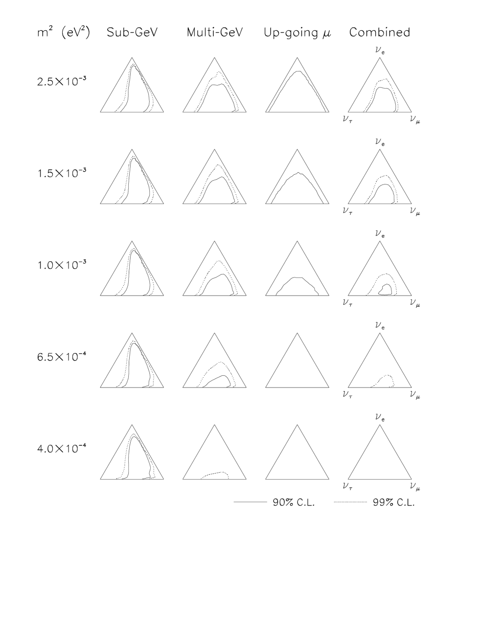
FIG. 15.: As in Fig. 14, but for different (lower) values of $m^{2}$.

D Fit to Super-Kamiokande and CHOOZ data

We combine SK and CHOOZ data (30+1 observables) through a joint $\chi^{2}$ analysis. The results are reported in Fig. 16.

Figure 16 shows the 90% and 99% C.L. in the triangle plot for selected values of $m^{2}$, ranging from $4\times 10^{-3}$ eV² (upper triangles) to $6.5\times 10^{-4}$ eV² (lower triangles). The left column of triangles reports the fit to SK data only (as derived from Figs. 14 and 15). The middle column reports the fit to CHOOZ data, which exclude a large horizontal stripe. In fact, the nonobservation of $\nu_{e}$ disappearance implies that $\nu_{3}$ is either very close to the upper corner $\nu_{e}$ (so as to suppress oscillations) or very close to the lower side ($\nu_{\mu}\leftrightarrow\nu_{\tau}$ oscillations being unobservables in CHOOZ). Clearly, the addition of the CHOOZ bounds to the SK fit (right column of triangles) cuts significantly the upper part of the solutions, so that only relatively low values of $U^{2}_{e3}$ are allowed. However, the CHOOZ bounds are rapidly weakened as $m^{2}$ is decreased, and for $m^{2}=1.5\times 10^{-3}$ eV² the parameter $U^{2}_{e3}$ can be as large as $\sim 0.15$ at 90% C.L. and $\sim 0.25$ at 99% C.L., corresponding to a significant $\nu_{e}$ appearance probability [see Eq. (8)]. Therefore, the CHOOZ data constrain but do not exclude the role of $\nu_{e}$ mixing and electron appearance in the interpretation of the SK data (see also [38, 83]). In particular, part of the electron excess in the SG and MG samples could be explained by nonzero values of $U^{2}_{e3}$ rather than by uncertainties in the overall neutrino flux normalization. Nonzero values of $U^{2}_{e3}$ also contribute to distort the zenith distributions [38], as discussed in Sec. V A.

So far we have seen the impact of CHOOZ on the mixing parameters $U^{2}_{\alpha 3}$. The impact on the square mass difference $m^{2}$ is summarized in Fig. 17, which shows the $\chi^{2}$ as a function of $m^{2}$, for unconstrained values of the mixing angles and for both fits to SK (dashed lines) and SK+CHOOZ (solid lines). The minimum value of $\chi^{2}$ is $28.3$ for SK and $29.8$ for SK+CHOOZ, indicating a good fit to the data (30 and 31 observables, respectively). The CHOOZ data help to constrain $m^{2}$ on the higher range, but its role decreases rapidly for $m^{2}\lesssim 10^{-3}$ eV².

Also shown in Fig. 17 are the 90% and 99% C.L. intervals for $m^{2}$, which allow values as low as $5\times 10^{-4}$ eV². The possibility of exploring such low values of $m^{2}$ should be seriously considered in long baseline experiments. An interesting result of Fig. 17 is the stability of the $m^{2}$ range indicated by SK—it does not change dramatically by adding the CHOOZ constraint. Therefore, the inclusion of the CHOOZ data in the global analysis affects more the mixing than the mass parameter.

A comparison of SK and pre-SK bounds is illuminating. Figure 17 should be compared with Fig. 10 of [36], where we combined the data from NUSEX, Fréjus, IMB, and Kamiokande (sub-GeV and multi-GeV) in a three-flavor analysis. The comparison shows that the SK and SK+CHOOZ bounds on $m^{2}$ are perfectly consistent with the pre-SK bounds. The SK+CHOOZ data appear to improve significantly the old upper bound on $m^{2}$, but give a lower bound very similar to the pre-SK data. Notice that we have long since claimed that the popular value $m^{2}\sim 10^{-2}$ eV² overestimated the best fit for pre-SK data, and that values as low as $5\times 10^{-4}$ eV² were compatible with the atmospheric $\nu$ data [36]. We plan to perform a joint analysis of all the data (SK+CHOOZ+pre-SK) in a future work.

VI Implications of the $3\nu$ analysis

In this Section we examine some implications of our three-flavor analysis for the phenomenology of atmospheric, long-baseline, and solar neutrino experiments, as well as for model building.

A Atmospheric $\nu$ phenomenology

The SK atmospheric data are consistent with $3\nu$ oscillations with dominant $\nu_{\mu}\leftrightarrow\nu_{\tau}$ transitions ($U^{2}_{\mu 3}\cdot U^{2}_{\tau 3}\gtrsim 0.2$ at 90% C.L.) and subdominant $\nu_{e}\leftrightarrow\nu_{\mu,\tau}$ mixing $(U^{2}_{e3}\lesssim 0.15)$. The mass square difference $m^{2}$ is favored in the range $\sim 0.8\times(10^{-3}$–$10^{-2})$ eV². Can one improve significantly such indications only with SK or other atmospheric data?

Large $\nu_{\mu}\leftrightarrow\nu_{\tau}$ mixing should generate a $\nu_{\tau}$ flux comparable to the $\nu_{\mu}$ flux at the detector site. However, the “contamination” of $\mu$-like and $e$-like events from $\tau$ production and subsequent leptonic decay is estimated to be very small in SK [4]. Therefore, there seems to be little hope to test the $\nu_{\mu}\leftrightarrow\nu_{\tau}$ channel through $\tau$ appearance in SK. Nevertheless, the possibility of enhancing (through appropriate cuts) the $\tau\to\mu$ and $\tau\to e$ “pollution” in selected $\mu$ and $e$ event samples may deserve further attention in other atmospheric $\nu$ detectors such as Soudan2.

The tests of $\nu_{e}$ mixing (i.e., of the matrix element $U^{2}_{e3}$) can certainly be improved with higher statistics SK data, in particular with more multi-GeV upgoing electron and muon events. Such data samples are characterized by a relatively high $\nu_{\mu}/\nu_{e}$ flux ratio (see Sec. II A), and thus are more sensitive to an increase of $e$-like events due to $\nu_{\mu}\leftrightarrow\nu_{e}$ transitions. Multi-GeV data are already more powerful than SG (and UP$\mu$) data in constraining $U^{2}_{e3}$ (see Fig. 15).

FIG. 16.: Three-flavor analysis in the triangle plot. Separate and combined fits to Super-Kamiokande and CHOOZ. The CHOOZ data exclude large horizontal stripes in the triangle plots. The combined SK+CHOOZ solutions are closer to pure $\nu_{\mu}\leftrightarrow\nu_{\tau}$ oscillations as compared with the fit to SK data only. However, the allowed values of $U^{2}_{e3}$ are never negligible, especially in the lower range of $m^{2}$.

FIG. 17.: Bounds on $m^{2}$ for unconstrained mixing, as derived from the $\chi^{2}$ analysis of SK data, with and without CHOOZ. The 90% and 99% C.L. intervals correspond to variations of $\chi^{2}-\chi^{2}_{\rm min}=6.25,\,11.36$ for three degrees of freedom (the oscillation parameters).

While the elements $U^{2}_{\alpha 3}$ determine the amplitude of oscillations, which can be already derived from total event rates, the parameter $m^{2}$ governs the phase of oscillations, and thus it can be derived only through event spectra. Hypothetical spectra of neutrino events as a function of $E_{\nu}$ and $L$ would be the most sensitive probes of $m^{2}$. Unfortunately, a complete kinematical closure of $\nu$-induced events cannot be achieved in SK, so neither $E_{\nu}$ nor $L$ can be precisely reconstructed, especially for low-energy events. This intrinsic feature will eventually limit the maximum accuracy of $m^{2}$ fits attainable with SK data only. In this respect, the possibility of improving the $E_{\nu}$ and $L$ reconstruction in experiments as Soudan2 [14] (through observation of the struck nucleon), or in high-density detectors as proposed in [84], appears extremely interesting and promising.

B Long Baseline experiments

Long baseline (LBL) accelerator experiments, such as K2K [29], MINOS [28], and various CERN-Gran Sasso proposals [30], are expected to confirm the atmospheric neutrino signal with a controlled beam. Since both two-flavor [4] and three-flavor analyses like ours show that $m^{2}$ can be as low as $\sim 5\times 10^{-4}$ (99% C.L.), the design of low-energy beams should be pursued seriously. If the atmospheric $m^{2}$ range can be covered completely, then it suffices to have either a $\nu_{\mu}$ disappearance or a $\nu_{\tau}$ appearance signal to confirm the SK anomaly.

However, we think that long baseline experiments should be designed to measure oscillation parameters, rather than merely to confirm an oscillation effect already found by SK. Measuring the oscillation parameters is a task that demands careful considerations, especially if $3\nu$ oscillations are to be tested (for $2\nu$ oscillations, see the lucid discussion in [85]).

The determination of $m^{2}$ requires energy spectra analyses, and thus high-statistics event samples. If $m^{2}$ happens to be in the low range of the experimental sensitivity, the $\tau$ appearance sample might consist of just a handful of events. The $e$ appearance event sample might also be small if $U^{2}_{e3}\to 0$. Therefore, a safe reconstruction of $m^{2}$ should be based mainly on $\mu$ event spectra from the $\nu_{\mu}\to\nu_{\mu}$ disappearance channel, where most of the signal is expected in any case. This implies a good monitoring of the initial $\nu_{\mu}$ beam with a near detector.

The determination of the matrix elements $U^{2}_{\alpha 3}$ requires that several oscillation channels are probed at the same time—redundancy is never enough to constrain neutrino mixing [40]. For instance, the $\nu_{\mu}\to\nu_{\mu}$ disappearance channel is sensitive only to $U^{2}_{\mu 3}$ but tells nothing on $U^{2}_{e3}$ or $U^{2}_{\tau 3}$, while the $\nu_{\mu}\to\nu_{\tau}$ appearance channel is sensitive to the product $U^{2}_{\mu 3}U^{2}_{\tau 3}$ but it cannot separate the two factors $U^{2}_{\mu 3}$ and $U^{2}_{\tau 3}$ nor measure $U^{2}_{e3}$ [see Eqs. (7,8)]. These aspects of $3\nu$ mixing tests [39, 40] in long-baseline experiments are better appreciated in Fig. 18.

Figure 18 shows, in the first column of triangles, the region allowed by SK+CHOOZ for selected values of $m^{2}$. The second column shows, superimposed, the prospective regions that can be probed at $\sim 90\%$ C.L. by K2K [29], both in the $\nu_{\mu}\to\nu_{\mu}$ channel (slanted bands) and in the $\nu_{\mu}\to\nu_{e}$ channel (hyperbola). It appears that K2K might not reach, in the $\nu_{\mu}\to\nu_{e}$ channel, sufficient sensitivity to probe the values of $U^{2}_{e3}$ allowed by SK+CHOOZ. The disappearance channel $\nu_{\mu}\to\nu_{\mu}$ can cover the whole SK+CHOOZ region, but only for $m^{2}\gtrsim 2\times 10^{-3}$ eV². Therefore, K2K is basically expected to give information on $U^{2}_{\mu 3}$ for $m^{2}\gtrsim 2\times 10^{-3}$ eV², given the sensitivities prospected in [29].

With respect to K2K, the MINOS experiment is being designed to probe lower values of $m^{2}$ and to explore also the $\nu_{\mu}\to\nu_{\tau}$ appearance channel (the region below the hyperbola touching the $\nu_{\mu}\to\nu_{\tau}$ side in Fig. 18). Possible signals in the three channels $\nu_{\mu}\to\nu_{e,\mu,\tau}$ will constrain the quantities $U^{2}_{\mu 3}U^{2}_{e3}$, $U^{2}_{\mu 3}$, and $U^{2}_{\mu 3}U^{2}_{\tau 3}$, respectively, so that the elements $U^{2}_{\alpha 3}$ can be pinpointed for $m^{2}\gtrsim 2\times 10^{-3}$ eV² if the uncertainties are kept small. For lower $m^{2}$’s, MINOS rapidly looses sensitivity in at least one of the oscillation channels, and it might be difficult to constrain the neutrino mixing parameters.

Notice that, for $U^{2}_{e3}\sim 0.15$ and the $U^{2}_{\mu 3}\sim 0.5$ (allowed by SK+CHOOZ), the $\nu_{\mu}\to\nu_{e}$ appearance probability is $P_{\mu e}=4U^{2}_{\mu 3}U^{2}_{e3}\langle S\rangle\sim 0.3\cdot\langle S\rangle$, where $\langle S\rangle(<1)$ is the oscillation factor in Eq. (9), averaged over the $\nu$ beam energy spectrum. Depending on $\langle S\rangle$ and on the specific mixing parameters, values of $P_{\mu e}$ as large as 15% appear possible in properly designed LBL experiments.

A final remark is in order. The sensitivity regions in Fig. 18 have been derived from the prospective estimates reported in the experiment proposals [29, 28], which are in continuous evolution (even more so for the CERN to Gran Sasso proposals [30], not shown). Therefore, the above considerations on K2K and MINOS are to be considered as preliminary and qualitative. Nevertheless, it remains true that LBL experiments might face some difficulties in constraining the $3\nu$ mixing parameters, especially if $m^{2}$ is low or if the three oscillation channels $\nu_{\mu}\to\nu_{e,\mu,\tau}$ cannot all be probed. Re-directing the goal of LBL experiments from “confirming the Super-Kamiokande signal” to “measuring the parameters $(m^{2},U^{2}_{e3},U^{2}_{\mu 3},U^{2}_{\tau 3})$” would be beneficial to the current debate on various LBL proposals.

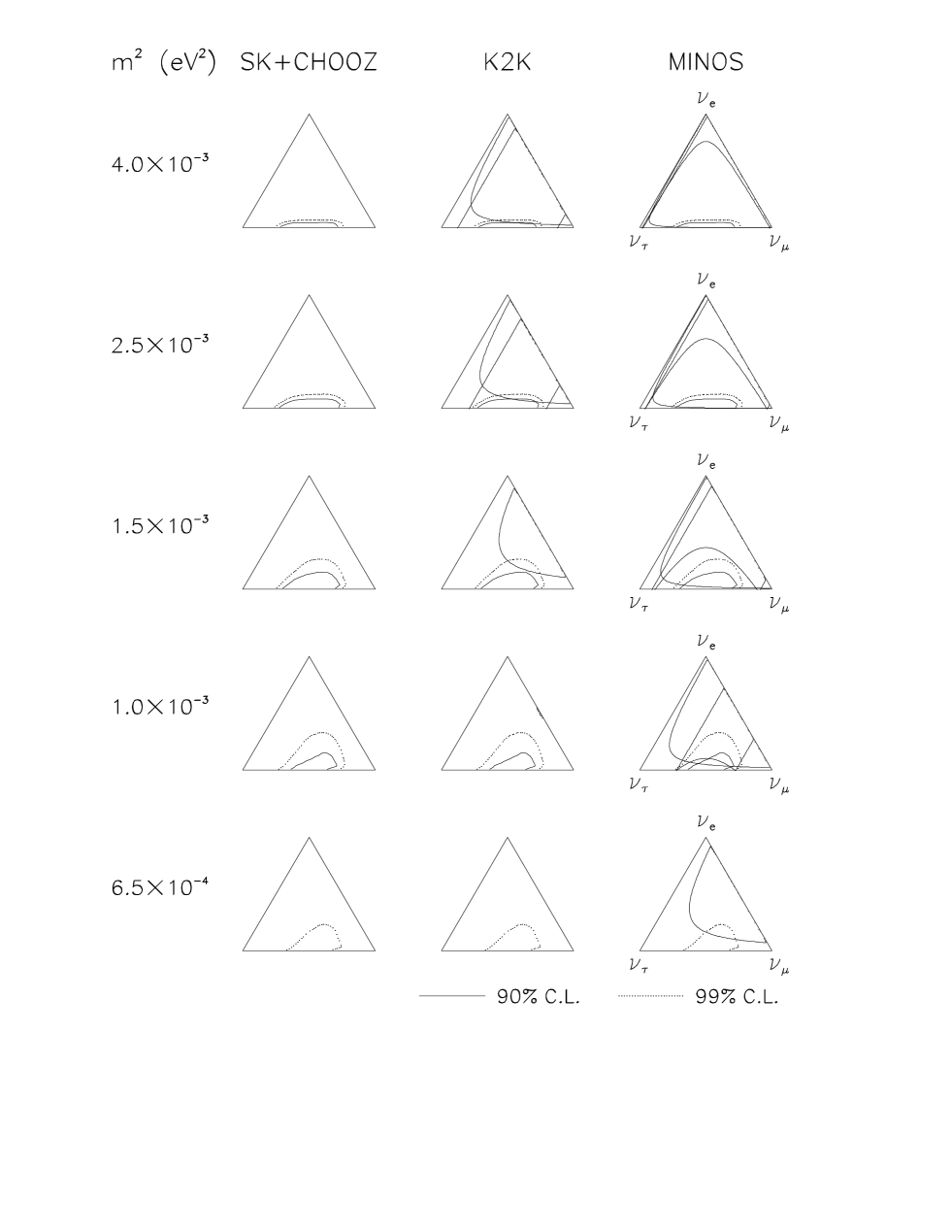
FIG. 18.: Regions of the SK+CHOOZ solutions explorable by two Long Baseline accelerator experiments (K2K and MINOS) through various oscillation channels. See the text for details.

FIG. 19.: Beyond the approximation of one mass scale dominance: example of effects induced by the subdominant mass scale $\delta m^{2}$, for oscillation parameters allowed by atmospheric, CHOOZ, and solar neutrino data.

C Solar neutrino problem

In the limit $\delta m^{2}\ll m^{2}$ [Eq. (4)], experiments with terrestrial (atmospheric, accelerator and reactor) neutrino beams probe the parameters $(m^{2},U^{2}_{e3},U^{2}_{\mu 3},U^{2}_{\tau 3})$. In the same approximation, solar neutrino experiments probe the parameters $(\delta m^{2},U^{2}_{e1},U^{2}_{e2},U^{2}_{e3})$, i.e., the small mass square difference and the mass composition of $\nu_{e}$ [32].

Therefore, both terrestrial and solar $\nu$ experiments probe the element $U^{2}_{e3}$, which parametrizes the mixing of $\nu_{e}$ with the “lone” neutrino mass eigenstate $\nu_{3}$. The effect of such mixing on solar neutrinos is to give an energy-independent contribution to the disappearance of $\nu_{e}$’s from the sun. Since this contribution is basically proportional to the square of $U^{2}_{e3}$ [32], sizable mixing is required to have large effects. However, as $U^{2}_{e3}$ is constrained by the SK+CHOOZ fit, such effects are relatively small to be detected in the current solar neutrino experiments. The smallness of $U^{2}_{e3}$ also reduces the “coupling” of the terrestrial and solar parameter spaces [72].

Nevertheless, it is interesting to notice that a preference for small values of $U^{2}_{e3}$ emerges naturally from solar neutrino data only, in both matter-enhanced [43, 32] and vacuum [86] three-flavor oscillation fits. An updated analysis using the latest SK solar neutrino data would be desirable to confirm such indication. In fact, a more pronounced preference of solar $\nu$’s for relatively small values of $U^{2}_{e3}$ would be a nontrivial, although indirect, hint that both solar and terrestrial $\nu$ data are consistent within the same $3\nu$ oscillation scenario.

The relation between solar and atmospheric neutrinos is not necessarily confined to a preference for relatively small values of the mixing matrix element $U^{2}_{e3}$. For instance, if the assumption in Eq. (4) is violated, atmospheric neutrinos can become sensitive to the subleading oscillations driven by $\delta m^{2}$, i.e., by the “solar neutrino” mass difference. Figure 19 shows a representative case beyond the $\delta m^{2}\ll m^{2}$ approximation. The values chosen for the oscillation parameters $(\delta m^{2},m^{2},\omega,\phi,\psi)$ are allowed at 99% C.L. by the present SK+CHOOZ bounds and by the pre-SK, three-flavor solar $\nu$ analysis in [32]. The effect of the subdominant mass scale $\delta m^{2}$ can be evaluated by comparing the solid curves ($\delta m^{2}=0$) and the dashed curves ($\delta m^{2}\neq 0$). Of course, the effect is more significant when $\delta m^{2}L/E_{\nu}$ is larger, i.e., for upgoing SG events, while it rapidly decreases at higher energies (MG and UP$\mu$ samples) and shorter pathlengths ($\cos\theta\to 1$). For SG$\mu$ events, however, the effect approaches the size of the error bars and thus it might be probed by SK! However, the strategies for disentangling the oscillations driven by $m^{2}$ and $\delta m^{2}$ are nontrivial and will be investigated in a future work.

D Models of neutrino mass and mixing

Theoretical or phenomenological models of neutrino mass and mixing try to predict, or “explain,” the set of parameters $(m_{1},m_{2},m_{3})$ and $U_{\alpha i}$. Our analysis constrains the subset of parameters $(m^{2},U^{2}_{\alpha 3})$, provided that $\delta m^{2}$ is sufficiently small ($\lesssim 10^{-4}$). Many models that try to explain solar+atmospheric $\nu$ data fall within this category, and are thus strongly constrained by the SK+CHOOZ bounds worked out in this paper. For instance, the so-called bimaximal mixing model [76], characterized by $(U^{2}_{e3},U^{2}_{\mu 3},U^{2}_{\tau 3})=(0,1/2,1/2)$ for atmospheric neutrinos [and by $(U^{2}_{e1},U^{2}_{e2},U^{2}_{e3})=(1/2,1/2,0)$ for solar neutrinos] is allowed for $m^{2}\gtrsim 10^{-3}$ eV² (see Fig. 15). Conversely, the trimaximal mixing model [87], characterized by $(U^{2}_{e3},U^{2}_{\mu 3},U^{2}_{\tau 3})=(1/3,1/3,1/3)$ for atmospheric neutrinos [and by $(U^{2}_{e1},U^{2}_{e2},U^{2}_{e3})=(1/3,1/3,1/3)$ for solar neutrinos] appears to be strongly disfavored by our combined SK+CHOOZ analysis (it would correspond to the center of each triangle in Figs. 14 and 15). Of course, many other models (see, e.g., the classification in [88]) can be tested through our bounds on the oscillation parameters, provided that the dominance of the mass scale $m^{2}$ is assumed for atmospheric neutrinos.

Other models try to explain the atmospheric anomaly and the LSND evidence [89] for $\nu_{\mu}\to\nu_{e}$ oscillations, with an allowance for an energy-averaged suppression of the solar neutrino flux. Arguments disfavoring such scenarios are discussed in [42] (see, in particular, Table VI of [42] and related comments). One such model has been recently proposed in [90], where $m^{2}\sim 0.4$ eV² is assumed to drive the oscillations in the LSND experiment [89] range, as well as energy-averaged oscillations of atmospheric $\nu$’s, while $\delta m^{2}\sim 10^{-4}$–$10^{-3}$ eV² is assumed to drive energy-dependent oscillations of atmospheric $\nu$’s. Both $\delta m^{2}$ and $m^{2}$ can then contribute to the solar neutrino deficit through energy-averaged oscillations. Since the bounds worked out in Sec. V D assume $\delta m^{2}\ll 10^{-4}$ eV², and thus do not apply to such model, we have performed a numerical analysis of SK data ad hoc, using the same mass-mixing parameters as in [90]. We find that the resulting zenith angle distributions of muons (not shown) are only mildly distorted, and that the model is disfavored by the SK atmospheric data at $>99\%$ C.L., with or without matter effects. We mention that, for the choice of parameters in [90], matter effects influence significantly the zenith distributions, making them flatter than in vacuum. The semi-quantitative calculations in [90] showed a more optimistic agreement to the SK data, in part because matter effects were ignored. In addition, the large value for $U^{2}_{\tau 3}$ chosen in [90] does not appear in agreement with the global analysis of laboratory neutrino oscillation searches (including the LSND data) performed in [91].

VII Summary and conclusions

We have performed a three-flavor analysis of the SK atmospheric neutrino data, in a framework characterized by the mass-mixing parameters $(m^{2},U^{2}_{e3},U^{2}_{\mu 3},U^{2}_{\tau 3})$, in the hypothesis of one mass scale dominance. The variations of the zenith distributions of $\nu$ events in the presence of flavor oscillations have been investigated in detail. Fits to the SK data, with and without the additional CHOOZ data, strongly constrain the parameter space. Detailed bounds have been shown in triangle graphs, embedding the unitarity condition $U^{2}_{e3}+U^{2}_{\mu 3}+U^{2}_{\tau 3}=1$. The allowed regions include the subcase $U^{2}_{e3}=0$, corresponding to pure $\nu_{\mu}\leftrightarrow\nu_{\tau}$ oscillations. However, values of $U^{2}_{e3}>0$ are also allowed. In particular, for $m^{2}$ close to (or slightly below) $10^{-3}$ eV², $U^{2}_{e3}$ can be as large as $\sim 0.15$ (at 90% C.L.). Scenarios with $U^{2}_{e3}>0$ correspond to genuine three-flavor oscillations and are characterized by a rich phenomenology, not only for atmospheric $\nu$’s, but also for solar and laboratory neutrino oscillation searches. In particular, challenging opportunities are disclosed for $\nu_{e}$ appearance searches in long baseline experiments. Our analysis also places strong constraints on models of neutrino mass and mixing. In addition, we have examined many facets of the SK data and of their interpretation, that will deserve further attention when the experimental and theoretical uncertainties will be reduced.

A Calculation of zenith distributions

The calculation of the zenith angle distributions of SG and MG lepton events involves the numerical evaluation of multiple integrals of the form

$$\Phi\otimes\sigma\otimes\varepsilon\otimes P\ ,$$ (A1)

where $\Phi$ is the unoscillated neutrino spectrum, $\sigma$ is the differential cross section for lepton production, $\varepsilon$ is the detector efficiency for lepton reconstruction, and $P$ is the oscillation probability [43, 36].

The efficiency function $\varepsilon$ is not always reported in the experimental papers. In particular, it has not been explicitly given by the SK Collaboration so far. We faced a similar problem in the analysis of the Kamiokande multi-GeV data performed in [36]. Our solution [36] was to use the energy distribution of the parent neutrinos $\nu$ that produce a detected lepton $\ell$, namely,

$$\frac{dN_{\nu}}{dE_{\nu}}=\frac{d\Phi_{\nu}}{dE_{\nu}}\int\!dE_{\ell}\,\frac{d\sigma_{\nu}}{dE_{\ell}}\,\varepsilon(E_{\ell})\ ,$$ (A2)

where $E_{\ell}$ is the lepton energy. This distribution, which gives information on the factor $\Phi\otimes\sigma\otimes\varepsilon$ in Eq. (A1), has been published in [8] for the Kamiokande experiment. Concerning SK, we have used the analogous information from [56].

Using the energy distribution of parent neutrinos, it is possible to reconstruct the zenith distribution of the final leptons, provided that the smearing induced by neutrino-lepton scattering angle is taken into account [36]. While for the old Kamiokande multi-GeV data we approximated this effect with an energy-independent smearing angle of $\sim 17^{\circ}$, for SK we properly take into account the distribution of the lepton scattering angle and its dependence on the energy, which is especially relevant for SG events [92]. We find good agreement with the SK estimate of the average scattering angle as a function of energy (as reported in [21], p. 99). Concerning the neutrino fluxes, we refer to [5] except for SG events, where we use the differential spectra from [6] with geomagnetic corrections [93].

Since the distributions of parent neutrinos in [56] are given in arbitrary units, we need to normalize the total area of our estimated SK lepton distributions (SG and MG, in the absence of oscillations) to the corresponding values simulated by the SK Collaboration, as reported in Table I (total rates). For SG events, this renormalization compensates, in part, for the fact that we use low-energy $\nu$ fluxes from [6, 93] instead than from [5]. Of course, a more direct calculation of the SG and MG distributions (avoiding the use of indirect information such as the parent $\nu$ distributions) is preferable; we intend to perform such calculation when the SK efficiency function $\varepsilon(E_{\ell})$ will be made publicly available. In any case, our present approach produces results in satisfactory agreement with SK zenith distributions for SG and MG events [18], as shown in Fig. 20. The small differences between our calculations and the SK simulations are not relevant, being comparable to the SK MonteCarlo statistical error.

Figure 20 also shows the UP$\mu$ distribution, for which we use a direct computation as in [37], with the following ingredients: GRV94 DIS structure functions [57], Lohmann et al. muon energy losses in the rock [59, 20], and the zenith dependence of the SK muon energy threshold from [19, 20]. Also for this distribution, we obtain a good agreement with the corresponding SK calculation (with the same inputs).

Notice that Fig. 20 refers to the no oscillation case. Some “oscillated” $\mu$-like and $e$-like event distributions (as well as their ratio $\mu/e$) have also been presented by the SK Collaboration in various Conferences, especially for the case of maximal $\nu_{\mu}\leftrightarrow\nu_{\tau}$ mixing. We obtain good agreement with SK also in such cases (not shown).

In conclusion, we are confident that our calculations of the zenith distributions represent a satisfactory approximation (not a substitute, of course) of the SK simulations. Improvements of our calculations for the SG amd MG samples are possible (with a more accurate knowledge of the SK detector efficiency) but do not appear to be decisive at present, in view of the good agreement reported in Fig. 20 and of the relatively large theoretical uncertainties discussed in the following Appendix.

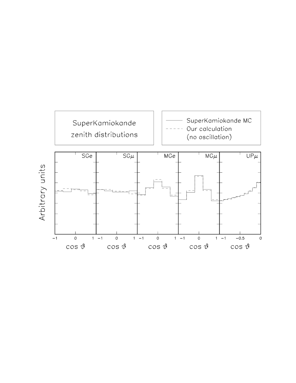
FIG. 20.: Angular distribution shape: comparison of the SK MonteCarlo simulations (solid lines) with our calculations (dashed lines).

B Statistical analysis

Fitting histograms is a delicate task. In general, the predictions in any two bins are correlated, and ignoring such correlations typically leads to significant variations in the allowed ranges for the fit parameters. Concerning the SK zenith distributions, this problem adds to the difficulty of evaluating the size of uncertainties associated to the theoretical neutrino flux calculations and to the neutrino cross section, as well as the variations of such uncertainties in terms of the neutrino energy and direction.

There is no easy solution to such problems, other than continually improving the calculations, understanding the role and the uncertainties of any input parameter, and removing as many approximations as possible [47, 48, 49]. Cosmic ray experiments can also help to constrain the models of atmospheric showers. The confidence in the estimated cross sections might benefit from a resurgence of experimental interest for low-energy neutrino interactions. In the meantime, it is wise to adopt conservative error estimates.

For each of the 30 SK zenith bins $\{b_{i}\}_{i=1,\dots,30}$ used in the analysis, we take the experimental statistical error $s_{i}$ from Tables I and II. The $30\times 30$ statistical error matrix $s^{2}_{ij}$ simply reads $s^{2}_{ij}=\delta_{ij}s_{i}s_{j}$. As a global systematic error $\sigma_{i}$ for each bin, we assume conservatively $\pm 30\%$ of the theoretical prediction (with or without oscillations). The systematic error matrix is then $\sigma^{2}_{ij}=\rho_{ij}\sigma_{i}\sigma_{j}$, where the correlation matrix $\rho_{ij}$ is evaluated as follows.

If the systematic uncertainties $\sigma_{i}$ had a single, common origin such as an overall normalization uncertainty, then the bin values $b_{i}$’s would be fully correlated ($\rho_{ij}=1$) and the systematics would cancel in any bin ratio $b_{i}/b_{j}$. However, the presence of several sources of uncertainties implies that $\rho_{ij}<1$ and that the ratio $b_{i}/b_{j}$ is affected by a residual uncertainty

$$\sigma^{2}(b_{i}/b_{j})=\sigma^{2}_{i}+\sigma^{2}_{j}-2\rho_{ij}\sigma_{i}\sigma_{j}\ ,$$ (B1)

where all $\sigma$’s represent fractional errors. For $\sigma_{i}=\sigma_{j}=\sigma(=0.3)$ the above relation can be inverted to give

$$\rho_{ij}=1-\frac{\sigma^{2}(b_{i}/b_{j})}{2\sigma^{2}}\ ,$$ (B2)

which allows to estimate $\rho_{ij}$ from the ratio error. For instance, if $b_{i}$ refers to downgoing SG $e$-like events and $b_{j}$ to the corresponding $\mu$-like events, with a $\mu/e$ uncertainty of, say, $\pm 5\%$, the corresponding correlation index is $\rho_{ij}=1-(0.05^{2})/(2\cdot 0.30^{2})=0.986$ [35].

The task is then reduced to the evaluation of the most important sources of errors for the ratios $b_{i}/b_{j}$. The total error for the $\mu/e$ flavor ratio (including the theoretical uncertainties and the experimental misidentification) is conservatively estimated to be $\pm 8\%$ for SG events and $\pm 12\%$ for MG events in [4]. For bins of equal flavor, one expects an additional energy-dependent uncertainty in the ratio $b_{i}/b_{j}$ due to uncertainties in the neutrino energy spectrum slope. In fact, by comparing the relative rates of SG, MG, and UP$\mu$ events calculated with different input fluxes (either [6] or [5]), we find typical ratio errors of $\pm 5\%$ for $b_{i}({\rm SG})/b_{j}({\rm MG})$ and $b_{i}({\rm MG})/b_{j}({\rm UP})$, and of $\pm 10\%$ for $b_{i}({\rm SG})/b_{j}({\rm UP})$, i.e., errors increasing with the relative difference between the mean energies of the event samples. Finally, one expects also angular-dependent errors for $b_{i}/b_{j}$, that we estimate to be at most $\pm 5\%$ when the difference between $|\cos\theta_{i}|$ and $|\cos\theta_{j}|$ is maximal (ratio of vertical to horizontal direction bins).

Qualitatively, all this means that the correlation between any two bins decreases from unity as the bins are more separated in energy, angle, and flavor, thus giving to the theoretical distributions some freedom to vary their shape. Quantitatively, we formalize the above estimates by generalizing Eq. (B2) as

$$\rho_{ij}=1-\frac{\sigma^{2}_{f}}{2\sigma^{2}}-\frac{\sigma^{2}_{E}}{2\sigma^{2}}-\frac{\sigma^{2}_{\theta}}{2\sigma^{2}}\ ,$$ (B3)

where $\sigma=30\%$, and: (i) $\sigma_{f}$ is the “flavor-dependent uncertainty,” equal to 10% for bins of different flavors and zero otherwise; (ii) $\sigma_{E}$ is the “energy-dependent uncertainty,” equal to zero for bins $(i,j)$ belonging to the same sample (SG, MG, or UP), to 5% for bins $(i,j)$ of the kind (SG,MG) or (MG,UP), and to 10% for bins $(i,j)$ of the kind (SG,UP); and (iii) $\sigma_{\theta}$ is the “direction-dependent uncertainty,” equal to $5\%$ times the difference between the mean direction cosines $|\langle\cos\theta\rangle_{i}|$ and $|\langle\cos\theta\rangle_{j}|$. For instance, the first bin of the SG$e$ distribution and the last bin of the UP$\mu$ distribution have the lowest correlation, $\rho_{ij}\simeq 0.874$, since they are the most distant in energy, flavor, and direction.

We finally define our $\chi^{2}$ function as

$$\chi^{2}=\sum_{ij}\Delta b_{i}\,(s^{2}_{ij}+\rho_{ij}\sigma_{i}\sigma_{j})^{-1}\,\Delta b_{j}\ ,$$ (B4)

where $\Delta b$ is the difference between the bin contents in Tables I and II and our theoretical calculations (with or without oscillations). We mention that the $\chi^{2}$ fit to the SK data appears to be rather sensitive to $\sigma_{f}$. Lowering its value from our present choice (10%, comparable to the estimates in Table II of [4]) to a few percent would shrink significantly the allowed regions but would also worsen the best fit. A reduction of this and other systematics would greatly improve the statistical power of oscillation hypothesis tests.

REFERENCES

- [1] Y. Totsuka for the Super-Kamiokande Collaboration, Lecture at 35th International School of Subnuclear Physics, Erice, Sicily, 1997, to appear in the Proceedings.
- [2] Super-Kamiokande Collaboration, Y. Fukuda et al., ICRR Report No. 411-98, hep-ex/9803006, to appear in Phys. Lett. B.
- [3] Super-Kamiokande Collaboration, Y. Fukuda et al., ICRR Report No. 418-98, hep-ex/9805006, submitted to Phys. Lett. B.
- [4] Super-Kamiokande Collaboration, Y. Fukuda et al., Boston University Report No. BU-98-17, hep-ex/9807003, submitted to Phys. Rev. Lett.
- [5] M. Honda, T. Kajita, K. Kasahara, and S. Midorikawa, Phys. Rev. D 52, 4985 (1995).
- [6] V. Agrawal, T.K. Gaisser, P. Lipari, and T. Stanev, Phys. Rev. D 53, 1314 (1996).
- [7] Kamiokande Collaboration, K. S. Hirata et al., Phys. Lett. B 205, 416 (1988); 280, 146 (1992).
- [8] Kamiokande Collaboration, Y. Fukuda et al., Phys. Lett. B 335, 237 (1994).
- [9] IMB Collaboration, D. Casper et al., Phys. Rev. Lett. 66, 2561 (1991); R. Becker-Szendy et al., Phys. Rev. D 46, 3270 (1992).
- [10] Soudan 2 Collaboration, W.W.M. Allison et al., Phys. Lett. B 391, 491 (1997). T. Kafka, in TAUP’97, Proceedings of the 5th International Conference on Topics in Astroparticle and Underground Physics (Gran Sasso, Italy, 1997), to appear in Nucl. Phys. B (Proc. Suppl.).
- [11] NUSEX Collaboration, M. Aglietta et al., Europhys. Lett. 8, 611 (1989).
- [12] Fréjus Collaboration, Ch. Berger et al., Phys. Lett. B 227, 489 (1989); 245, 305 (1990); K. Daum et al., Z. Phys. C 66, 417 (1995).
- [13] Kamiokande Collaboration, S. Hatakeyama et al., ICRR Report No. 421-98, hep-ex/9806038, submitted to Phys. Rev. Lett.
- [14] E. Peterson for the Soudan2 Collaboration, in Neutrino ’98 [18], to appear.
- [15] MACRO Collaboration, M. Ambrosio et al., Report INFN-AE-98-13, hep-ex/9807005; F. Ronga, in Neutrino ’98 [18].
- [16] Official page of Super-Kamiokande publications (papers, theses, notes, and proceedings), URL http://www-sk.icrr.u-tokyo.ac.jp/doc/sk/pub/ .
- [17] E. Kearns, in TAUP’97 [10], Report hep-ex/9803007.
- [18] T. Kajita, in Neutrino ’98, Proceedings of the XVIII International Conference on Neutrino Physics and Astrophysics, Takayama, Japan, June 1998, to appear. Transparencies available at the URL http://www-sk.icrr.u-tokyo.ac.jp/nu98/scan/ .
- [19] A. Habig, M. Takahata, and M. Yoshida for the Super-Kamiokande Collaboration, Poster presented at Neutrino ’98 [18], available at the URL http://hep.bu.edu/∼superk/upmu.html .
- [20] S. Hatakeyama, PhD thesis, Tohoku University, Feb. 1998, available at [16].
- [21] S. Kasuga, PhD thesis, University of Tokyo, Jan. 1998, available at [16].
- [22] J.W. Flanagan, PhD thesis, Hawaii University, Dec. 1997, available at [16].
- [23] Super-Kamiokande Collaboration, Y. Fukuda et al., ICRR Report No. 417-98, hep-ex/9805021, submitted to Phys. Rev. Lett.
- [24] CHOOZ Collaboration, M Apollonio et al., Phys. Lett. B 420, 397 (1998).
- [25] C. Bemporad for the CHOOZ Collaboration, in Neutrino ’98 [18], to appear.
- [26] A. Piepke for the Palo Verde Collaboration, in Neutrino ’98 [18], to appear.
- [27] F. Pietropaolo, in Neutrino ’98 [18], to appear.
- [28] MINOS Collaboration, “Neutrino Oscillation Physics at Fermilab: The NuMI-MINOS Project,” Report NuMI-L-375 (1998), available at the URL http://www.hep.anl.gov/NDK/Hypertext/numi_notes.html .
- [29] Y. Oyama for the K2K Collaboration, Proceedings of the YITP Workshop on Flavor Physics, Kyoto, Japan, 1998 (to appear), hep-ex/9803014.
- [30] G. Acquistapace et al., “The CERN Neutrino beam to Gran Sasso (NGS),” CERN Yellow Report 98-02, available at the URL http://preprints.cern.ch/cernrep/1998/1998.html .
- [31] Updated information on Long Baseline and other neutrino oscillation experiments can be found at the “Neutrino Oscillation Industry” URL http://www.hep.anl.gov/NDK/Hypertext/nuindustry.html .
- [32] G.L. Fogli, E. Lisi, and D. Montanino, Phys. Rev. D 54, 2048 (1996).
- [33] B. Faïd, G.L. Fogli, E. Lisi, and D. Montanino, University of Bari Report BARI-TH-299-98, hep-ph/9805298, to appear in Astropart. Phys.
- [34] G.L. Fogli, E. Lisi, and D. Montanino, University of Bari Report BARI-TH-296-98, hep-ph/9803309, to appear in Phys. Lett. B.
- [35] G.L. Fogli and E. Lisi, Phys. Rev. D 52, 2775 (1995).
- [36] G.L. Fogli, E. Lisi, D. Montanino, and G. Scioscia, Phys. Rev. D 55, 4358 (1997).
- [37] G.L. Fogli, E. Lisi, and A. Marrone, Phys. Rev. D 57, 5893 (1998).
- [38] G.L. Fogli, E. Lisi, A. Marrone, and D. Montanino, Phys. Lett. B 425, 421 (1998).
- [39] G.L. Fogli, E. Lisi, and G. Scioscia, Phys. Rev. D 52, 5334 (1995).
- [40] G.L. Fogli and E. Lisi, Phys. Rev. D 54, 3667 (1996).
- [41] E. Lisi, Proceedings of New Era in Neutrino Physics, a Satellite Symposium after Neutrino ’98 [18], Tokyo Metropolitan University, Tokyo, June 1998, to appear. Transparencies available at the URL http://musashi.phys.metro-u.ac.jp/neutrino.html .
- [42] G.L. Fogli, E. Lisi, D. Montanino, and G. Scioscia, Phys. Rev. D 56, 4365 (1997).
- [43] G.L. Fogli, E. Lisi, and D. Montanino, Phys. Rev. D 49, 3626 (1994).
- [44] G.L. Fogli, E. Lisi, and D. Montanino, Astropart. Phys. 4, 177 (1995).
- [45] Y. Oyama, Phys. Rev. D 57, 6594 (1998).
- [46] T.K. Gaisser, M. Honda, K. Kasahara, H. Lee, S. Midorikawa, V. Naumov, and T. Stanev, Phys. Rev. D 54, 5578 (1996).
- [47] T. K. Gaisser, in New Era in Neutrino Physics [41], to appear.
- [48] M. Honda, in New Era in Neutrino Physics [41], to appear.
- [49] G. Battistoni et al., “A new calculation of the atmospheric neutrino flux; The FLUKA approach,” in TAUP’97 [10], to appear.
- [50] T. Sanuki for the BESS Collaboration, in New Era in Neutrino Physics [41], to appear.
- [51] CAPRICE Collaboration, G. Barbiellini et al., Nucl. Instr. and Methods A371, 169 (1996); M. Boezio et al., Report INFN/AE-98/06, submitted to Astrophys. Journal.
- [52] MASS2 Collaboration, P. Papini et al., in ICRC’95, Proceedings of the 24th International Conference on Cosmic Rays, Rome, Italy, 1995, edited by H. Moraal, J.K. Gaisser, and J. Arafune (Arti Grafiche Editoriali, Urbino, 1995), Vol. 4, p. 1033; G. Basini et al., ibidem, Vol. 1, p. 585.
- [53] MASS2 Collaboration, G. Basini et al., in ICRC’97, Proceedings of the 25th International Conference on Cosmic Rays, Durban, South Africa, edited by M.S. Potgieter, B.C. Raubenheimer, and D.J. van der Walt (Potchefsroomse Universiteit, 1997), Vol. 6, p. 381.
- [54] F. Cafagna and M. Circella, private communication.
- [55] M. Circella, C.N. De Marzo, T.K. Gaisser, and T. Stanev, in ICRC’97 [53], Vol. 7, p. 117.
- [56] We thank Y. Totsuka for providing us with the energy spectra of parent neutrinos corresponding to simulated sub-GeV and multi-GeV muon and electron events.
- [57] M. Glück, E. Reya, and A. Vogt, Zeit. Phys. C 67, 433 (1995).
- [58] H. Plotow-Besch, “PDFLIB: The Parton Density Function Library,” User’s Manual, Version 7.09, available at the URL http://consult.cern.ch/writeup/pdflib .
- [59] W. Lohmann, R. Kopp, and R. Voss, CERN Yellow Report No. 85-03.
- [60] M.C. Gonzalez-Garcia, H. Nunokawa, O.L.G. Peres, T. Stanev, and J.W.F. Valle, Report hep-ph/9801368, to appear in Phys. Rev. D.
- [61] M.C. Gonzalez-Garcia, H. Nunokawa, O.L.G. Peres, and J.W.F. Valle, Report hep-ph/9807305.
- [62] P. Lipari and M. Lusignoli, Phys. Rev. D 57, 3842 (1998).
- [63] J.W. Flanagan, J.G. Learned, and S. Pakvasa, Phys. Rev. D 57, 2649 (1998).
- [64] R. Foot, R.R. Volkas, and O. Yasuda, Phys. Lett. B 421, 245 (1998).
- [65] O. Yasuda, Tokyo Metropolitan University Report TMUP-HEL-9805, hep-ph/9804400.
- [66] J.W. Flanagan, J.G. Learned, and S. Pakvasa, Hawaii Univ. report UH-511-901-98, hep-ph/9805343.
- [67] K.R.S. Balaji, G. Rajasekaran, and S. Uma Sankar, Report hep-ph/9806256.
- [68] F. Vissani and A.Yu. Smirnov, Report hep-ph/9710565.
- [69] L.J. Hall and H. Murayama, Univ. of California at Berkeley report No. UCB-PTH-98/31, hep-ph/9806218.
- [70] P. Lipari, T. Stanev, and T.K. Gaisser, Bartol Research Inst. Report BRI-98-13, astro-ph/9803093.
- [71] G. Feldman and R. Cousins, Phys. Rev. D 57, 3873 (1998).
- [72] M. Narayan, G. Rajasekaran, and S. Uma Sankar, Report hep-ph/9712409; C. Giunti, Report hep-ph/9802201.
- [73] R. Barbieri, L.J. Hall, D. Smith, A. Strumia, and N. Weiner, University of Pisa Report IFUP-TH-25-98, hep-ph/9807235.
- [74] V. Barger, T.J. Weiler, and K. Whisnant, Report hep-ph/9807319.
- [75] H. Minakata and O. Yasuda, Nucl. Phys. B 523, 597 (1998).
- [76] V. Barger, S. Pakvasa, T.J. Weiler, and K. Whisnant, Report hep-ph/9806387; A.J. Baltz, A.S. Goldhaber, and M. Goldhaber, Report hep-ph/9806540; M. Tanimoto, Report hep-ph/9807283.
- [77] Q.Y. Liu, S.P. Mikheyev, and A.Yu. Smirnov, ICTP Report IC-98-30, hep-ph/9803415.
- [78] P. Lipari and M. Lusignoli, Report hep-ph/9803440.
- [79] R. Foot, R.R. Volkas, and O. Yasuda, Phys. Rev. D 58, 013006 (1998).
- [80] D. Saltzberg, Phys. Lett. B 355, 499 (1995).
- [81] J.M. LoSecco, Reports No. hep-ph/9807359 and hep-ph/9807432.
- [82] C. Giunti, C.W. Kim, and M. Monteno, Nucl. Phys. B 521, 3 (1998).
- [83] R. Foot, R.R. Volkas, and O. Yasuda, Tokyo Metropolitan University Report TMUP-HEL-9803, hep-ph/9802287.
- [84] A. Curioni, G. Mannocchi, L. Periale, P. Picchi, F. Pietropaolo, and S. Ragazzi, Report hep-ph/9805249.
- [85] G. Battistoni and P. Lipari, Report hep-ph/9807475, to appear in the Proceedings of the 1998 Vulcano Workshop on Frontier Objects in Astrophysics and Particle Physics (Vulcano, Italy, 1998).
- [86] Z. Berezhiani and A. Rossi, Phys. Lett. B 219, 367 (1996); P. Osland and G. Vigdel, Report No. hep-ph/9806339.
- [87] P.F. Harrison, D.H. Perkins, and W.G. Scott, Phys. Lett. B 349, 137 (1995); 396, 186 (1997).
- [88] M. Tanimoto, Report hep-ph/9807517.
- [89] LSND Collaboration, C. Athanassopoulos et al., Phys. Rev. C 54 2685 (1996).
- [90] R.P. Thun and S. McKee, Report hep-ph/9806534.
- [91] G.L. Fogli, E. Lisi, and G. Scioscia, Phys. Rev. D 56, 3081 (1997).
- [92] T.K. Gaisser and J.S. O’Connell, Phys. Rev. D 34, 822 (1986).
- [93] T.K. Gaisser and T. Stanev, in ICRC’95, Proceedings of the 24th International Conference on Cosmic Rays, Rome, Italy, 1995, edited by H. Moraal, J.K. Gaisser, and J. Arafune (Arti Grafiche Editoriali, Urbino, 1995), Vol. 1, p. 694.