Comparisons of New Jet Clustering Algorithms for Hadron-Hadron Collisions

Abstract

We investigate a modification of the $k_{\perp}$-clustering jet algorithm for hadron-hadron collisions, analogous to the “Cambridge” algorithm recently proposed for $e^{+}e^{-}$ annihilation, in which pairs of objects that are close in angle are combined preferentially. This has the effect of building jets from the inside out, with the aim of reducing the amount of the underlying event incorporated into them. We also investigate a second modification that involves using a new separation measure. Monte Carlo studies suggest that the standard $k_{\perp}$ algorithm performs as well as either of these modified algorithms with respect to hadronization corrections and reconstruction of the mass of a Higgs boson decaying to $b\bar{b}$.

I Introduction

Jet-finding algorithms play a central role in the study of hadronic final states in all kinds of hard-scattering processes. Nowadays two types of jet algorithms are in common use: the so-called cone algorithms [1, 2] based ultimately on the Sterman-Weinberg [3] definition in terms of energy flow into an angular region, and the clustering algorithms [4, 5] in which jets are built up by iterative recombination. In $e^{+}e^{-}$ annihilation, the so-called Durham [6, 7, 8] version of the clustering algorithm has become most prevalent, although cone algorithms have also been applied [9, 10]. Up to now, cone algorithms have been more widely used in theoretical [11, 12, 13] and experimental [14, 15] studies of jets in hadron-hadron collisions. However, clustering algorithms have been proposed [16, 17, 18] and are beginning to be applied [19, 20] in this case also. Comparative theoretical studies [18, 21, 22, 23] have suggested that this would be beneficial, from the viewpoints of stability with respect to higher-order and non-perturbative corrections and improved mass resolution for heavy objects.

Recently, modifications to the Durham clustering algorithm for $e^{+}e^{-}$ final states have been proposed [24, 25] and some of their properties investigated [25, 26]. They mainly concern the two aspects of the algorithm which seem to be most open to improvement. The first concerns the order in which clustering occurs, and the second the resolution or separation measure that is used to decide whether clustering should occur. The general conclusion from $e^{+}e^{-}$ studies is that a change to angular ordering can help in the fine resolution of multi-jets and jet sub-structure, and that a smoother separation measure can reduce sensitivity to higher-order and non-perturbative effects.

In the present paper we investigate the effects of analogous modifications to the “standard” $k_{\perp}$-clustering algorithm [16, 17] for hadron-hadron collisions. We first review the criteria for a good jet algorithm, and then, after stating the standard algorithm and the proposed modifications precisely, we perform two types of comparative Monte Carlo studies.

For the first set of studies, in section V, we use a simple “tube” model [27, 28], representing the hadronic final state when no true jet production has occurred. Here the test of a good algorithm is the extent to which it can avoid generating spurious jets.

For the main investigations (section VI) we use the HERWIG [29] event generator to simulate true jet production over a range of transverse energies. We compare the jet properties at the parton and hadron (calorimeter) levels, as well as the sensitivity to the underlying soft event and calorimeter threshold. We also generate Higgs boson events and study the mass resolution for the decay $H^{0}\to b\bar{b}$.

Our conclusions are given in section VII.

II Criteria for a good jet-finding algorithm

Although a completely “correct” assignment of particles to jets is not a well-defined concept, owing to quantum interference effects, any jet algorithm must eventually assign all hadrons to a unique jet or the “underlying event” for the purpose of calculations. Clustering algorithms naturally assign particles unambiguously, while cone algorithms must add an ad hoc final step to deal with hadrons in overlapping cones. Association of particles that are close together in angle, or relative transverse momentum, is most natural from the viewpoint of QCD dynamics, and therefore the original JADE clustering criterion [5] based on invariant mass has been replaced by $k_{\perp}$-based criteria [4, 6] for the study of jets in $e^{+}e^{-}$ annihilation.

Identification of jets in hadron-hadron collisions is harder than in $e^{+}e^{-}$ annihilation. In the latter case, the beams are not made of composite particles, so the final states are cleaner. In particular, in a hadron-hadron collider, one must worry about “beam jets” and the “soft underlying event” (SUE), because the initial-state particles have quark constituents themselves. One expects the quarks not involved in hard scattering to continue along in a path near the beam line, possibly emitting some low-momentum particles at larger angles due to their soft interactions. The challenge is how to separate this “beam jet” and “underlying” hadronic energy from the products of the hard scattering process. For this purpose one needs an algorithm that eliminates particles with low transverse energy $E_{T}$ (relative to the beams) as early as possible from the clustering process, if they are not close to regions of high $E_{T}$ activity.

At the same time any jet-finding algorithm must possess certain basic properties in order to produce sensible (finite) results for quantities like jet cross sections. Included among these properties is insensitivity to low-energy gluon radiation (infrared safety). An algorithm is infrared safe if it does not distinguish between a state with an infinitely soft radiated gluon, and one without.

Also required is collinear safety. In the case of infrared safety, a zero energy emission can potentially lead to an infinite cross section. A parton emitted a zero angle can have the same effect. To prevent this blow-up in cross sections, the algorithm must not differentiate between two particles emitted along the same line. Now, it is clear that all algorithms will trivially satisfy these criteria at the calorimeter level, because the calorimeter will have finite resolution in energy and angle. However, one would hope to have an algorithm that possesses these good theoretical properties on its own.

In the case of hadron-hadron interactions, the jet algorithm must also allow for factorization of initial-state mass singularities. That is, it must allow the singularities due to initial-state collinear emissions to be factored out and replaced by non-perturbative parton distributions, leaving the hard scattering process to be calculated perturbatively.

Besides the above basic requirements, there are additional criteria one wishes to satisfy. A good jet-finding algorithm will find a minimum of “spurious jets”, that is, jets formed by combining unassociated soft particles from the underlying event or beam jets. All algorithms will eventually give rise to such jets, at sufficiently fine resolution. The level at which this begins to happen, and the fashion in which the spurious jets form, is of interest.

From an experimentalist’s viewpoint, an extremely important feature for an algorithm is its ability to reconstruct the momenta of the parent particles of the jets as accurately as possible, for example in the hadronic decays of heavy particles (top quarks, vector bosons, Higgs bosons, etc.). This is an invaluable tool in new particle searches, for establishing a potentially small signal on a potentially large background.

Other criteria for comparison include the shifts in the values of quantities that take place between the parton and hadron level. It is desirable to minimize these “hadronization corrections”.

In this paper, we compare spurious jet formation, hadronization effects, the ability to pick jets out of the underlying event, and the reconstruction of invariant masses, for the standard $k_{\perp}$-clustering algorithm and two possible variants of it.

III Algorithm definitions

We give here the precise definition of the standard $k_{\perp}$-clustering algorithm [16, 17] and then the proposed new variants. The choice of variables and combination procedure differ somewhat from those used for $e^{+}e^{-}$ physics. This is primarily because the hard parton scattering process has an unknown longitudinal boost in hadron-hadron collisions. One therefore needs to use variables that are approximately invariant under such boosts.

First we require some general definitions, as follows:

• Define a dimensionless cone size parameter $R$ (usually $R\leq 1$).

• For each object $i$ (hadron, calorimeter cell or whatever) in the final state, define the azimuthal angle $\phi_{i}$, the pseudorapidity

  $$\eta_{i}=-\ln\tan\left(\frac{\theta_{i}}{2}\right)$$ (1)

  and the transverse energy

  $$E_{Ti}=E_{i}\sin\theta_{i}$$ (2)

  where $\theta_{i}$ is the polar angle with respect to the direction of one of the incoming beams in the overall c.m. frame.

• The separation from the beams of object $i$ is

  $$d_{i}=E_{Ti}R\;.$$ (3)

• For each pair of objects $i$ and $j$ the angle is

  $$R_{ij}=\sqrt{(\eta_{i}-\eta_{j})^{2}+(\phi_{i}-\phi_{j})^{2}}$$ (4)

  and the separation is

  $$d_{ij}=\min\{E_{Ti},E_{Tj}\}R_{ij}\;.$$ (5)

• The combination procedure $i+j\to(ij)$ is

  $$E_{Tij} = E_{Ti}+E_{Tj}$$ (6)

  $$\eta_{ij} = \frac{(E_{Ti}\eta_{i}+E_{Tj}\eta_{j})}{E_{Tij}}$$ (7)

  $$\phi_{ij} = \frac{(E_{Ti}\phi_{i}+E_{Tj}\phi_{j})}{E_{Tij}}$$ (8)

A Standard $k_{\perp}$ algorithm

We use here the algorithm proposed in ref. [16] with the modifications suggested in ref. [17].

1. Find the pair $I$ and $J$ with $d_{IJ}=\min\{d_{ij}\}$.

   To determine whether clustering occurs, we compare this separation with the separation of the object “nearest” the beam.

2. Find the object $K$ with $d_{K}=\min\{d_{i}\}$.

3. If $d_{IJ}\leq d_{K}$ then combine $I+J\to(IJ)$, update the lists of $d_{ij}$’s and $d_{i}$’s accordingly, and go to 1.

4. If $d_{IJ}>d_{K}$ then store $K$ as a completed jet, remove it from the lists of $d_{ij}$’s and $d_{i}$’s, and go to 1.

5. Iterate until all jets are completed.

The presence of the cone size $R$ in Eq. (3) ensures that objects cannot be clustered unless their separation is less than $R$, since otherwise either $d_{I}$ or $d_{J}$ is less than $d_{IJ}$ and step four removes one of them.

Step four is also roughly akin to the “soft-freezing” that is used in the recently proposed Cambridge $e^{+}e^{-}$ algorithm [24]. By removing the less energetic objects from the list as clustering occurs, we prevent them from attracting additional partners that could build spurious jets.

B Proposed improved algorithm: $AO_{1}$

The $AO_{1}$ algorithm is an angular-ordered version of the standard algorithm. The basic idea of an angular-ordered algorithm is to use the angular variable $R_{ij}$, instead of the separation $d_{ij}$, to choose the pair of objects to be considered first for clustering.

1. Find the pair $I$ and $J$ with $R_{IJ}=\min\{R_{ij}\}$.

2. Find the object $K$ with $d_{K}=\min\{d_{i}\}$.

3. If $d_{IJ}\leq d_{K}$ then combine $I+J\to(IJ)$, update the lists of $R_{ij}$’s and $d_{i}$’s accordingly, and go to 1.

4. If $d_{IJ}>d_{K}$, then we must check whether the particle pair still remains within the angular cone size, $R$. If it does ($R_{IJ}\leq R$), then move to the pair $I^{\prime}$ and $J^{\prime}$ with the next-smallest value of $R_{ij}$ and repeat step 3, with $I^{\prime}$ and $J^{\prime}$ in place of $I$ and $J$.

5. If the particle pair does not lie within the fixed cone size ($R_{IJ}>R$) then store $K$ as a completed jet, remove it from the lists of $R_{ij}$’s and $d_{i}$’s, and go to 1.

6. Iterate until all jets are completed.

C Angular-ordered algorithm with new separation measure: $AO_{2}$

For the second angular-ordered algorithm we use the same steps as in $AO_{1}$ but change the definition of the separation measure between any two objects to

$$d_{ij}^{\prime}=\frac{2E_{Ti}E_{Tj}}{(E_{Ti}+E_{Tj})}R_{ij}\geq d_{ij}\;.$$ (9)

The separation between an object and the beam remains as before

$$d_{i}^{\prime}=E_{Ti}R=d_{i}\;.$$ (10)

This $d_{ij}^{\prime}$ measure has interesting properties. It retains the same basic shape as the original definition of $d_{ij}$, but it is now a smoothly varying function. This is shown in figure 1. It is analogous to the LUCLUS separation measure [4] used in $e^{+}e^{-}$ physics, where it has been found to have good features [25].

IV Theoretical properties of algorithms

It is immediately clear that all the above algorithms satisfy the infrared safety criterion. Recall that infrared safety is obtained if measured jet variables are unchanged when an $E_{T}\to 0$ parton is emitted. From the definition of $d_{ij}$ (or $d_{ij}^{\prime}$), it is clear that the proposed algorithms will immediately combine such a gluon with the hard parton that emitted it.

Similarly, it is clear that the algorithms are collinear safe. If a parton emits another parton along the same direction, the algorithms will immediately combine the two. Therefore, there will be no difference in the observable quantities in the case of collinear emission.

The algorithms also allow factorization of initial state singularities. As $\theta_{i}\to 0$, the separation from the beam, $d_{i}\to 0$. Therefore, the beam jets do not affect the combination of other jets, as hadrons collinear to the beams are immediately classified as completed jets by the algorithm, and taken off the combination list. This allows the remaining hadrons to go about combination unhindered.

Angular-ordered algorithms attempt more possible clusterings than the standard algorithm, because they may consider other pairs of objects before coming to the pair with the smallest separation under the $d_{ij}$ metric. However, any tendency towards over-clustering is balanced by the fact that the algorithms tend to start at the middle of each jet. As a consequence, we would hope that they tend to pick up fewer unassociated particles on the periphery of the jet. A rough schematic of such a case is shown in figure 2. In the standard algorithm, the two low-energy particles may combine. Then because the axis of the two has been pulled toward the centre, this composite jet may combine with the third particle. In the angular-ordered case, the jet is built up from the centre. Thus, the two central particles can combine, leaving the wide-angle particle to be resolved separately.

Cases such as these would lead us to hope that the angular-ordered algorithms might be able to separate the interesting high-$E_{T}$ jets more effectively from the soft underlying event. However, the above schematic only works in a fairly limited kinematic window. In most cases, the wide-angle radiation will still lie within the cone size $R$, and combination will still take place as in the standard $k_{\perp}$-algorithm.

V Tube model studies

Here a “tube” of particles is taken to be a cylinder of particles uniformly distributed in $\phi$ and $\eta$. The transverse momenta of the particles in the tube have a strongly damped exponential distribution. This simulates the hadronization of a soft hadronic collision or underlying event. There are no true jets, so any jet found is spurious, which is a useful comparative test of algorithms [24].

The particle multiplicity in this model is given by

$$\langle n\rangle=2\frac{\mu}{\langle p_{t}\rangle}\log\left(\frac{E_{\mbox{CM}}}{\mu}\right)$$ (11)

where $\mu$ is the invariant mass per unit rapidity (here set to 0.5 GeV), $E_{\mbox{CM}}$ is the centre-of-mass energy, and $\langle p_{t}\rangle$ gives the average transverse momentum per particle (again set to 0.5 GeV). The model was run at centre-of-mass energy 1 TeV, which gave $\langle n\rangle\simeq 15$ particles per event. Each algorithm was run on 10,000 events.

It was found that there was no difference in jet formation between the standard $k_{\perp}$ algorithm and the $AO_{1}$ algorithm. We looked at the number of particles included in the jet with the maximum $E_{T}$ (see table I). It is expected that the number of particles in this jet would be indicative of the amount of clustering that is done by the algorithm, as it is likely that if particles were combined, they would combine into a jet with a higher $E_{T}$ than that of a single particle.

We notice a striking similarity of $AO_{1}$ to the standard $k_{\perp}$-clustering algorithm by examining the energy spectra of the maximum $E_{T}$ jets (see figure 3). If additional spurious jet formation occurred in either case, one would expect to find that energy spectra to be broader and shifted to a higher energy. However, this signature is clearly absent, and the spectra are identical.

On the other hand, there is indeed a difference between the standard $k_{\perp}$ algorithm and the $AO_{2}$ algorithm (figure 4). Less clustering occurs in the case of the $AO_{2}$ algorithm. This is a result of the definition of the separation measure, $d_{ij}^{\prime}$. Notice that in figure 1 the separation measure used in $AO_{2}$ is greater than that for $AO_{1}$, for all values of $E_{T}$. As a result, the clustering condition will be satisfied less frequently. Consequently, the energy spectrum for the new separation measure $d_{ij}^{\prime}$ is shifted to lower energies, indicative of less clustering.

It is interesting to vary the cone size parameter, $R$, to see where a comparable amount of clustering occurs. As seen in figure 5, it is found that this happens when $R$ is increased from unity to a value of approximately $R=1.3$.

VI HERWIG Monte Carlo studies

HERWIG [29] is a Monte Carlo event generator that can be used to simulate many kinds of events. First the hard scattering process is calculated perturbatively, and then parton showers are generated until a given scale is reached, on the order of the hadron masses. Hadronization is simulated by combining partons into colorless clusters, which decay to hadrons. The model conserves local flavour and energy momentum flow. The underlying event is modelled as a separate collision between colorless clusters containing hadron remnants. For our study, QCD events were generated in symmetric $p\overline{p}$ collisions at a centre-of-mass energy of 1.8 TeV, as at Tevatron Run I.

For each type of test conducted, we attempted to ascertain the difference between applying a jet algorithm at the parton and calorimeter level. In order to run the algorithms at the parton level, the HERWIG simulation was simply stopped before hadronization, and the clustering was conducted on the partons at this stage. This is not entirely equivalent to the calculation of quantities via perturbation theory, but should still give a good comparative indication of hadronization effects. At the calorimeter level, a simple segmentation simulation was used [30]. The calorimeter was segmented into 63 equal cells in $\phi$, for a resolution of $.1$ radians and 100 cells in pseudo-rapidity covering a region from $-5\leq\eta\leq 5$, for the same rapidity resolution. The energy resolution of each cell is given by:

$$\frac{\sigma(E)}{E}=\frac{{\tt RES}}{\sqrt{E}}$$ (12)

where RES is a constant that differs for the hadronic and electromagnetic calorimeters. As a rough guide, we used ${\tt RES}=0.1$ for the electromagnetic and ${\tt RES}=0.5$ for the hadronic calorimeters ($E$ being measured in GeV).

To cover a range of jet energies, we varied the HERWIG parameter PTMIN, which sets the minimum parton transverse energy for the hard scattering processes. By varying this parameter, we examined jet transverse energies from 30 to 90 GeV with comparable statistics. A thousand events were collected at each value of PTMIN.

A Shift in jet axis

For each algorithm, we investigate the shift in jet axis, $\Delta R$, given by:

$$\Delta R=\sqrt{(\eta_{\mbox{parton}}-\eta_{\mbox{calorimeter}})^{2}+(\phi_{\mbox{parton}}-\phi_{\mbox{calorimeter}})^{2}}$$ (13)

This measure gives an indication of whether the algorithm is doing a good job of preserving the direction of parton energy flow at the calorimeter level. Depending on how invariant masses are reconstructed, this can have a radical effect on the masses of reconstructed particles.

Comparisons of the shift in the jet axis between parton level and calorimeter level show little difference between the algorithms. The scheme used to pair the calorimeter jets with parton jets was rudimentary. It simply took the two highest-$E_{T}$ jets and matched them in such a way as to minimize the total $\Delta R$ for these two jets. Other schemes are possible, such as optimizing over a larger number of jets, or looking for the highest-$E_{T}$ jets on opposite sides in azimuth. Variations of the $\Delta R$ matching scheme are a possible topic for future investigation. As shown in table II, the values of $\Delta R$ agree within statistical error. This is a somewhat surprising result, given the angular nature of the new algorithm.

Note also that the calorimeter has finite angular resolution, $\Delta R\simeq 0.1$. This serves to increase the value of $\Delta R$ for each algorithm, but should not affect any one more than the others. It seems, then, that all three algorithms that were investigated have similar shifts in jet axes.

B Jet radial moment

We also examine the change in the jet radial moment, which is a measure of how the energy is distributed about the jet axis. The radial moment is defined as [13, 23]:

$$\langle R\rangle=\sum_{\mbox{constituents}}\frac{E_{Ti}R_{i}}{E_{\mbox{jet}}}$$ (14)

where $R_{i}$ is the angular separation of the $i$th parton or calorimeter cell from the jet axis. A more compact jet, with its energy concentrated near the jet axis, has a smaller value of $\langle R\rangle$.

In a comparison between the radial moments, as defined in equation (14), it seems that all of the algorithms have similar discrepancies between the parton and calorimeter levels (see figure 7). However, note that the radial moment for the $AO_{2}$ algorithm is smaller. Again, this more collimated jet is a result of the larger separation measure (see figure 6).

As a consequence of these results on the radial moment, one would expect that the standard $k_{\perp}$-clustering algorithm and the $AO_{1}$ algorithm would perform similarly in the reconstruction of Higgs masses, while $AO_{2}$ would, in general, reconstruct lower masses. In section VI F, we find that the algorithms do, in fact, follow this behaviour.

C Jet energy spectra

The single jet inclusive transverse energy spectra were also examined for each of the algorithms. If more combination of particles took place for a given algorithm, one would expect to see a rise in cross section for higher jet energies, and a corresponding decrease for lower jet energies.

The spectra for the three algorithms are shown in figure 8. The standard $k_{\perp}$ algorithm and the $AO_{1}$ are quite similar to one another. Moreover, the results at the calorimeter and parton level are similar. This indicates relatively small hadronization corrections. Note, however, that both algorithms show a tendency to push the calorimeter spectrum to lower energies. This is most likely a consequence of forming spurious low-energy jets.

The spectrum shows an overall shift to lower energies in the case of the $AO_{2}$ algorithm. This is expected on account of the lower effective jet radius $R$ (see section V). It also seems to show slightly less distortion of the spectrum between the parton and the calorimeter levels.

D Sensitivity to calorimeter threshold energy

It was also investigated whether the two algorithms differed in their sensitivity to the threshold energy in the calorimeter cells. In the radial moment analysis (section VI B) only cells having energies greater than 1 GeV were included as initial “particles” for the algorithms to cluster.

This reduces the multiplicity of final-state particles to a reasonable number, thereby speeding up computing. The threshold value was changed from 1 GeV to 0.5 GeV, and 1000 events were generated at a minimum hard process scale (PTMIN) of 50 GeV.

Indeed all algorithms did show some sensitivity to the threshold. As expected, the radial moment increased at the smaller threshold. This corresponds to an increased number of calorimeter cells in the jet. However, the $AO_{1}$ algorithm and the standard $k_{\perp}$-clustering algorithm seem to be equally sensitive to the change in threshold energy, as shown in figure 9. The $AO_{2}$ algorithm seems to be slightly less sensitive to variation in the calorimeter threshold (figure 9).

All three algorithms displayed similar behaviour with respect to changes in shifts in the jet axis when the threshold was varied. This is illustrated in table III. All three algorithms seem to perform in an identical manner in this test case.

E Sensitivity to soft underlying events (SUE)

Because of an angular-ordered algorithm’s tendency to incorporate fewer particles at wide angles to the jet, one would hope that it would be less sensitive to the soft underlying events (SUE).

In HERWIG, one can turn the underlying event on and off with a simple switch. Runs were made with and without the SUE at a lower PTMIN=10 GeV. With the minimum hard scattering scale at a lower energy, one would expect the algorithms to have a difficult time separating the high-$E_{T}$ jets from the SUE. Indeed, we find the hadronization effects for all algorithms are worse with the SUE. However, the algorithms seem to display nearly identical reactions to the presence of a SUE. We find that the hadronization corrections are not reduced for either angular-ordered algorithm (figures 11 and 12).

F Reconstruction of Higgs mass

We also used HERWIG to generate Monte Carlo events containing a Standard Model Higgs boson with a mass of 110 GeV. At this mass, the Higgs boson decays almost entirely through the channel

$$H^{0}\to b\overline{b}$$ (15)

Events were generated in symmetric $p\overline{p}$ collisions at a centre-of-mass energy of 2 TeV, similar to the energy at Tevatron Run II.

In order to reconstruct the Higgs mass, one must select the two jets from which the Higgs boson will be reconstructed. We reconstructed the Higgs mass at the calorimeter level by simply looking at the invariant mass of the two most energetic jets. In an actual experiment, $b$ vertexing information could be taken into account to help pick the correct jets. Our method of jet selection is too simplistic, but it should be sufficient for comparative purposes.

The first feature to notice is that all the algorithms reconstruct the Higgs mass with a large width. The natural width of the Higgs boson at this energy is about 50 MeV, whereas the spread in the reconstructed mass is on the order of 30 GeV.

In the case of a calorimeter threshold of 1 GeV, every algorithm examined tends to undershoot the Higgs mass. This is partially due to resolving part of the $b$-jets into separate jets, which are not included in the final mass. In addition, energy can be lost to calorimeter cells that do not reach the threshold. Therefore, one would expect that the reconstructed mass would depend on the calorimeter threshold.

Initially, we used a rather harsh threshold of 1 GeV to limit the multiplicity of calorimeter cells in the final state. This slightly simplified situation is sufficient to show that the $AO_{1}$ algorithm and standard $k_{\perp}$ algorithm reconstruct Higgs masses in a nearly identical fashion, as illustrated in figure 13.

In order to reduce the energy lost through the high calorimeter threshold, we also examined the case where the threshold was lowered to an energy of 0.5 GeV, which practically eliminated the large mass offset.

As one would expect, there is a larger difference between the standard $k_{\perp}$ algorithm and the $AO_{2}$ algorithm. The Higgs mass reconstructed by the $AO_{2}$ algorithm with a cone size parameter $R=1$ is significantly below the mass reconstructed by the standard algorithm. Again, this is due to the fact that combination is suppressed by the lower effective cone size (see section V).

Recall that at $R=1.3$, the amount of clustering by the $AO_{2}$ algorithm was nearly equal to the amount of clustering with the standard $k_{\perp}$ algorithm. So it is of interest to see if the $AO_{2}$ algorithm reproduces results similar to the standard $k_{\perp}$ algorithm at this value of $R$. In fact, it does very nearly reproduce these results, as shown in figure 13. A summary of the reconstructed Higgs masses is given in table V. A simliar study using the cone algorithm yielded comparable results.

VII Conclusions

We have studied two possible modifications to the “standard” [16, 17] $k_{\perp}$-clustering algorithm for hadron-hadron collisions, both involving angular ordering, which has been found beneficial for some purposes in $e^{+}e^{-}$ jet studies [24, 25]. The first modified algorithm, $AO_{1}$, simply changes the order of clustering by examining the smallest-angle pair of remaining objects first. The second, $AO_{2}$, uses in addition a smoother measure of separation, analogous to that in the LUCLUS algorithm [4], which has also been recommended for $e^{+}e^{-}$ physics [25].

We find that, in contrast to the $e^{+}e^{-}$ case, these modifications do not appear to provide any significant advantage over the standard hadronic $k_{\perp}$-clustering algorithm. No significant difference was detected in the energy spectra, radial moment, or jet axes between the standard algorithm and the $AO_{1}$ algorithm. The new separation measure in the $AO_{2}$ algorithm did provide some differences. However, these differences could mostly be removed by simply increasing the cone size parameter, $R$. The $AO_{2}$ algorithm may have less sensitivity to the calorimeter threshold and the soft underlying event, but the differences are not very significant.

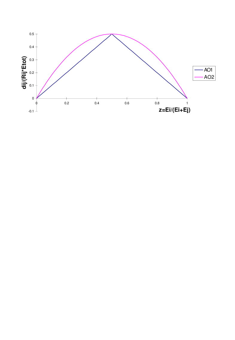
FIG. 1.: A comparison of different separation measures. We fix the total energy $E_{TOT}=E_{i}+E_{j}$ and vary $z=\frac{E_{i}}{E_{i}+E_{j}}$ from 0 to 1.

FIG. 2.: A misclustering of jets by the standard $k_{\perp}$-clustering algorithm.

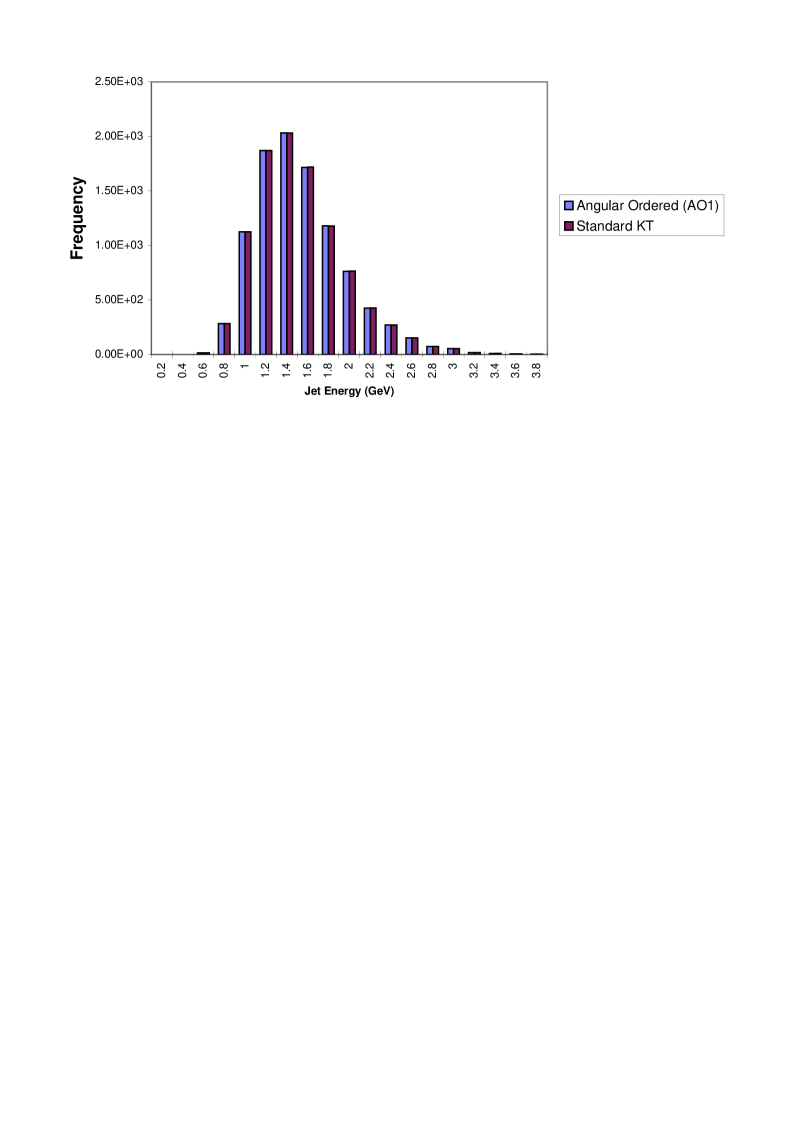
FIG. 3.: $E_{T}$ spectra of maximum $E_{T}$ jet in the tube model.

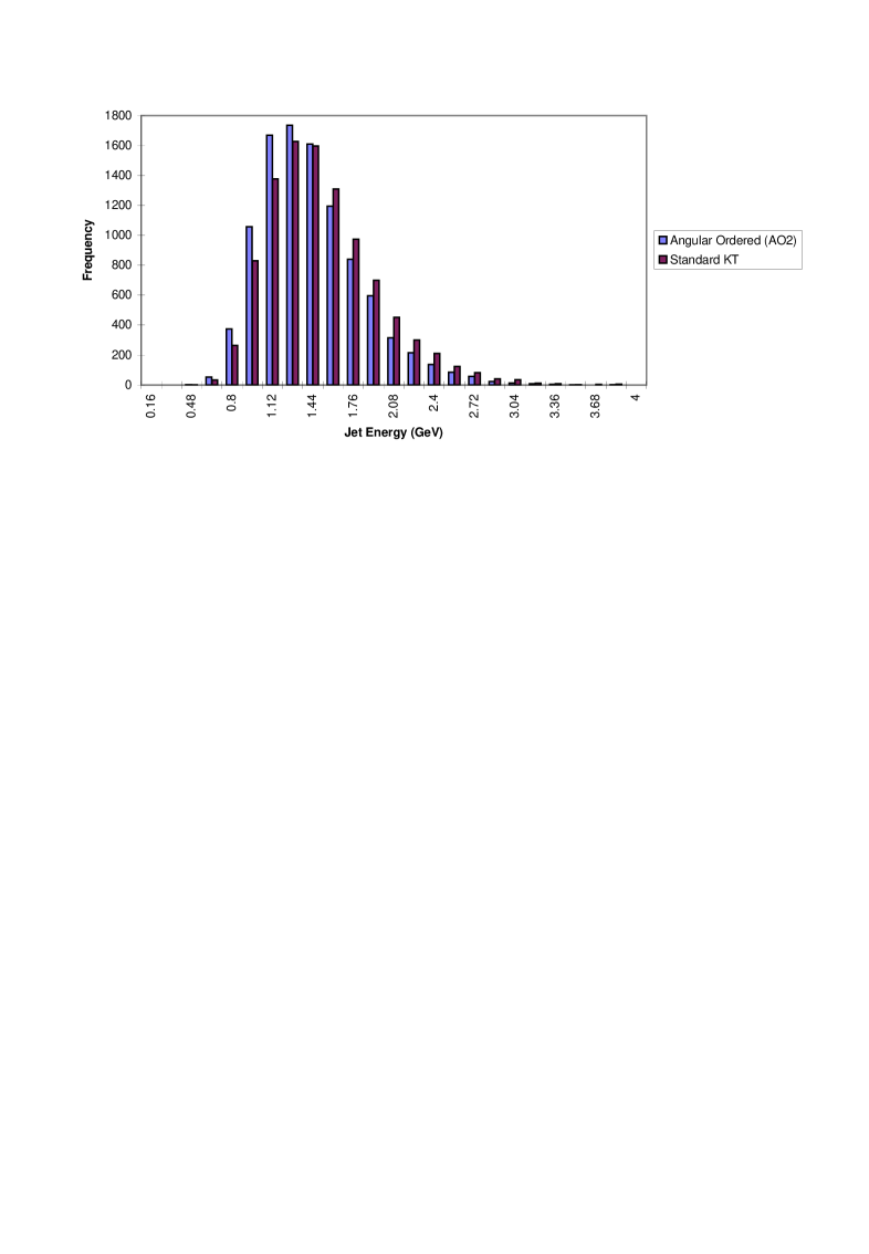
FIG. 4.: $E_{T}$ spectra of maximum $E_{T}$ jet in the tube model.

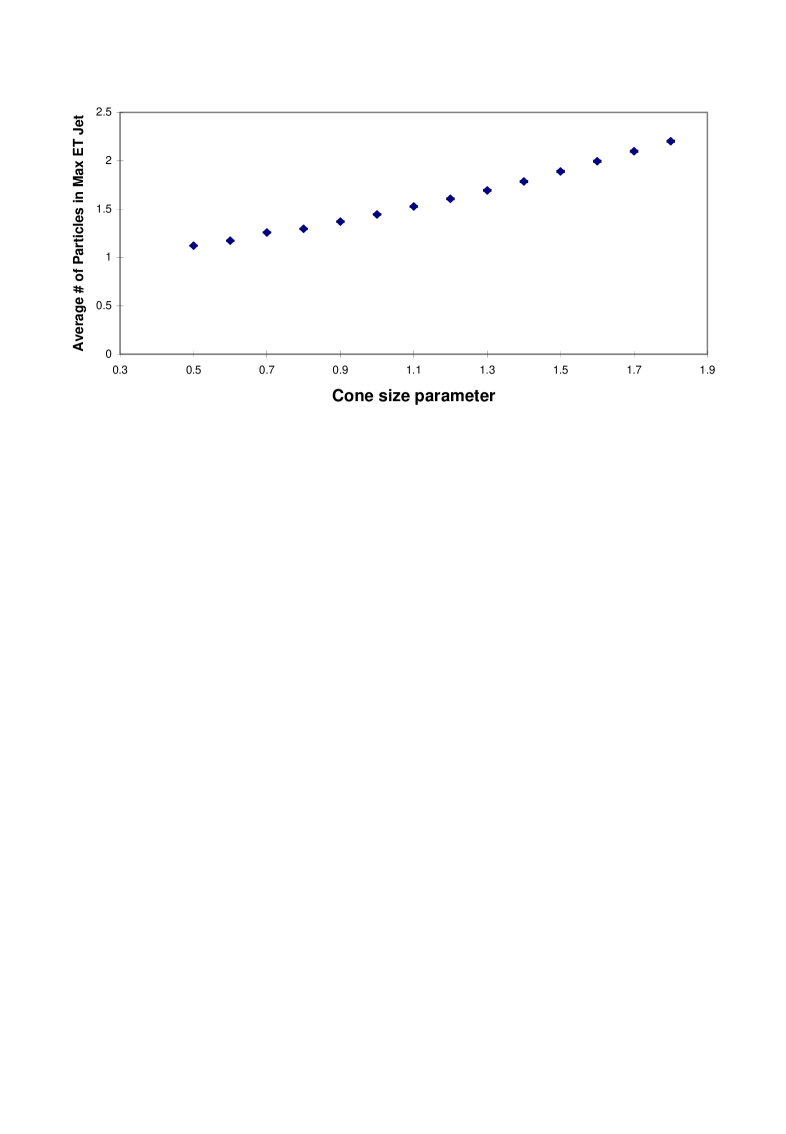
FIG. 5.: A measure of the amount of clustering done by the $AO_{2}$ algorithm as the cone size parameter is varied.

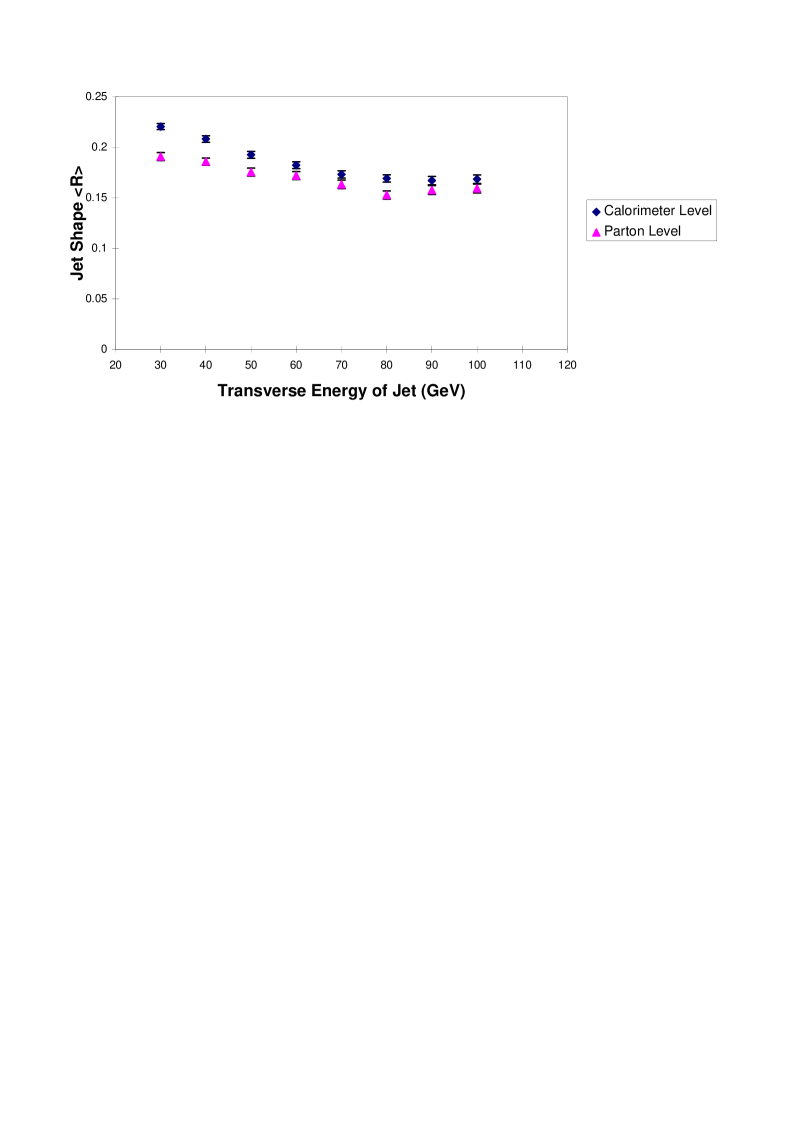
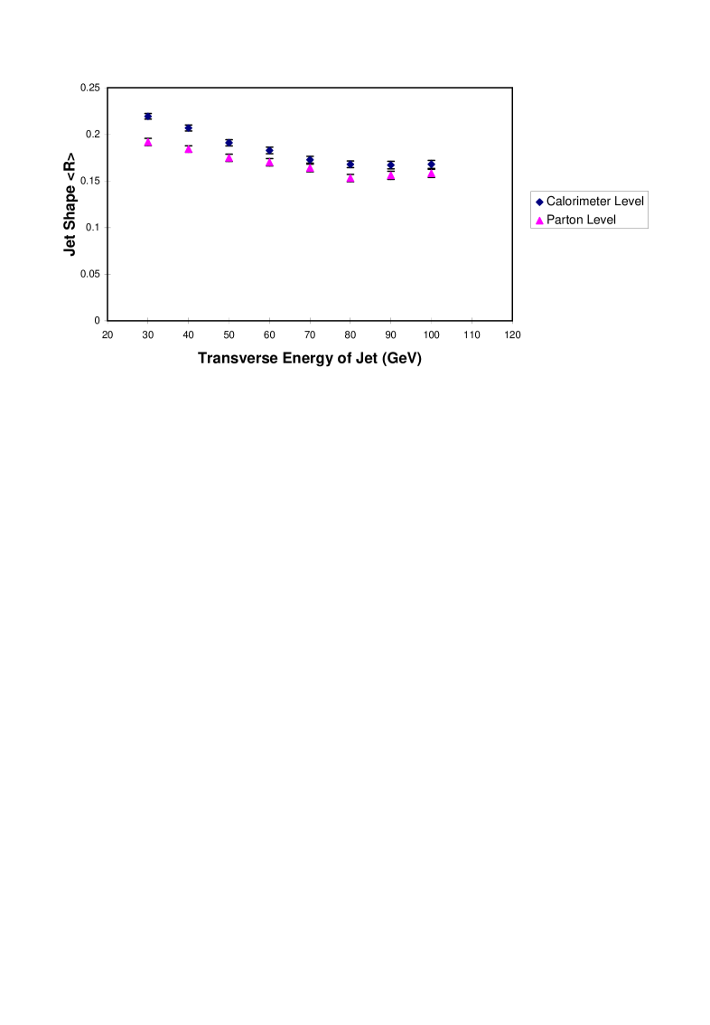
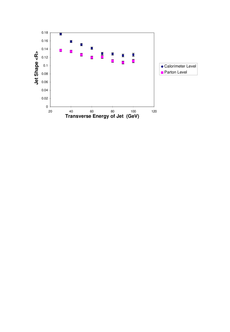
FIG. 6.: Radial moment curves for (a) Standard $k_{\perp}$, (b) $AO_{1}$ and (c) $AO_{2}$. The curves are constructed from 1000 events at each of PTMIN=30,50,70,90.

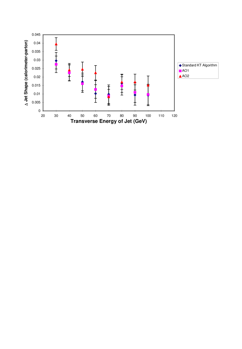
FIG. 7.: Difference between the calculated jet shapes at the parton and calorimeter level for each of the three algorithms under investigation. Each curve here is obtained by taking the difference between the two curves in each of the figures in figure 6.

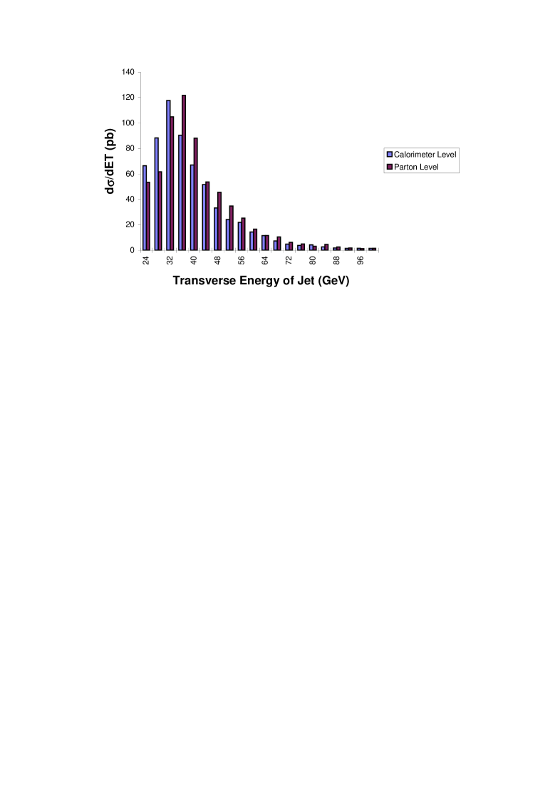
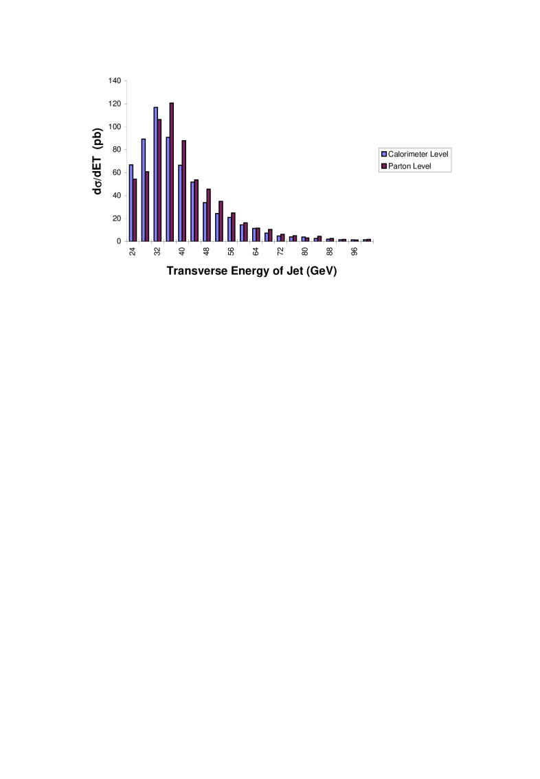
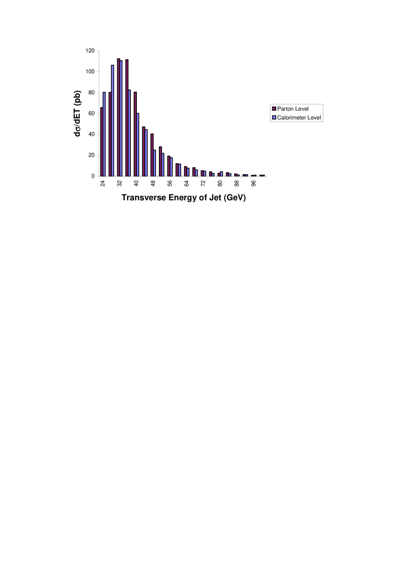
FIG. 8.: Transverse energy spectra of (a) Standard $k_{\perp}$, (b) $AO_{1}$, and (c) $AO_{2}$.

FIG. 9.: A comparison between the standard $k_{\perp}$ and $AO_{1}$ algorithms at different calorimeter thresholds. Here we examine the difference in the radial moment between the calorimeter and the parton levels.

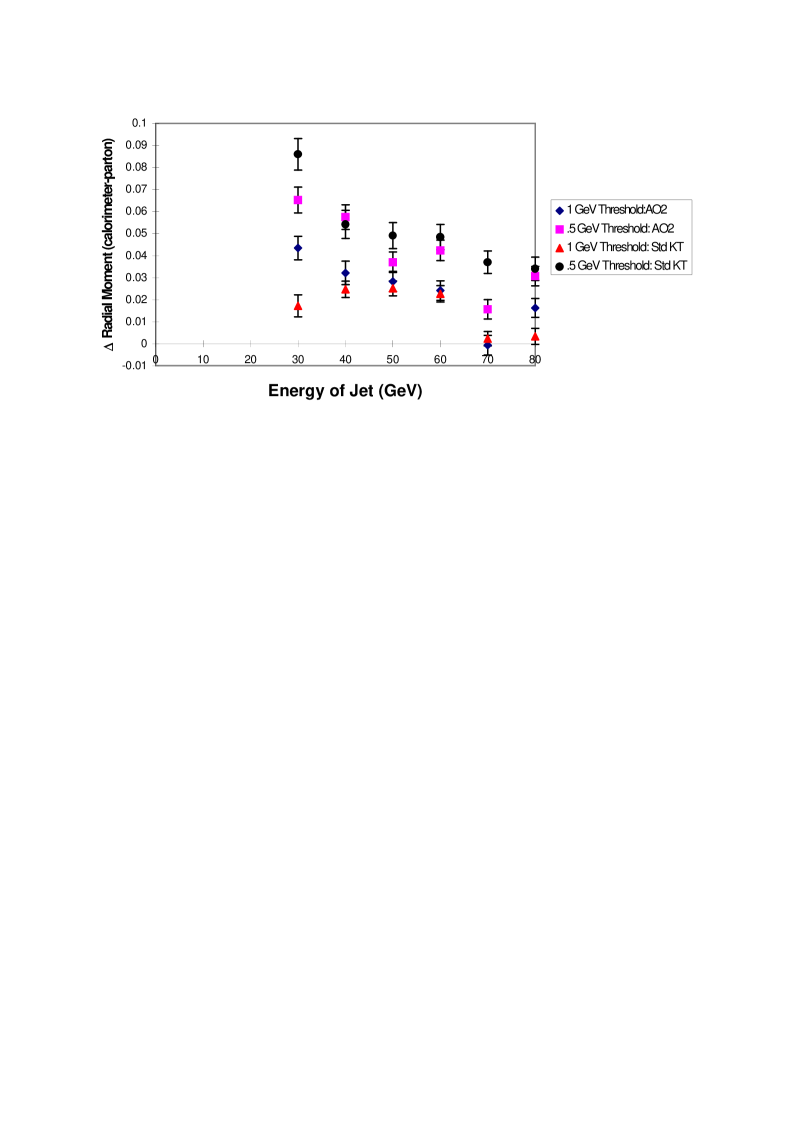
FIG. 10.: A comparison between the standard $k_{\perp}$ and $AO_{2}$ algorithms at different calorimeter thresholds. Here we examine the difference in the radial moment between the calorimeter and parton levels.

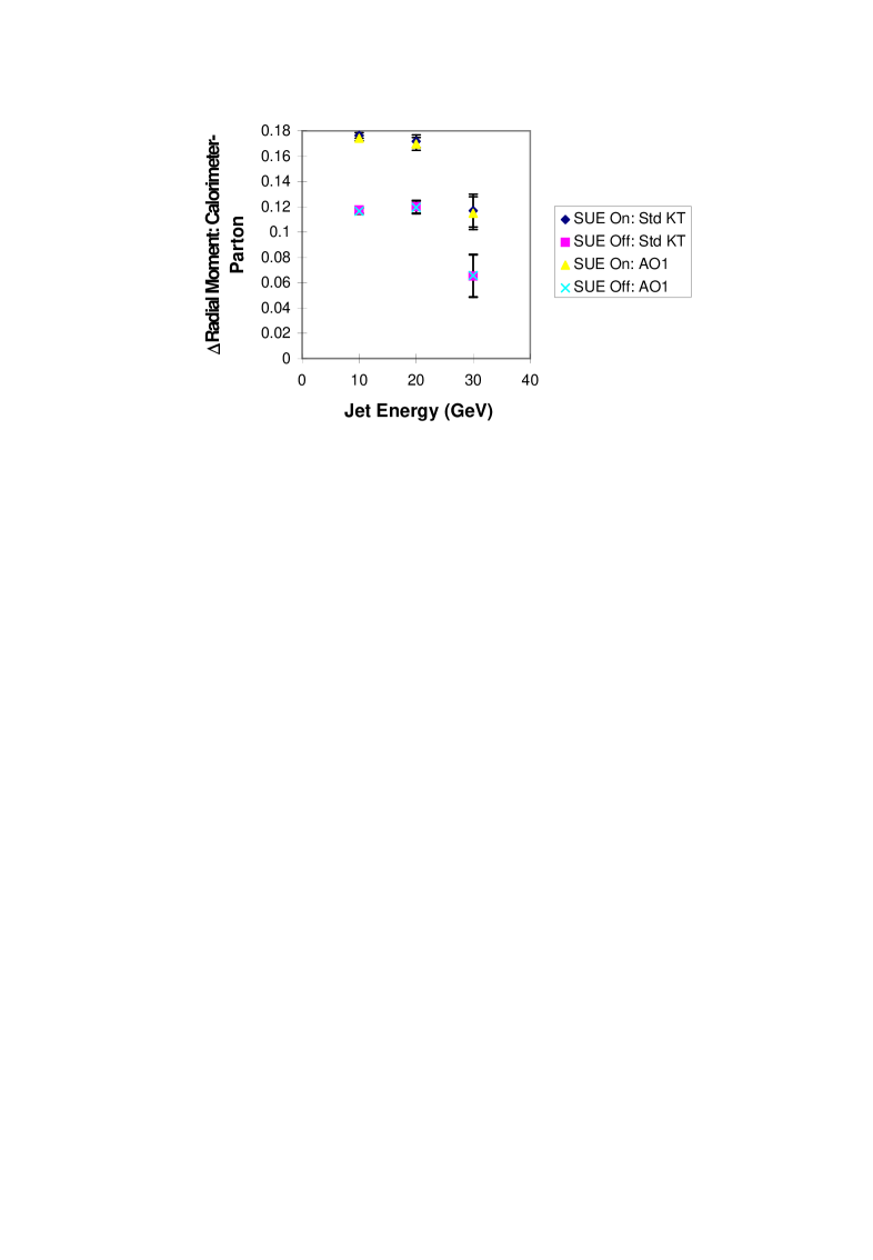
FIG. 11.: A comparison between the standard $k_{\perp}$ and $AO_{1}$ algorithms with and without soft underlying events. The plot is generated from 1000 events at a minimum hard scattering energy (PTMIN) of 10 GeV. The calorimeter threshold energy is 0.4 GeV.

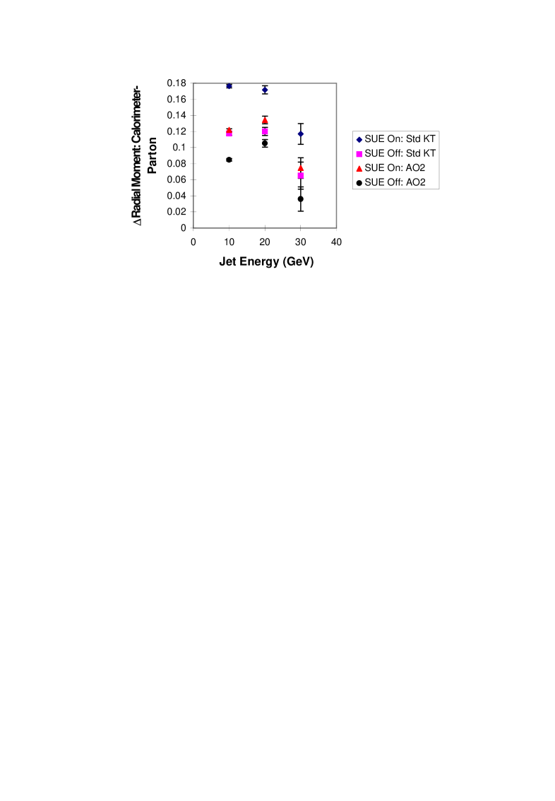
FIG. 12.: A comparison between the standard $k_{\perp}$ and $AO_{2}$ algorithms with and without soft underlying events. The plot is generated from 1000 events at a minimum hard scattering energy (PTMIN) of 10 GeV. The calorimeter threshold energy is 0.4 GeV.

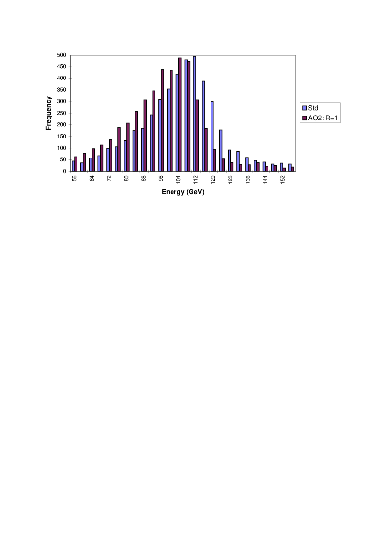
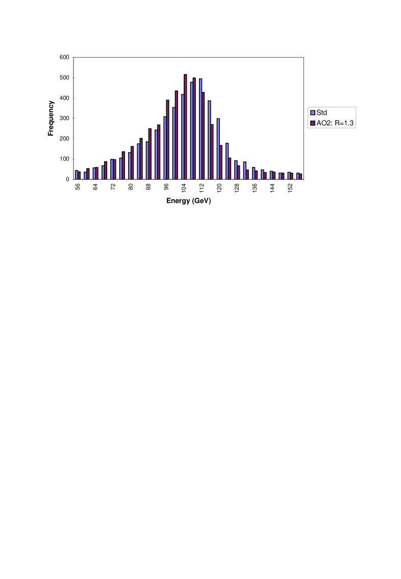
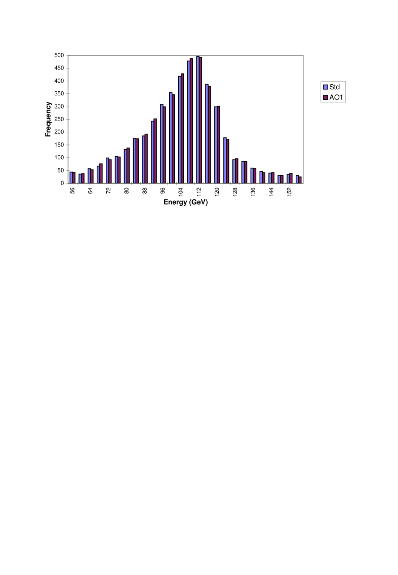
FIG. 13.: Higgs masses were reconstructed through 5000 Higgs decays generated by HERWIG. The calorimeter threshold is 0.5 GeV.

TABLE I.: Multiplicity of jets in a simple tube model. Errors are statistical.

Algorithm Type	Particles in Max $E_{T}$ jet
STANDARD $k_{\perp}$	$1.726\pm.007$
$AO_{1}$	$1.727\pm.007$
$AO_{2}$	$1.446\pm.006$

TABLE II.: Shift in Jet Axes. Errors are statistical. Here calorimeter threshold=1GeV.

PTMIN	Std. $k_{\perp}$ $\Delta R$	$AO_{1}$ $\Delta R$	$AO_{2}$ $\Delta R$
30	$.109\pm.008$	$.110\pm.008$	$.108\pm.009$
50	$.070\pm.006$	$.071\pm.005$	$.073\pm.006$
70	$.062\pm.005$	$.062\pm.005$	$.055\pm.005$
90	$.052\pm.004$	$.054\pm.005$	$.050\pm.005$

TABLE III.: Shift in Jet Axes. Errors are statistical. Here PTMIN is fixed at 50 GeV, and the sample size is 1000 events.

threshold	Std. $k_{\perp}$ $\Delta R$	$AO_{1}$ $\Delta R$	$AO_{2}$ $\Delta R$
.5 GeV	$.070\pm.006$	$.071\pm.005$	$.072\pm.006$
1 GeV	$.072\pm.005$	$.070\pm.005$	$.071\pm.006$

TABLE IV.: An analysis of the sensitivity of the shift jet axis to the underlying event. Errors are statistical. Here PTMIN is fixed at 10 GeV, and the calorimeter threshold is 0.4 GeV

SUE status	Std. $k_{\perp}$ $\Delta R$	$AO_{1}$ $\Delta R$	$AO_{2}$ $\Delta R$
ON	$.383\pm.019$	$.395\pm.020$	$.401\pm.020$
OFF	$.344\pm.019$	$.336\pm.018$	$.347\pm.019$

TABLE V.: Reconstructed Higgs mass. Statistical errors only (sample size 5000 events).

Threshold = 1 GeV
Algorithm Type	Mean Higgs Mass
$STANDARD$ $k_{\perp}$	$101.1\pm.6$
$AO_{1}$,	$101.0\pm.6$
$AO_{2}$, $R=1.3$	$98.9\pm.6$
$AO_{2}$, $R=1.0$	$95.1\pm.6$
Threshold = 0.5 GeV
Algorithm Type	Mean Higgs Mass
$STANDARD$ $k_{\perp}$	$110.7\pm.7$
$AO_{1}$,	$110.6\pm.7$
$AO_{2}$, $R=1.3$	$107.0\pm.6$
$AO_{2}$, $R=1.0$	$101.1\pm.6$