Periodic Euclidean Solutions of $SU(2)$-Higgs Theory

Abstract

We examine periodic, spherically symmetric, classical solutions of $SU(2)$-Higgs theory in four-dimensional Euclidean space. Classical perturbation theory is used to construct periodic time-dependent solutions in the neighborhood of the static sphaleron. The behavior of the action, as a function of period, changes character depending on the value of the Higgs mass. The required pattern of bifurcations of solutions as a function of Higgs mass is examined, and implications for the temperature dependence of the baryon number violation rate in the Standard Model are discussed.

I Introduction

Non-perturbative processes in quantum field theory such as tunneling, decay of metastable states, and anomalous particle production, are intimately connected with the existence and properties of non-trivial solutions of the associated classical field equations. In electroweak theory, baryon number violating processes are a consequence of topological transitions in which there is an order one change in the Chern-Simons number of the $SU(2)$ gauge field. At zero temperature, such transitions are quantum tunneling events, and the rate of these transitions is directly related to the classical action of instanton solutions of $SU(2)$ gauge theory [1]. At sufficiently high temperatures, the dominant mechanism for baryon number violation involves classical thermally activated transitions over the potential energy barrier separating inequivalent vacuum states. The configuration characterizing the top of the barrier is the static sphaleron solution of $SU(2)$-Higgs theory [2]; the energy of this solution controls the thermally-activated transition rate [3, 4].

As briefly reviewed below, when one lowers the temperature from the sphaleron dominated regime, the topological transition rate is related to the action of periodic classical solutions of the Euclidean field equations with a period $\beta$ equal to the inverse temperature. Very little detailed information is known, however, about the properties of periodic classical solutions in electroweak theory.

In this paper, we examine periodic solutions in $SU(2)$-Higgs theory (which represents the bosonic sector of electroweak theory in the limit of vanishing weak mixing angle). We focus exclusively on classical solutions which are real in Euclidean space. Classical perturbation theory is used to construct periodic time-dependent solutions in the neighborhood of the static sphaleron. The variation in the period as one changes the amplitude of oscillation away from the sphaleron (or equivalently the turning point energy of the solution) is found to change sign depending on the value of the Higgs mass. Unlike the situation in many simpler models, there is no periodic classical solution which smoothly interpolates between instantons at low temperature (long period) and the sphaleron at high temperature (short period). We argue that, depending on the value of the Higgs mass, one or two different branches of periodic solutions must exist, connected at a bifurcation point. The topological transition rate (in the semi-classical approximation) must show a “kink” as the temperature varies between zero and the electroweak transition temperature.

The non-existence of arbitrarily long period instanton-antiinstanton solutions in $SU(2)$-Higgs theory, and the consequent necessity for abrupt changes in the topological transition rate, has been previously noted [5, 6]. This phenomenon also occurs in two-dimensional $O(3)$ non-linear sigma models with soft symmetry breaking terms, which mimic many features of $SU(2)$-Higgs theory. Periodic classical solutions in softly-broken $O(3)$ sigma models have been studied in detail by several authors [5, 6]. We will argue that the behavior of periodic solutions found in the sigma model mimics the situation in $SU(2)$-Higgs theory when the Higgs mass is sufficiently small, but that for larger Higgs mass an additional bifurcation emerges.

The plan of this paper is as follows. Section II briefly discusses classical solutions in a simple example of a one-dimensional periodic potential, and shows how bifurcations in solutions appear as one deforms the potential. This provides a useful analogy for the later discussion of changes in periodic $SU(2)$-Higgs solutions as the Higgs mass is varied. Section III defines our notation for classical $SU(2)$-Higgs theory and its reduction to a $1{+}1$ dimensional theory for spherically symmetric configurations, and summarizes the action of the relevant discrete symmetries. Periodic classical solutions resembling small, widely separated chains of instantons and antiinstantons are the subject of Section IV. Such solutions exist for periods small compared to the inverse mass scales of $SU(2)$-Higgs theory, and may be perturbatively constructed starting from superpositions of very small pure gauge instantons and antiinstantons. Section V contains a general discussion of classical perturbation theory for periodic solutions which are small deviations away from a static solution, and section VI discusses the practical issues which arise when applying this formalism to $SU(2)$-Higgs theory. Numerical results are the subject of Section VII, and the stability of periodic solutions close to the sphaleron is examined in Section VIII. The final section discusses the implications of these results, combined with the instanton-antiinstanton analysis, on the global structure of periodic classical solutions and on the temperature dependence of the (semi-classical) topological transition rate.

Before continuing, we briefly review the relation between finite temperature transition rates and periodic Euclidean classical solutions. The partition function $Z(\beta)$ for a quantum system at non-zero temperature $\beta^{-1}$ may be written as a Euclidean functional integral over configurations which are periodic with period $\beta$,

$$Z(\beta)=\int_{q(0)=q(\beta)}[{\mathcal{D}}q]\>\exp(-S_{E}[q]),$$ (1)

where $S_{E}$ is the Euclidean action. For a semi-classical treatment of a weakly coupled theory, the classical action $S_{E}\sim 1/g^{2}$, where $g$ is the small coupling constant, and the functional integral can be estimated by the method of steepest descent applied to the minima of $S_{E}$. Non-perturbative transition rates may be shown to be related to saddle-point expansions about extrema of $S_{E}[q]$ possessing one negative mode [7, 8, 9, 10]. In particular, Euclidean periodic solutions with one negative mode determine the rate of quantum tunneling events at finite temperature. Generalizing the usage of Coleman [7], we will generically refer to such classical solutions as “bounces”. To exponential accuracy, the number of tunneling events per unit time per unit volume, at a temperature $\beta^{-1}$, scales as

$$\Gamma\sim\exp(-S_{E}(\beta)),$$ (2)

where $S_{E}(\beta)$ is the Euclidean action of the bounce solution with period $\beta$.

II A One-Dimensional Example

The behavior of solutions in a toy model of a one-dimensional periodic potential will provide a useful analogy. Consider the dynamics for a single degree of freedom defined by the Euclidean action

$$S_{E}[q]\equiv\int dt\,\left(\frac{1}{2}\,\dot{q}^{2}+V(q)\right),$$ (3)

where the potential $V(q)$ will be specified momentarily. Extrema of this action have a conserved energy $E=-\frac{1}{2}\dot{q}^{2}+V(q)$, and it is a straightforward matter of integration to solve for periodic classical solutions. In particular, the period $\beta$ is given by

$$\beta(E)=\oint\frac{dq}{\sqrt{2[V(q)-E]}},$$ (4)

where the integration takes place over a periodic trajectory with turning points $q_{\mathrm{t}p}$ defined by $E=V(q_{\mathrm{t}p})$. The Euclidean action of the classical solution with period $\beta$ is

$$S_{E}(\beta)=\beta E(\beta)+\oint dq\,\sqrt{2[V(q)-E(\beta)]},$$ (5)

where $E(\beta)$ is obtained by inverting the equation for the period (4).

If one varies the classical action $S$ of periodic solutions, as a function of the period $\beta$, the derivative $dS/d\beta$ is minus the corresponding Hamiltonian (see, for example, [11]), from whence

$$\frac{dS_{E}(\beta)}{d\beta}=E(\beta).$$ (6)

Consider the potential of a modified pendulum

$$V(q)=\frac{E_{S}}{2}\left\{[1{-}\cos(q)]+\lambda[1{-}\cos(2q)]\right\},$$ (7)

with $0\leq\lambda<1/4$. For $\lambda=0$, this reduces to a sinusoidal potential, while larger values of $\lambda$ flatten the maxima and sharpen the minima of the potential. Plots of the potential for $\lambda=0$, $1/8$, and $1/4$ are shown in figure 1.

FIG. 1.: The modified pendulum potential $V(q)$ (7), plotted for three values of the parameter $\lambda$. For $\lambda=0$, it is the sinusoid shown as the solid curve. For $\lambda=1/8$, the maximum at $q=\pi$ is flattened, and the minimum at $q=0$ sharpened, as shown by the dashed curve. This trend reaches its zenith at $\lambda=1/4$, where, as shown by the dotted curve, the quadratic term at the maximum vanishes. Larger values of $\lambda$ would cause the maximum to split so that $V(q)$ would have two maxima per cycle.

To understand the branching behavior of bounce solutions in this theory, one should examine the behavior of the potential $V(q)$ near the sphaleron at $q=\pi$. The Taylor expansion of the potential about $\pi$ begins

$$V(\pi{+}x)=\frac{E_{S}}{2}\left[2-(1{-}4\lambda)\frac{x^{2}}{2!}+(1{-}16\lambda)\frac{x^{4}}{4!}-{\mathcal{O}}(x^{6})\right].$$ (8)

In the inverted potential $-V(q)$ in which Euclidean solutions evolve, one finds harmonic motion for small perturbations about the single sphaleron at $q=\pi$ for $\lambda<1/4$. For $\lambda>1/4$, as noted above, the sphaleron splits in two and the solution at $q=\pi$ becomes a local minimum of the action.

For $\lambda<1/16$, the quartic term in the expansion (8) causes the inverted potential to soften from what the simple harmonic term would give. Oscillations thus increase in period as their amplitude is increased, or alternatively, as the turning point energy is lowered from the sphaleron energy. This trend continues all the way to vanishing turning point energies, where, at long periods, the bounce approaches a periodic kink plus antikink.

For $\lambda>1/16$, however, one sees from the expansion (8) that the quartic term agrees in sign with the quadratic term in the potential, and thus causes the potential to be steeper than what the simple harmonic term would give. This implies that the bounce, at least initially, decreases in period as its amplitude is increased, or as the turning point energy is lowered from the sphaleron energy. At some critical turning point energy, this trend must reverse in order to connect the bounce solution to the kink-antikink at very long periods.

As noted above, this model is straightforward to integrate numerically. The results are shown in figure 2, for three different values of the parameter $\lambda$. The plot shows the action of Euclidean classical solutions of the theory as functions of the period. As indicated by the derivative of the action (6), the slope of a curve on such a plot is the turning point energy of the corresponding classical solution. The dotted line is the sphaleron solution, which, as a static configuration, has the same energy at any value of the period.

At the critical value of $\lambda=1/16$, the bounce still increases monotonically in period as its turning point energy is decreased, giving the single curve of solutions starting from the sphaleron at point $Q$. Above this value of $\lambda$, the bounce initially decreases in period as its turning point energy is decreased, then reaches a bifurcation point, after which the bounce period begins to increase again as the turning point energy is further decreased. For $\lambda=3/32$, the bounce begins at the sphaleron at point $R$, then proceeds to the bifurcation point $X$ as the turning point energy is lowered, after which further decreases in turning point energy take one towards longer periods. As $\lambda$ is increased, the length of the branch $RX$ increases, becoming the branch $SY$ at $\lambda=1/8$.

FIG. 2.: Curves of action vs. period for periodic “bounce” solutions in the modified pendulum potential (7), in units where $E_{S}=1$. The slope of a curve is the turning point energy. The straight dotted line represents the static sphaleron. The curve merging with the sphaleron at point $Q$ represents bounces with the critical value of the parameter $\lambda=1/16$. Above this value of $\lambda$, the curves split at bifurcation points. At $\lambda=3/32$, for example, the bounces pass from point $R$ at the sphaleron, towards shorter periods, until reaching point $X$, beyond which further decreases in the turning point energy take one towards longer periods. The branch $RX$ grows longer for larger values of $\lambda$, becoming the branch $SY$ for $\lambda=1/8$.

The (linearized) stability of a classical solution is determined by the number of eigenmodes of the curvature of the action $\delta^{2}S$ (evaluated at the solution of interest) with negative eigenvalues. Bifurcations, such as $X$ or $Y$ in figure 2, correspond to points in the space of solutions where a curvature eigenvalue passes through zero. When different branches of solutions merge at a bifurcation such as $Y$, the branch of solutions with larger action has one more negative mode than the lower branch. In the case of the pendulum, the negative mode of the upper branch can be identified with a deformation which moves the turning points further in or out, while holding the period fixed. Such a deformation causes no first order change in action, since the momentum vanishes at the turning point. But to second order, such a deformation can cause the action to change. The eigenvalue of this mode passes through zero at the bifurcation point, and becomes positive on the lower branch of solutions emerging from the bifurcation.

Points $Q$, $R$, or $S$ represent bifurcations where a branch of periodic bounce solutions emerges from the static sphaleron. Each point on the branch $SY$ (or $RX$) represents a one-parameter family of solutions related by time translations, i.e., $x(t{-}t_{0})$. The time derivative $\dot{x}(t{-}t_{0})$ is a zero mode in the small fluctuation spectrum and represents a deformation which is an infinitesimal shift in $t_{0}$. The sphaleron, being static, has no such zero mode. At periods longer than that of the bifurcation $S$ (or $R$) the sphaleron has three negative modes: one is the static unstable mode, corresponding to a deformation $x\to x+\epsilon$ with time-independent $\epsilon$, while the other two are periodic oscillations, $\delta x\propto\sin(2\pi t/\beta)$ or $\cos(2\pi t/\beta)$. At the bifurcation point, the two oscillating negative modes become zero modes, and at shorter periods, positive modes of the sphaleron. On the branch $SY$ (or $RX$) of bounces emerging from the sphaleron, one of the zero modes remains the time-translation zero mode of the bounce, while the other becomes a negative mode — the same negative mode which later passes through zero at the bifurcation $Y$ (or $X$) at the other end of this branch of solutions. The bounce solutions also have one additional negative mode resembling the static unstable mode of the sphaleron.

This connection between bifurcations and stability of solutions will be important for the discussion in section IX. Several figures illustrating the “topography” of the action near bifurcations of the $SU(2)$-Higgs sphaleron, and a more detailed discussion of the negative and zero modes of the various solutions, appear in Section VIII.

At any temperature, the solution which characterizes the most probable barrier crossings (and whose action controls the rate of barrier crossing) is the bounce, or sphaleron, with the smallest action for period $\beta=1/T$. As is clear from figure 2, this means that the branches, such as $RX$ and $SY$, which stay above the action of the sphaleron, do not control the rate of barrier crossings at any temperature. Instead, for $\lambda>1/16$, there is an abrupt change from sphaleron-dominated barrier crossing to bounce-dominated crossing at the temperature where the curve of bounces crosses the sphaleron line. Physically, this is a transition between classical thermally-activated transitions over the barrier, for temperatures above the crossover, and quantum tunneling with a most-probable energy $E<E_{S}$ for temperatures below the crossover. In contrast, for $\lambda<1/16$, as one increases the temperature from zero the most probable energy for tunneling grows until it reaches $E_{S}$, at which point the turning points of the most probable tunneling path merge at the top of the barrier (and the WKB transition rate smoothly interpolates between quantum tunneling and classical thermal activation [9]).

III The $SU(2)$-Higgs Model With Spherical Symmetry

We now turn to the $SU(2)$ gauge theory in $3{+}1$ dimensions with a single Higgs scalar in the fundamental representation. This model represents the bosonic sector of the Standard Model of the weak interactions in the limit of small weak mixing angle. The action may be written in the form

$$S=\frac{1}{g^{2}}\int d^{4}x\left[-\frac{1}{2}\mbox{Tr}(F_{\mu\nu}F^{\mu\nu})+(D_{\mu}\Phi)^{\dagger}D^{\mu}\Phi+\frac{M_{H}^{2}}{8M_{W}^{2}}(\Phi^{\dagger}\Phi-2M_{W}^{2})^{2}\right].$$ (9)

The scalar field $\Phi$ is an $SU(2)$ doublet with covariant derivative $D_{\mu}=(\partial_{\mu}+A_{\mu})$, where $A_{\mu}\equiv A^{a}_{\mu}\tau^{a}/2i$. The gauge field strength is the commutator $F_{\mu\nu}=[D_{\mu},D_{\nu}]$.

The action (9) has an explicit $SU(2)_{L}$ gauge symmetry, represented by $SU(2)$ matrices acting on the Higgs doublet $\Phi$ (or its conjugate $\Phi^{c}\equiv-i\tau^{2}\Phi^{*}$) from the left. It also has a custodial $SU(2)_{R}$ global symmetry, given by $SU(2)$ matrices multiplying the matrix $(\Phi,\Phi^{c})$ from the right.

Spherically symmetric field configurations are those for which the effect of a rotation can be undone by a gauge transformation combined with a custodial $SU(2)_{R}$ transformation. Imposing spherical symmetry reduces the four-dimensional theory to a two-dimensional theory [12, 13], which can be parameterized in terms of six real fields $\alpha$, $\beta$, $\mu$, $\nu$, $a_{0}$, and $a_{1}$. In terms of these two-dimensional fields, one may write the original fields of the four-dimensional theory as

$$A_{0}(\vec{r},t) = a_{0}\,\hat{r}\cdot\vec{\tau}/2i\,,$$ (11)

$$\vec{A}(\vec{r},t) = \frac{1}{2i}\left[\frac{1}{r}(\alpha{-}1)\,\vec{\tau}\times\hat{r}+\frac{1}{r}\beta\,(\vec{\tau}-(\hat{r}\cdot\vec{\tau})\hat{r})+a_{1}(\vec{\tau}\cdot\hat{r})\,\hat{r}\right],$$ (12)

$$\Phi(\vec{r},t) = (\mu+i\nu\vec{\tau}\cdot\hat{r})\,\xi\,.$$ (13)

Here $\hat{r}\equiv\vec{r}/r$ is a unit radial vector, and $\xi$ is a unit doublet which can be rotated arbitrarily by combined global $SU(2)_{L}$ and custodial $SU(2)_{R}$ transformations. It is helpful to define complex linear combinations $\chi\equiv\alpha+i\beta$ and $\phi\equiv\mu+i\nu$. The field $\chi$ then represents the spherically symmetric degrees of freedom of the tangential gauge fields, and $\phi$ those of the Higgs field.

After imposing spherical symmetry in this form, the two-dimensional theory which results has a $U(1)$ gauge symmetry, which is the subgroup which remains of the original $SU(2)_{L}$ group. As elements of the original $SU(2)$ group, these $U(1)$ gauge transformations are given by $\Omega(\vec{r},t)=\exp(i\omega(r,t)\vec{\tau}\cdot\hat{r}/2)$. Under these Abelian gauge transformations,

$$\chi \rightarrow \exp(i\omega)\chi,$$ (15)

$$\phi \rightarrow \exp(i\omega/2)\phi,$$ (16)

$$a_{\mu} \rightarrow a_{\mu}+\partial_{\mu}\omega.$$ (17)

It is thus natural to define two-dimensional covariant derivatives as

$$D_{\mu}\chi = (\partial_{\mu}-ia_{\mu})\,\chi,$$ (19)

$$D_{\mu}\phi = (\partial_{\mu}-ia_{\mu}/2)\,\phi\,.$$ (20)

Here, the reduced space-time indices $\mu$ and $\nu$ take on the values $0$ and $1$, corresponding to the time $t$ and distance from the origin $r$, respectively. We also define a $(1{+}1)$-dimensional $U(1)$ gauge field strength as $f_{\mu\nu}\equiv\partial_{\mu}a_{\nu}-\partial_{\nu}a_{\mu}$.

Substituting these definitions into the action (9) and integrating out the angular coordinates gives for the two-dimensional action

$$S = \frac{4\pi}{g^{2}}\int dr\,dt\,\left[\frac{1}{4}r^{2}f_{\mu\nu}f^{\mu\nu}+|D\chi|^{2}+r^{2}|D\phi|^{2}+\frac{M_{H}^{2}}{8M_{W}^{2}}\,r^{2}(|\phi|^{2}{-}2M_{W}^{2})^{2}\right.$$ (22)

$$\left.+\frac{1}{2r^{2}}(|\chi|^{2}{-}1)^{2}+\frac{1}{2}|\phi|^{2}(|\chi|^{2}{+}1)-{\mathrm{R}e}(\chi^{*}\phi^{2})\right]\,.$$

Note that finite action configurations must satisfy $|\chi|\to 1$ as $r\to 0$, and $|\phi|\to\sqrt{2}M_{W}$, $|\chi|\to 1$ with $\chi^{*}\phi^{2}$ real and positive as $r\to\infty$.

The transformations of the four- and two-dimensional fields under the discrete symmetries of the $SU(2)$-Higgs model are summarized in Table I. When acting on spherically symmetric configurations, four-dimensional charge conjugation can be undone by a global $SU(2)_{L}$ rotation combined with a custodial $SU(2)_{R}$ rotation, and therefore it has no effect on the fields of the two-dimensional reduced theory. Instead, $U(1)$ charge conjugation in the two-dimensional theory is produced by a parity transformation in four dimensions.

The sphaleron is a static field configuration for which the action is stationary. It may be found, in one choice of gauge, by imposing $U(1)$ charge conjugation invariance on the spherically symmetric fields defined above. Referring to the action of parity in table I, one sees that $U(1)$ charge conjugation invariance implies that $a_{\mu}=0$, and $\phi$ and $\chi$ are purely real. There are thus only two real fields, $\alpha$ and $\mu$. The sphaleron is the lowest energy configuration for which $\alpha$ changes from $-1$ to $1$ as $r$ goes from zero to infinity. The static energy to be minimized can be written, by simplifying the above action, as

$$E=\frac{4\pi}{g^{2}}\int dr\left[(\partial_{r}\alpha)^{2}{+}r^{2}(\partial_{r}\mu)^{2}+\frac{1}{2r^{2}}(\alpha^{2}{-}1)^{2}+\frac{1}{2}(\alpha{-}1)^{2}\mu^{2}+\frac{M_{H}^{2}}{8M_{W}^{2}}\,r^{2}(\mu^{2}{-}2M_{W}^{2})^{2}\right].$$ (23)

Making an appropriate substitution on the radial variable $r$ to map the positive real line onto a finite interval, and then discretizing the above expression, one can readily solve numerically for the sphaleron fields $\alpha_{\mathrm{s}ph}$ and $\mu_{\mathrm{s}ph}$ [2, 13, 14].

Field	C	P	T
$\Phi(\vec{r},t)$	$\Phi^{*}(\vec{r},t)$	$\Phi(-\vec{r},t)$	$\Phi(\vec{r},-t)$
$\vec{A}(\vec{r},t)$	$\vec{A}^{*}(\vec{r},t)$	$-\vec{A}(-\vec{r},t)$	$\vec{A}(\vec{r},-t)$
$A_{0}(\vec{r},t)$	$A_{0}^{*}(\vec{r},t)$	$A_{0}(-\vec{r},t)$	$-A_{0}(\vec{r},-t)$
$\phi(r,t)$	$\phi(r,t)$	$\phi^{*}(r,t)$	$\phi(r,-t)$
$\chi(r,t)$	$\chi(r,t)$	$\chi^{*}(r,t)$	$\chi(r,-t)$
$a_{1}(r,t)$	$a_{1}(r,t)$	$-a_{1}(r,t)$	$a_{1}(r,-t)$
$a_{0}(r,t)$	$a_{0}(r,t)$	$-a_{0}(r,t)$	$-a_{0}(r,-t)$

TABLE I.: The transformations of the various four- and two-dimensional fields under the action of the discrete symmetries of the $SU(2)$-Higgs model. $C$ is charge conjugation, $P$ is parity, and $T$ is time reversal. Charge conjugation $C$ can be compensated by a global $SU(2)_{L}$ rotation combined with a custodial $SU(2)_{R}$ rotation, and so becomes an identity transformation on the two-dimensional fields. Parity $P$ produces the effect of $U(1)$ charge conjugation on the two-dimensional fields.

IV Instanton-Antiinstanton Solutions

The $SU(2)$-Higgs model discussed in the preceding section does not have exact instanton solutions, that is, finite action solutions on unbounded Euclidean space. Derrick’s theorem (see for example [15]) shows that a reduction in the four-dimensional length scale of any purported instanton will decrease its action. There are, however, approximate solutions resembling instantons of the pure $SU(2)$ theory with characteristic sizes much smaller than the inverse mass scales of the theory, namely $M_{W}^{-1}$ or $M_{H}^{-1}$ [1]. The action of these configurations decreases as the instanton shrinks (asymptotically approaching the pure gauge value of $8\pi^{2}/g^{2}$), but in all other directions the action is minimized. At zero temperature, these small instantons dominate topological transitions in $SU(2)$-Higgs theory; quantum fluctuations stabilize the size of the relevant instantons [1].

Exact classical solutions resembling a periodic chain of small instantons and antiinstantons also exist in $SU(2)$-Higgs theory. Such a configuration is sketched in Figure 3. In order for this configuration to be a classical solution, the attraction between the instantons and antiinstantons must exactly balance the tendency of the individual instantons or antiinstantons to collapse. The resulting solutions may be constructed iteratively starting with a superposition of $SU(2)$ pure gauge instantons, provided the instanton sizes are small compared to their separation, and the separation is small compared to the inverse mass scales $M_{H}^{-1}$ or $M_{W}^{-1}$.

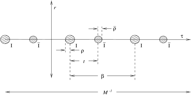
FIG. 3.: A sketch of periodic instanton-antiinstanton configurations. The $r$ axis represents the spatial distance from the origin, while the $\tau$ axis is imaginary time. The circles $I$ are instantons, of size $\rho$, while the circles $\bar{I}$ are antiinstantons, of size $\bar{\rho}$. The distance from an instanton to the nearest antiinstanton is $t$, while the period is $\beta$. To construct such a solution iteratively, $\rho$ and $\bar{\rho}$ must be small compared to $t$, $\beta$, or $\beta{-}t$, which in turn must be much shorter than the inverse mass scales of the theory, labeled here as $M^{-1}$.

To leading order, the fields of an instanton centered at the origin in singular gauge are [1]

$$A_{\mu}(x) = \frac{2\rho^{2}}{x^{2}(\rho^{2}+x^{2})}\,\bar{\eta}^{a}_{\mu\nu}x_{\nu}(\tau^{a}/2i)\>[1+{\mathcal{O}}(M_{W}x)],$$ (24)

$$\Phi(x) = \frac{\sqrt{2}M_{W}\,x}{\sqrt{x^{2}+\rho^{2}}}\>\xi\>[1+{\mathcal{O}}(M_{W}x)+{\mathcal{O}}(M_{H}x)],$$ (25)

where $\xi$ is an arbitrary complex unit doublet, and $\bar{\eta}^{a}_{\mu\nu}$ denotes ’t Hooft’s $\eta$ symbol [1]. The action of this field configuration, to leading order in the small parameter $M\rho$ (where $M$ denotes either $M_{W}$ or $M_{H}$) is

$$S_{I}=\frac{8\pi^{2}}{g^{2}}+\frac{4\pi^{2}}{g^{2}}M_{W}^{2}\rho^{2}+{\mathcal{O}}(M^{4}\rho^{4})\,.$$ (26)

The ${\mathcal{O}}(M_{W}^{2}\rho^{2})$ correction to the zero-order instanton action is due to the derivative term for the Higgs field, and is readily calculated as a surface integral [1]. The neglected ${\mathcal{O}}(M^{4}\rho^{4})$ contribution comes from the Higgs potential.

Consider placing such an instanton and antiinstanton along the time axis a distance $t$ apart. Since the fields approach their vacuum values for large distances $t\gg\rho$, one can construct an approximate solution to the equations of motion by linear superposition. Furthermore, if $\rho,\bar{\rho}\ll t\ll M^{-1}$, the leading interaction term between an instanton and an antiinstanton has the dipole-dipole form of the pure gauge theory [16]. It is

$$\Delta S_{I\bar{I}}=-\frac{1}{g^{2}}\left[\frac{96\pi^{2}\rho^{2}\bar{\rho}^{2}}{t^{4}}+{\mathcal{O}}(\rho^{6}/t^{6})+{\mathcal{O}}(M_{W}\rho^{4}/t^{3})\right]\,,$$ (27)

when the group orientations of the instanton and antiinstanton are aligned to give the maximally attractive interaction. This dipole interaction arises from the pure gauge field part of the action, and may be calculated as a simple surface integral. The interaction term for two instantons, or two antiinstantons, vanishes to this order.

For a periodic chain of alternating instantons and antiinstantons, such as the one illustrated in figure 3, there is a dipole interaction between each instanton and antiinstanton. Summing over all of these interactions yields, for the action per period of the periodic instanton-antiinstanton,

$$S_{I\bar{I}}(\rho,\bar{\rho},t;\beta) = \frac{4\pi^{2}}{g^{2}}\left[4+M_{W}^{2}(\rho^{2}{+}\bar{\rho}^{2})-\frac{\rho^{2}\bar{\rho}^{2}}{\beta^{4}}\sum_{n=-\infty}^{\infty}\frac{24}{(n+t/\beta)^{4}}\right]$$ (28)

$$= \frac{4\pi^{2}}{g^{2}}\left[4+M_{W}^{2}(\rho^{2}{+}\bar{\rho}^{2})-\frac{8\pi^{4}\rho^{2}\bar{\rho}^{2}}{\beta^{4}}\left(\frac{3{-}2\sin^{2}(\pi t/\beta)}{\sin^{4}(\pi t/\beta)}\right)\right]\,,$$ (29)

neglecting corrections of order $\rho^{6}/\beta^{6}$, $M^{4}\rho^{4}$, and $M_{W}\rho^{4}/\beta^{3}$. This expression is stationary with respect to variations of $t$ when $t=\beta/2$. Requiring the derivatives with respect to $\rho$ and $\bar{\rho}$ to vanish then fixes

$$\rho=\bar{\rho}={\sqrt{2}M_{W}\beta^{2}\over 4\pi^{2}}\,,$$ (30)

so that the classical action per period is

$$S(\beta)={1\over g^{2}}\left[16\pi^{2}+\frac{M_{W}^{4}\beta^{4}}{2\pi^{2}}+{\mathcal{O}}(M_{W}^{5}\beta^{5})\right].$$ (31)

This periodic solution has two negative modes. One negative mode, due to the attraction between the instanton and antiinstanton, is obvious because the action (29) is maximized with respect to $t$. The other negative mode is a symmetric perturbation $\delta\rho=\delta\bar{\rho}$ in instanton and antiinstanton sizes. This can be easily verified by noting that the mixed second derivative

$$\left.\frac{\partial^{2}S}{\partial\rho\,\partial\bar{\rho}}\right|_{\mathrm{e}xtremum}=-\frac{16\pi^{2}M_{W}^{2}}{g^{2}}$$ (32)

is the only second derivative of $S$ involving $\rho$ or $\bar{\rho}$ which doesn’t vanish at the extremum of $S$. The right hand side of the mixed second derivative (32) is thus a negative eigenvalue of the curvature of $S$, with an eigenvector satisfying $\delta\rho=\delta\bar{\rho}$ (and $\delta t=0$). This second negative mode is a signature of the delicate balancing required to construct a genuine periodic solution out of widely separated instantons, which themselves are not solutions.

The periodic instanton-antiinstanton solutions are time-reversal even, and thus have turning points, where all of the time-reversal odd field components (and velocities) vanish. The turning points are located halfway between the instanton and antiinstanton (at the origin in figure 3), as is clear by observing that the time-reversed fields of an instanton are those of an antiinstanton, and vice versa. The turning point energy of these solutions vanishes as the period goes to zero. Both negative modes of the periodic instanton-antiinstanton solutions are parity odd and time-reversal even.

V Thermal “Bounces” Near the Sphaleron

The $SU(2)$-Higgs action (9) is time-reversal invariant. Solutions to the equations of motion must either be time-reversal invariant, or come in time-reversed pairs. The periodic bounces we are interested in are time-reversal invariant solutions. This means that, at some time during the period, all time-reversal odd quantities must vanish. These times correspond to classical turning points, at which the kinetic terms in the Lagrangian vanish, leaving just the potential energy.

At turning-point energies just below the sphaleron energy, the bounces will be small fluctuations away from the sphaleron. Therefore, they may be studied using classical time-dependent perturbation theory. Given a time-independent action functional $S[\phi]$ of fields generically denoted as $\phi$, and a static solution $\phi_{0}$ (the sphaleron) which satisfies the equation of motion $\delta S[\phi_{0}]=0$, consider adding a small periodic fluctuation $\delta\phi$, of period $\beta$, to $\phi_{0}$. The classical equation of motion can be expanded in powers of the small fluctuation $\delta\phi$:

$$0=\delta S[\phi] = \delta S[\phi_{0}+\delta\phi]$$ (33)

$$= S^{(2)}\cdot\delta\phi+\frac{1}{2!}\,S^{(3)}\cdot(\delta\phi)^{2}+\frac{1}{3!}\,S^{(4)}\cdot(\delta\phi)^{3}\,,$$ (34)

where the inner product implies summation over internal indices as well as integration over space-time, and we have defined a shorthand notation for variational derivatives of the action

$$S^{(n)}\equiv\delta^{n}S[\phi_{0}].$$ (35)

The leading order piece of the equation of motion (34) is

$$0=S^{(2)}\cdot\delta\phi+{\mathcal{O}}\Bigl{(}(\delta\phi)^{2}\Bigr{)}.$$ (36)

This implies that the curvature $S^{(2)}$ has (at least) one eigenvalue of magnitude ${\mathcal{O}}(\delta\phi)$; that is, which becomes zero in the limit of vanishing fluctuation amplitude. This zero crossing of a curvature eigenvalue occurs at, and defines, the critical period $\beta_{0}$. The presence of a zero mode at the bifurcation point was pointed out in the context of the pendulum model; here we see its necessity from perturbation theory. We will label this particular eigenvalue $\lambda(\beta)$, explicitly indicating its dependence on the period of the fluctuation, so that

$$\lambda(\beta)=\lambda^{\prime}(\beta_{0})\,(\beta-\beta_{0})+{\mathcal{O}}\Bigl{(}(\beta{-}\beta_{0})^{2}\Bigr{)}\,.$$ (37)

Let $\eta(\beta)$ denote the corresponding eigenmode, so that

$$S^{(2)}\cdot\eta(\beta)=\lambda(\beta)\,\eta(\beta)\,.$$ (38)

To leading order, $\delta\phi$ consists of an undetermined (small) amount of the zero mode $\eta(\beta_{0})$.

To solve for $\delta\phi$ iteratively, beyond this linearized order, we rewrite the equation of motion (34) using the projection operator onto the eigenmode $\eta$, denoted $P_{\eta}$, to separate the small eigenvalue $\lambda$ when writing the inverse curvature ${S^{(2)}}^{-1}=P_{\eta}/\lambda+{S^{(2)}}^{-1}(1{-}P_{\eta})$. This gives

$$\delta\phi = -{S^{(2)}}^{-1}\cdot\left(\frac{1}{2!}\,S^{(3)}\cdot(\delta\phi)^{2}+\frac{1}{3!}\,S^{(4)}\cdot(\delta\phi)^{3}\right)$$ (39)

$$= \epsilon\,\eta-{S^{(2)}}^{-1}(1-P_{\eta})\cdot\left(\frac{1}{2!}\,S^{(3)}\cdot(\delta\phi)^{2}+\frac{1}{3!}\,S^{(4)}\cdot(\delta\phi)^{3}\right),$$ (40)

where the second line of this expansion (40) follows from the definition

$$\epsilon\equiv-\frac{1}{\lambda}\,\eta\cdot\left(\frac{1}{2!}\,S^{(3)}\cdot(\delta\phi)^{2}+\frac{1}{3!}\,S^{(4)}\cdot(\delta\phi)^{3}\right)\,.$$ (41)

(For convenience, we have assumed that the eigenmode $\eta(\beta)$ is normalized to one.) Defined in this way, $\epsilon$ is of magnitude ${\mathcal{O}}(\delta\phi)$, and will be used as a small parameter in the expansion (40).

The last line of the expansion (40) defines a recursive recipe for computing $\delta\phi$ as a power series in the small parameter $\epsilon$. Each place $\delta\phi$ occurs in the last line, one may substitute an entire copy of the last line, stopping at whatever power of $\epsilon$ is appropriate. This expansion is most conveniently written as a series of tree graphs, in which $n$-point vertices (for $n=3$ and $4$) correspond to $-S^{(n)}$, leaves (—$\!\bullet$) emerging from any vertex represent factors of $\epsilon\eta$, and internal lines correspond to the propagator ${S^{(2)}}^{-1}(1{-}P_{\eta})$. Each graph is to be divided by the usual symmetry factor, given by the number of permutations of leaves or vertices which leave the graph unchanged.

Carrying out the iterative expansion (40) explicitly to ${\mathcal{O}}(\epsilon^{3})$ gives us

$$\delta\phi=\;\raisebox{-15.89948pt}{\psfig{}}\;+\;\raisebox{-15.89948pt}{\psfig{}}\;+\;\raisebox{-15.89948pt}{\psfig{}}\;+\;\raisebox{-15.89948pt}{\psfig{}}\;+\;{\mathcal{O}}(\epsilon^{4})\,.$$ (42)

The graphical expansion (42) shows the beginning of the perturbative series for the field fluctuation $\delta\phi$ in the small parameter $\epsilon$ which may be used to characterize its size. But the parameter $\epsilon$ is not independent of the oscillation period $\beta$. The defining equation (41) relates the value of $\epsilon$ to the period $\beta$, and may be used to generate a perturbative expansion of the period $\beta$ in powers of $\epsilon$. To see how this goes, expand equation 41 using the same graphical expansion for $\delta\phi$,

$$\epsilon^{2}\lambda=3\left(\;\raisebox{-15.89948pt}{\psfig{}}\;\right)\>+\>4\left(\;\raisebox{-15.89948pt}{\psfig{}}\;+\;\raisebox{-15.89948pt}{\psfig{}}\;\right)\>+\>{\mathcal{O}}(\epsilon^{5})\,.$$ (43)

In fact, all diagrams in the expansion (43) with odd powers of $\epsilon$ (and hence $\eta$) vanish. This is because these diagrams imply integration over all time variables, and $\eta$ has a definite frequency $\beta^{-1}$, as will be seen explicitly in the following section. To fully expand the left-hand side of the $\lambda$ equation (43), use the expansion (37) for the eigenvalue $\lambda(\beta)$ and then expand $\beta{-}\beta_{0}$ in powers of $\epsilon$. Since, as noted above, only even powers of $\epsilon$ occur on the right-hand side of Eq. (43), the same must be true in the expansion of the period $\beta$,

$$\beta-\beta_{0}=\beta^{(1)}\epsilon^{2}+\frac{1}{2!}\,\beta^{(2)}\epsilon^{4}+\frac{1}{3!}\,\beta^{(3)}\epsilon^{6}+\cdots$$ (44)

Substitute the period expansion (44) into the eigenvalue expansion (37), substitute the result into the $\lambda$ equation (43), and match corresponding powers of $\epsilon$. The leading order result is

$$\epsilon^{4}\,\lambda^{\prime}(\beta_{0})\,\beta^{(1)}=4\left(\raisebox{-15.89948pt}{\psfig{}}\;+\;\raisebox{-15.89948pt}{\psfig{}}\right)\,,$$ (45)

or more explicitly,

$$\beta^{(1)}=\frac{1}{\lambda^{\prime}(\beta_{0})}\left[\frac{1}{2}\left(S^{(3)}\cdot\eta^{2}\right)\cdot{S^{(2)}}^{-1}(1{-}P_{\eta})\cdot\left(S^{(3)}\cdot\eta^{2}\right)-\frac{1}{3!}\,S^{(4)}\cdot\eta^{4}\right]\,,$$ (46)

where all quantities may now be evaluated at the critical period $\beta_{0}$.

VI Computation

We will evaluate equation (46) for perturbations about the sphaleron in $SU(2)$-Higgs theory, in order to find the leading-order dependence of the period of sphaleron oscillations on the amplitude $\epsilon$ of the fluctuating fields. We will also evaluate the leading order dependence of the turning point energy on the amplitude $\epsilon$ in order to re-express dependence on $\epsilon$ as dependence on the turning point energy.

To carry this out, one must discretize the radial dependence in the action (22), solve for the static sphaleron, determine the critical period $\beta_{0}$ and the leading order fluctuation $\eta(\beta_{0})$ by finding the zero-crossing eigenmode of the curvature $S^{(2)}$ evaluated at the sphaleron, and then assemble the various pieces needed to compute (46).

Since we are looking for periodic solutions, the time dependence of each of the fields appearing in the field equation (42) may be expanded in a Fourier series. Because $S^{(2)}$ is a time-independent linear operator, only the vertices $S^{(3)}$ and $S^{(4)}$ generate couplings between different harmonics. For the calculation of $\beta^{(1)}$, only field components at frequencies $0$, $\beta_{0}^{-1}$, and $2\beta_{0}^{-1}$ are needed.

Fixing a gauge is required, so as to remove zero modes of the curvature due to the residual $U(1)$ gauge invariance. There are two obviously reasonable choices: radial gauge ($a_{1}=0$), or temporal gauge ($a_{0}=0$). We chose to work in radial gauge, in order to avoid having to introduce link variables in the one-dimensional radial lattice.

Because the action, and the sphaleron in our choice of gauge, are parity (or $U(1)$ charge conjugation) even, it is useful to separate the fluctuating fields into parity even and odd components. The first order fluctuation $\eta$ is entirely odd. Each diagram in the field equation (42) then produces a contribution which is even if the number of leaves is even, and odd if the number of leaves is odd. The curvature $S^{(2)}$ is block-diagonal, and only the parity even block is needed for (46). Since the zero mode $\eta(\beta_{0})$ is parity odd, the projection operator $(1{-}P_{\eta})$ has no effect on the parity even block of the propagator.

Table II shows the discrete symmetries and leading order perturbative expansions of the real fields appearing with this choice of gauge. Note that all time derivatives appearing in the action, or its variations, may be trivially computed analytically.

The spatial derivatives in the action (22) were discretized using a uniform sampling of the transformed radial variable [13]

$$s=\ln\left[\frac{1+M_{H}r}{1+M_{W}r}\right]\Big{/}\ln(M_{H}/M_{W}),$$ (47)

which maps the semi-infinite line $0\leq r<\infty$ onto the unit interval $0\leq s<1$. Once the action is discretized, the sphaleron field, and the variations of the action at the sphaleron, can be computed as functions of the period.

Field	P	T	Leading Order Terms
$\alpha(r,t)$	$+$	$+$	$\alpha_{\mathrm{s}ph}(r)+\epsilon^{2}\left[\alpha^{(0)}(r)+\alpha^{(2)}(r)\cos(2\omega t)\right]$
$\mu(r,t)$	$+$	$+$	$\mu_{\mathrm{s}ph}(r)+\epsilon^{2}\left[\mu^{(0)}(r)+\mu^{(2)}(r)\cos(2\omega t)\right]$
$\beta(r,t)$	$-$	$+$	$\epsilon\,\beta^{(1)}(r)\cos(\omega t)$
$\nu(r,t)$	$-$	$+$	$\epsilon\,\nu^{(1)}(r)\cos(\omega t)$
$a_{0}(r,t)$	$-$	$-$	$\epsilon\,a_{0}^{(1)}(r)\sin(\omega t)$

TABLE II.: Symmetry properties, and leading order terms, of the field components for small oscillations about the sphaleron. $P$ is parity (or equivalently $U(1)$ charge conjugation), $T$ is time reversal, and a $+$ or $-$ indicates whether the field is even or odd, respectively, under the symmetry. The static sphaleron fields are labeled $\alpha_{\mathrm{s}ph}$ and $\mu_{\mathrm{s}ph}$. The fundamental angular frequency $\omega$ is $2\pi/\beta_{0}$, where $\beta_{0}$ is the critical period. The zero eigenmode $\eta(\beta_{0})$ is composed of the leading order terms for the parity odd fields $\beta$, $\nu$, and $a_{0}$. Note that only even powers of $\epsilon$ occur in the expansions for parity even fields, and only odd powers of $\epsilon$ appear in parity odd fields.

In particular, the curvature of the action is a matrix which, if inverted at the critical period, with the zero mode projected out, would give the propagator. In practice, it is computationally inefficient to actually calculate the matrix inverse. Since the action is local, discretizing the radial derivatives as nearest-neighbor differences gives the curvature matrix a band diagonal structure. Band diagonal algorithms for finding eigenvalues and solving linear equations have a computational cost which scales only linearly with the matrix dimension. An algorithm for band diagonal matrices [17] was used to find the eigenvalues of the curvature matrix, including $\lambda(\beta)$. Another band diagonal algorithm [18] was used to solve the linear equations $S^{(2)}\cdot z=\zeta$, with $\zeta=S^{(3)}\cdot\eta^{2}$. The same linear band algorithm was employed to find the sphaleron fields $\mu_{\mathrm{s}ph}$ and $\alpha_{\mathrm{s}ph}$ by Newton’s method iterations, and to generate the eigenvector $\eta(\beta)$ by inverse iteration [18].

As noted above, the variation $\beta^{(1)}$ of period with amplitude (46) may be converted into the variation in the period of the bounce with respect to the turning point energy, at the sphaleron. Explicitly,

$$\frac{\partial\beta}{\partial E}=\beta^{(1)}\left({\partial E\over\partial\epsilon^{2}}\right)^{-1}.$$ (48)

Since the kinetic terms of the Lagrangian vanish at the turning points, the variation of the turning point energy with amplitude $\partial E/\partial\epsilon^{2}$ is computed as the inner product

$$\frac{\partial E}{\partial\epsilon^{2}}(\beta_{0})=\frac{1}{\beta_{0}}\,\eta_{\mathrm{t}p}(\beta_{0})\,\cdot\,S^{(2)}\,\cdot\,\eta_{\mathrm{t}p}(\beta_{0})\,,$$ (49)

where $\eta_{\mathrm{t}p}(\beta_{0})$ are static fields equal to the turning point values of $\eta(\beta_{0})$. Similarly, the derivative with respect to period of the eigenvalue $\lambda^{\prime}(\beta_{0})$ appearing in the $\beta^{(1)}$ equation (46) is computed as the inner product

$$\lambda^{\prime}(\beta_{0})=\eta(\beta_{0})\,\cdot\,\frac{\partial S^{(2)}}{\partial\beta}\,\cdot\,\eta(\beta_{0})\;.$$ (50)

VII Numerical Results

Figure 4 shows the dependence of the critical period $\beta_{0}$ of oscillations on the Higgs mass $M_{H}$. The critical period was found by adjusting an arbitrarily large period $\beta$ down until the eigenvalue of the oscillating negative mode of the curvature matrix $S^{(2)}$ crossed zero.

Figure 5 shows the action of the sphaleron for one critical period $\beta_{0}$ as a function of the Higgs mass $M_{H}$. The sphaleron action was calculated by simply multiplying the sphaleron energy by the critical period $\beta_{0}$. This plot is important for understanding the connection between the sphaleron oscillations and the periodic instanton-antiinstanton solutions which occur at very short periods. The minimum action of these small instanton-antiinstanton solutions over one period, which is $4\pi/\alpha_{W}$, is shown as the dashed horizontal line on the graph. The sphaleron action crosses this minimal instanton-antiinstanton action when $M_{H}\approx 6.665\,M_{W}$.

FIG. 4.: The critical period of sphaleron oscillations $\beta_{0}$ vs. the Higgs mass $M_{H}$.

FIG. 5.: The action of the sphaleron over a single critical period vs. the Higgs mass $M_{H}$. The dashed horizontal line shows the minimum action of an instanton-antiinstanton solution.

Figure 6 shows the derivative of the period with respect to the turning point energy, $\partial\beta/\partial E$, as a function of the Higgs mass. At low Higgs mass, the derivative is positive, meaning that the oscillations move towards shorter periods as the turning point energy is decreased. At a Higgs mass of $3.091\,M_{W}$, the derivative crosses zero and thereafter becomes negative, meaning that for Higgs masses larger than this value oscillations move toward periods longer than $\beta_{0}$ as the turning point energy is initially decreased from the sphaleron energy.

FIG. 6.: The derivative of the period of small sphaleron oscillations with respect to the turning point energy vs. the Higgs mass $M_{H}$.

VIII Stability

Unstable modes of the bounce solution are closely related to those of the sphaleron. The sphaleron has a single static negative mode [13]. For periods shorter than the critical period $\beta_{0}$, this is its only negative mode. For periods $\beta$ longer than $\beta_{0}$, the sphaleron has two additional negative modes with frequency $\omega=2\pi/\beta$, given by the eigenmode $\eta(\beta)$ and its time derivative $\partial_{t}\eta(\beta)$.

Figure 7 illustrates the landscape of the action near the sphaleron and nearby bounce solutions, in the subspace spanned by $\delta\phi$ and its time derivative $\partial_{t}\delta\phi$. The action is represented by the height of the surface in each graph. The periodic time translation symmetry is represented as the rotational symmetry around the vertical axis. Classical solutions appear as peaks, cups, or saddle points. The sphaleron sits on the symmetry axis, because it is time translation invariant. The direction corresponding to the static negative mode of the sphaleron is not shown.

As shown in figure 7, when $\beta<\beta_{0}$, bounce solutions appear as a circular ridge around the sphaleron and have two negative modes (one of which is a small perturbation of the static negative mode of the sphaleron, and is suppressed in figure 7), plus a time-translation zero mode. When $\beta>\beta_{0}$, bounce solutions appear as a circular valley around the sphaleron and have only one near-static negative mode plus the time-translation zero mode. Both the near-static negative mode of the bounce, and the additional negative mode for $\beta<\beta_{0}$ (which is a small perturbation of $\eta(\beta_{0})$) are parity odd and time-reversal even.

	$\beta<\beta_{0}$	$\beta>\beta_{0}$
$\displaystyle\frac{\partial\beta}{\partial E}(\beta_{0})>0$
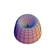
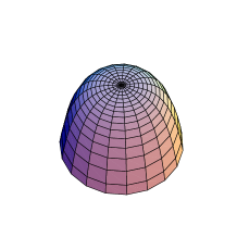
	$\kappa_{S}=1\qquad\kappa_{B}=2$	$\kappa_{S}=3$
$\displaystyle\frac{\partial\beta}{\partial E}(\beta_{0})<0$
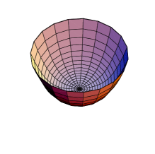
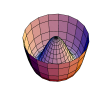
	$\kappa_{S}=1$	$\kappa_{S}=3\qquad\kappa_{B}=1$

FIG. 7.: Topography of the action near the sphaleron and nearby bounce solutions. The height of the surface in each graph represents the action. The extremum of the action on the axis of rotational symmetry is the sphaleron. The other extrema are the periodic bounce solutions, and have a time translation zero mode represented by rotations about the symmetry axis. $\kappa_{S}$ denotes the number of unstable modes of the sphaleron, while $\kappa_{B}$ is the number of unstable modes of the bounce. The action has one additional unstable direction, not shown in the figure, corresponding to the static unstable mode of the sphaleron.

IX Discussion

The results shown in figures 5 and 6, when taken together with the analytic results on short-period periodic instantons, allow one to suggest a picture of the branches of periodic, spherically symmetric, Euclidean classical solutions of this theory, which will be illustrated on the following plots of action versus period. On such plots, periodic classical solutions trace out curves, the slope of which at any point is equal to the conserved energy of the solution. The sphaleron, as a static solution, appears as a straight line through the origin, with a slope given by the energy of the sphaleron. Bounces with turning points have a slope equal to their turning-point energy, and thus must always have a positive slope. Solutions may merge (at bifurcation points where curvature eigenvalues pass through zero) when the curves representing the solutions meet at tangent points on the plot. The curves must be tangent for the solutions to have the same conserved energy.

FIG. 8.: Euclidean classical solutions of the $SU(2)$-Higgs model, sketched on plots of action versus period, for three different values of the Higgs mass. On these plots, slope is equal to turning-point energy. The plots are drawn for purposes of illustration, and are not to scale. The line through the origin is the sphaleron. The curve of bounces $C$ merges with the sphaleron at the point $Q$, which is at the critical period $\beta_{0}$. For periods very short compared with the inverse mass scales ($M_{H}^{-1}$, $M_{W}^{-1}$) of the theory, there exist periodic instanton-antiinstanton solutions $I$ with near-zero turning point energy.

Figure 8 summarizes the perturbative results for the bounces and periodic instanton-antiinstantons found in this paper, for three different values of the Higgs mass. These schematic plots of action versus period are not drawn to scale. The curve of bounces $C$ merges with the sphaleron line at point $Q$, which is at the critical period $\beta_{0}$. For periods very short compared with the inverse mass scales ($M_{H}^{-1}$, $M_{W}^{-1}$) of the theory, there exist periodic instanton-antiinstanton solutions $I$ with near-zero turning point energy. For brevity, we will henceforth call these, in an abuse of language, periodic instantons.

For light Higgs (less than $3.091\,M_{W}$), figure 8(a) shows that the bounces $C$ decrease in period as their turning point energy is decreased from the sphaleron energy. This is clear from figure 6 for small Higgs mass. On the same plot, the action at point $Q$ is larger than the minimum action of the periodic instantons $I$. This one can read from figure 5 in the limit of small Higgs mass.

As noted in figure 6, above a Higgs mass of $3.091\,M_{W}$, the bounces $C$ increase in period as their turning point energy is lowered from the sphaleron energy. This situation is illustrated in figure 8(b).

From figure 5 we note that as the Higgs mass is increased, the action at point $Q$ decreases, because the period $\beta_{0}$ shrinks faster than the sphaleron energy grows. When the Higgs mass reaches $6.665\,M_{W}$, the action at point $Q$ crosses below the minimum action of the periodic instantons $I$, that is, $4\pi/\alpha_{W}$. This situation is shown in figure 8(c).

Given this information available from perturbative calculations about the branches of periodic instantons and bounces, one can construct a likely scenario for the behavior of the various solutions in between the known limits.

For a sufficiently light Higgs mass, where the situation shown in figure 8(a) holds, it is obviously simplest to assume that the branch of periodic instanton solutions $I$ and the branch of bounces $C$ are one and the same. We illustrate this hypothesis in figure 9(a), where the dotted line indicates the single hypothetical branch of solutions. Both of the solutions $I$ and $C$ have two parity odd, time-reversal even negative modes, which is an important consistency check on this picture. This picture of a single branch of periodic solutions interpolating between the short-period instanton-antiinstanton solution and the sphaleron at its critical period is precisely the situation which occurs in the two-dimensional non-linear $O(3)$ sigma model with a symmetry breaking mass term [5].

When the Higgs mass exceeds the value $3.091\,M_{W}$, as discussed above, the bounce period increases as the turning point energy is decreased from the sphaleron energy. The simplest explanation for this, drawn from analogy with the toy model, is shown in figure 9(b). A new bifurcation point $P$ appears, where the branch of bounces $C$ and the branch of periodic instantons $I$ merge, at a period longer than $\beta_{0}$.

When the Higgs mass reaches the value $6.665\,M_{W}$, as noted above, the action at point $Q$ is equal to the minimum action of the periodic instantons $I$. This situation is illustrated in figure 9(c). This implies that, to exponential accuracy, the bounces set the rate of barrier penetration for the range of periods for which their action is below the periodic instanton action.

As discussed earlier, bounces emerging from the sphaleron with $\beta>\beta_{0}$ have only a single negative mode (which is parity odd and time-reversal even). Hence the branch $QP$ for $M_{H}>3.091\,M_{W}$ will have only a single negative mode. Point $P$ is thus a typical example of a bifurcation where real solutions with stabilities differing by $\pm 1$ merge.

FIG. 9.: The simplest scenario for Euclidean classical solutions of the $SU(2)$-Higgs model consistent with the known perturbative results of figure 8. The number next to each branch of solutions gives the number of unstable directions. (a) For Higgs mass lighter than $3.091\,M_{W}$, the periodic instantons and bounces are joined by a single branch of solutions, indicated here by a dotted line. (b) For a Higgs mass above $3.091\,M_{W}$, the periodic instantons and bounces meet at a new bifurcation point $P$. (c) When the Higgs mass exceeds $6.665\,M_{W}$, the action at point $Q$ is less than the action of the periodic instantons $I$.

To exponential accuracy, the rate of barrier penetration at a given temperature $\beta^{-1}$ in each of the plots in figure 9 is set by the lowest action configuration with period $\beta$, except that there is an additional lower limit set by the zero size limit of periodic instanton configurations, which, for any period, have a limiting action of $4\pi/\alpha_{W}$. Thus, in cases (a) and (b), there is an abrupt crossover from a sphaleron-dominated rate at higher temperatures to a singular instanton-dominated rate at lower temperatures. In case (c), there is a smooth transition from the sphaleron to the branch $QP$, followed by an abrupt transition to singular instantons.

Note Added

The above scenario for periodic Euclidean solutions of $SU(2)$-Higgs theory has recently been confirmed by direct numerical studies of time-dependent (spherically symmetric) periodic solutions [19, 20].

REFERENCES

- [1] G. ’t Hooft, Phys. Rev. D 14, 3432 (1976).
- [2] F. R. Klinkhamer and N. S. Manton, Phys. Rev. D 30, 2212 (1984).
- [3] V. A. Kuzmin, V. A. Rubakov, and M. E. Shaposhnikov, Phys. Lett. 155B, 36 (1985).
- [4] P. Arnold and L. McLerran, Phys. Rev. D 37, 1020 (1988).
- [5] S. Habib, E. Mottola, and P. Tinyakov, Phys. Rev. D 54, 7774 (1996).
- [6] A. Kuznetsov and P. Tinyakov, Phys. Lett. B406, 76 (1997).
- [7] S. Coleman, Phys. Rev. D 15, 2929 (1977).
- [8] C. G. Callan and S. Coleman, Phys. Rev. D 16, 1762 (1977).
- [9] I. Affleck, Phys. Rev. Lett. 46, 388 (1981).
- [10] S. Y. Khlebnikov, V. A. Rubakov, and P. G. Tinyakov, Nucl. Phys. B 367, 334 (1991).
- [11] L. D. Landau and E. M. Lifshitz, Mechanics, 3rd ed. (Pergamon Press, New York, 1976).
- [12] B. Ratra and L. G. Yaffe, Phys. Lett. B205, 57 (1988).
- [13] L. G. Yaffe, Phys. Rev. D 40, 3463 (1989).
- [14] J. Kunz and Y. Brihaye, Phys. Lett. B216, 353 (1989).
- [15] S. Coleman, Aspects of Symmetry (Cambridge University Press, New York, 1988).
- [16] C. G. Callan, R. F. Dashen, and D. J. Gross, Phys. Rev. D 17, 2717 (1978).
- [17] H. R. Schwarz, Numer. Math. 12, 231 (1968).
- [18] R. S. Martin and J. H. Wilkinson, Numer. Math. 9, 279 (1967).
- [19] K. L. Frost and L. G. Yaffe, in preparation.
- [20] S. Habib, E. Mottola, C. Rebbi, R. Singleton, and P. Tinyakov, private communication.