DTP/98/50

July 1998

Saturation Effects in Deep Inelastic Scattering
at low $Q^{2}$ and its Implications on Diffraction
K.  Golec-Biernat and M. Wüsthoff

Department of Physics, University of Durham, Durham DH1 3LE, UK

()

We present a model based on the concept of saturation for small $Q^{2}$ and small $x$. With only three parameters we achieve a good description of all Deep Inelastic Scattering data below $x=0.01$. This includes a consistent treatment of charm and a successful extrapolation into the photoproduction regime. The same model leads to a roughly constant ratio of diffractive and inclusive cross section.

1 Introduction

The basic concept of saturation in Deep Inelastic Scattering (DIS) is related to the transition from high to low $Q^{2}$ as one observes in the total $\gamma^{*}p$-cross section. This type of saturation occurs when the photon wavelength $1/Q$ reaches the size of the proton. We will include another aspect of saturation in our paper which is inherent to DIS at small $x$ (small-$x$ saturation). In this regime the partons in the proton form a dense system with mutual interaction and recombination which also leads to the saturation of the total cross section [1]. Both aspects of saturation are closely linked to confinement and unitarity. While the latter might be approached perturbatively [2], the first is genuinely nonperturbative. The approach we choose here can be called QCD-inspired phenomenology and follows the line of refs.[3, 4, 5]. It is in spirit most similar to the ideas of the analysis [6].

The basis for our approach is the fact that the photon splits up into a quark-antiquark pair (dipole), far upstream the proton target, which then scatters on the proton. In the pure perturbative regime the reaction is mediated by single-gluon exchange which changes into multi-gluon exchange when the saturation region is approached. The latter process can be interpreted as the interaction with a ’semiclassical field’ [7]. Most important for us is the fact that the mechanism leading to the dissociation of the photon and the subsequent scattering can be factorized and written in terms of a photon wave function convoluted with a quark-antiquark cross section $\hat{\sigma}$ [8]. In our analysis this cross section has the simple form $\hat{\sigma}=\sigma_{0}\{1-exp[-r^{2}/(4R_{0}^{2}(x))]\}$ where $r$ denotes the separation between the quark and antiquark and $R_{0}^{2}$ is the $x$-dependent saturation scale: $R_{0}^{2}(x)=(x/x_{0})^{\lambda}$. The functional form of $\hat{\sigma}$ can be different, important is, however, that for small $r$ it is proportional to $r^{2}$ (colour transparency) while for large $r$ the cross section approaches a constant value. The latter behaviour ensures saturation. The crucial element in our analysis is the assumption that the saturation scale $R_{0}$ depends on $x$ in such a way that with decreasing $x$-Bjorken one has to go to smaller distances (higher $Q^{2}$) in order to resolve the dense parton structure of the proton. The boundary in the $(x,Q^{2})$-plane along which saturation sets in is described by the “critical line”, $Q^{2}=1/R_{0}^{2}(x)$.

The recent low-$Q^{2}$ data from HERA [9, 10] have triggered significant theoretical activity. In one class of models [11, 12] the description of the data is achieved by combining the nonperturbative vector meson contribution (VDM-model) with contributions based on perturbative QCD. Both models do not use the concept of small-$x$ saturation.

Another class of models [13, 14, 15] is based on Regge theory. The total cross section $\sigma^{\gamma^{*}p}$ is the sum of contributions from different Reggeons. In particular in ref.[13] the leading behaviour is given by the sum of two Pomeron contributions with “hard” and “soft” intercepts. Again the concept of the small-$x$ saturation is not implemented in these analyses. The claim in ref.[13] is that saturation at present energies is not needed. However, in the true high energy asymptotics something has to happen. The hard Pomeron as proposed in ref.[13] would eventually overtake and strongly violate unitarity. Other approaches like those in refs.[16, 17] have imposed a logarithmic behaviour in $x$ from the very beginning and thus do not violate unitarity.

The strategy we adopt in our analysis is the following. We determine the three free parameters of our model mentioned earlier, $\sigma_{0},\lambda$ and $x_{0}$, by fits to all existing DIS data for $x\leq 0.01$. We then study the obtained parameterization in the photoproduction region, where a non-zero quark mass is required to achieve a finite cross section. The quark mass is chosen such that the photoproduction cross section is in rough agreement with the data without having them included in our fit. We found that the effective slope $\lambda_{eff}$ of the cross section ($\sigma\sim(W^{2})^{\lambda_{eff}}$) interpolates between the “soft” Pomeron value $\approx 0.08$ and the “hard” value $\approx 0.29$. We would like to point out that the “soft” value is simply a result of the extrapolation of our fits to the photoproduction region. After a first fit with only light quark flavours we perform a second fit which includes charm. We found again a good description of all inclusive DIS data and in addition the correct relative charm contribution. The model we use can be straightforwardly applied to DIS diffractive processes leading to the interesting result that the ratio of the diffractive and inclusive cross section is roughly constant as a function of $x$ and $Q^{2}$.

The content of the paper is the following. In section 2 we introduce the theoretical details of the model and discuss its qualitative features. We then derive a simplified parameterization which illustrates the concept of the critical line. This parameterization can also serve for a quick fit to the data. In Section 3 we describe our two fits and discuss their physical implications. Section 4 is devoted to the study of diffraction based on our model and section 5 contains conclusions.

2 Models for Saturation

For small values of the Bjorken variable $x$ the photon wave function formalism has been established as useful tool for calculating deep inelastic and related diffractive cross sections for $\gamma^{*}p$ scattering [3, 4, 8]. It allows to separate between the wave function of the photon which describes the dissociation of the photon into a quark-antiquark pair and the interaction of the quark-antiquark pair with the target. The photon wave function constitutes the calculable part of the process whereas the remainder is substantially influenced by nonperturbative contributions and needs to be modelled. The corresponding diagram is shown in Fig. 1. We work in a frame where the photon with momentum $q$ and the proton with momentum $p$ are collinear. Accordingly, the distribution of the quark-antiquark pair is given in terms of $z$ and $(1-z)$, the momentum fraction with respect to $q$, and the relative transverse separation ${\bf r}$. For transverse $({T})$ and longitudinally $({L})$ polarized photons the $\gamma^{*}p$-cross section takes the form [4, 8]

Figure 1: Diagrammatical representation of the basic process as discussed in the text.

$$\sigma_{T,L}(x,Q^{2})\>=\>\int\!d\,^{2}{\bf r}\!\int_{0}^{1}\!dz\>|\Psi_{T,L}\,(z,{\bf r})|^{2}\>\hat{\sigma}\,(x,r^{2})\;,\\$$ (1)

where $W^{2}=(p+q)^{2}$, $Q^{2}=-q^{2}$ and $x=Q^{2}/(W^{2}+Q^{2})$. The squared photon wave function $\Psi_{T,L}$ is given by

$$|\Psi_{T}\,(z,{\bf r})|^{2}\>=\>\frac{6\,\alpha_{em}}{4\,\pi^{2}}\>\sum_{f}\,e_{f}^{2}\>\Big{\{}\,[\,z^{2}+(1-z)^{2}\,]\>\epsilon^{2}\,K_{1}^{2}\,(\epsilon\,r)\,+\,m_{f}^{2}\>K_{0}^{2}\,(\epsilon\,r)\,\Big{\}}$$ (2)

and

$$|\Psi_{L}\,(z,{\bf r})|^{2}\>=\>\frac{6\,\alpha_{em}}{4\,\pi^{2}}\>\sum_{f}\,e_{f}^{2}\>\Big{\{}\,4\,Q^{2}\,z^{2}\,(1-z)^{2}\,K_{0}^{2}\,(\epsilon\,r)\,\Big{\}}\;,$$ (3)

for the transverse and longitudinal photons, respectively. In the above formulae

$$\epsilon^{2}\>=\>z\,(1-z)\,Q^{2}\,+\,m_{f}^{2}\;.$$ (4)

$K_{0}$ and $K_{1}$ are Mc Donald functions and the summation is performed over the quark flavours. The $\gamma^{*}p$ cross sections are related to the structure function $F_{2}$ in the following way

$$F_{2}\,(x,Q^{2})\,=\,F_{T}\,(x,Q^{2})\,+\,F_{L}\,(x,Q^{2})$$ (5)

and

$$F_{T,L}\,(x,Q^{2})\,=\,\frac{Q^{2}}{4\,\pi^{2}\,\alpha_{em}}\;\sigma_{T,L}(x,Q^{2})\;.$$ (6)

The interaction of the $q\overline{q}$ pair with the proton is described by the dipole cross section $\hat{\sigma}\,(x,r^{2})$ which is modelled in our analysis. The most crucial element is the adoption of the $x-$dependent radius

$$R_{0}\,(x)\,=\,\frac{1}{Q_{0}}\;\Bigg{(}\frac{x}{x_{0}}\Bigg{)}^{\lambda/2}\;,$$ (7)

which scales the quark-antiquark separation $r$ in the dipole cross section

$$\hat{\sigma}\,(x,r^{2})\;=\;\sigma_{0}\;g\,(\hat{r}^{2})\;,$$ (8)

with

$$\hat{r}\;=\;\frac{r}{2\,R_{0}(x)}\;.$$ (9)

$Q_{0}=1~{}GeV$ in (7) sets the dimension. The function $g$ in (8) is not completely constrained. Important, however, is the quadratic rise at small $\hat{r}$ and the flattening off at large $\hat{r}$. The latter behaviour provides saturation of the cross section (1), i.e. $\sigma^{\gamma^{*}p}=\sigma_{T}+\sigma_{L}\sim const$ for small $Q^{2}$. At small $\hat{r}$, on the other hand, we have a simple scaling behaviour (colour transparency), $\sigma^{\gamma^{*}p}\sim 1/Q^{2}$, combined with a power-like dependence of (8) on $x$ as typically observed in deep inelastic scattering. We choose the following simple Ansatz for the function $g$

$$g\,(\hat{r}^{2})\;=\;1\,-\,e^{-\hat{r}^{2}}\;.$$ (10)

This Ansatz reminds of eikonalization. It should be mentioned, however, that a complete eikonal treatment requires the incorporation of a target profile function. The form (10) would mean in this context that the gluonic density in the proton is evenly distributed over a certain area within a sharp boundary and zero beyond. A more sophisticated treatment including a realistic profile function can be found in ref.[5, 6]. The corresponding result in these references can be roughly approximated by

$$g\,(\hat{r}^{2})\;=\;\ln(1+\hat{r}^{2})$$ (11)

and shows a logarithmic growth at large distances.

For small $z$ one can as well think of a logarithmic modification as is motivated by the single gluon exchange (see ref.[4])

$$g\,(\hat{r}^{2})\;=\;\hat{r}^{2}\ln\left(1+\frac{1}{\hat{r}^{2}}\right)\;\;.$$ (12)

Both alternatives (11) and (12) can be easily implemented in our formalism which we present in the forthcoming sections. It turns out, however, that they are disfavoured in our analysis and we will not discuss them in detail. This does not mean that we contradict their physical implications. It might be that a different approach could be reconciled with the models (11) or (12).

In our analysis we fit the three parameters, $\sigma_{0}$, $x_{0}$ and $\lambda$, of the dipole cross section (8) and (10). Before going into the details of the fits it is illuminating to perform a qualitative analysis of the behaviour of the cross section (1) in our model.

2.1 Qualitative Analysis

In the following discussion we focus on the cross section $\sigma_{T}$ in (1) which dominates over $\sigma_{L}$. We also neglect for simplicity the quark mass. The important point in the qualitative analysis is the behaviour of $K_{1}(\epsilon\,r)$ in (2) for small values of $\epsilon\,r$:

$$K_{1}(\epsilon\,r)\,\sim\,\frac{1}{\epsilon\,r}\;.$$ (13)

For large values of $\epsilon\,r$ the function $K_{1}$ is exponentially suppressed. Thus in order to obtain the dominant contribution we perform the integration in (1) for $\epsilon\,r<1$.

The photon virtuality introduces the scale $1/Q$ for the transverse dimension of the $q\overline{q}$ pair. A pair is considered “small” when the condition $r<1/Q$ is fulfilled and “large” when $r>1/Q$. Let us analyse the contribution to (1) coming from small pairs for which the condition $\epsilon\,r=\sqrt{z(1-z)}\,r\,Q<1$ is satisfied for all values of $z$. In the case $1/Q\ll R_{0}$, shown in Fig. 2a, the size of the small $q\overline{q}$ pairs is much smaller than the saturation radius and $\hat{\sigma}(r)\;\sim\;\sigma_{0}\,\hat{r}^{2}/R_{0}^{2}$. The cross section (1) exhibits the following behaviour

$$\sigma_{T}\>\sim\>\frac{\sigma_{0}}{R_{0}^{2}}\,\int dz\int\limits_{0}^{1/Q^{2}}d\,r^{2}\,\epsilon^{2}\,\Bigg{(}\frac{1}{\epsilon^{2}\,r^{2}}\Bigg{)}\,\hat{r}^{2}\;\;\sim\;\frac{1}{Q\,^{2}}\;\frac{\sigma_{0}}{R^{2}_{0}}$$ (14)

where the integration over $z$ could be factored after the cancellation of the $\epsilon$ factors. Thus for constant $x$ the cross section (14) exhibits the familiar short distance scaling behaviour, i.e the corresponding structure function $F_{2}(x,Q^{2})$ is roughly constant in $Q^{2}$.

Figure 2: The profile of the dipole cross section for different $Q$. The small arrows below the figure show how the indicated parameters change when $Q$ decreases (for $W^{2}$ fixed).

Let us now analyse the situation shown schematically in Fig. 2b in which the size of the $q\overline{q}$ pair is bigger than the saturation radius $1/Q>R_{0}$. For the small pair contribution to $\sigma_{T}$ we now obtain

$$\sigma_{T}\>\sim\>\int\limits_{0}^{R_{0}^{2}}d\,r^{2}\,\Bigg{(}\frac{1}{r^{2}}\Bigg{)}\,\sigma_{0}\,\frac{\,r^{2}}{R^{2}_{0}}\;+\;\int\limits_{R_{0}^{2}}^{1/Q^{2}}d\,r^{2}\,\Bigg{(}\frac{1}{r^{2}}\Bigg{)}\,\sigma_{0}\;\sim\;\sigma_{0}\,+\,\sigma_{0}\;\log\,\bigg{(}\frac{1}{Q^{2}\,R_{0}^{2}}\,\bigg{)}\;.$$ (15)

With respect to the power behaviour in $Q^{2}$ the cross section can be viewed as being constant. The potential divergence due to the logarithm will be regulated by the quark mass in our full analysis. The actual value of the mass plays an important role in the description of the photoproduction region.

A similar analysis can be performed for “large” pairs for which $r>1/Q$. The integration condition $\epsilon\,r<1$ is now satisfied when $z<1/(r^{2}\,Q^{2})$ and the $z$ integration in (1) can no longer be factored out. It has to be done before integrating over $r$. The result in the end is the same as for small pairs. If the characteristic size of the $q\overline{q}$ dipole is less than $R_{0}$ the scaling behaviour is obtained. For $1/Q\lower 3.01385pt\hbox{$\;\stackrel{{\scriptstyle\textstyle>}}{{\sim}}\;$}R_{0}$ the cross section $\sigma_{T}$ is constant in $Q^{2}$. A more detailed analysis gives logarithmic modifications.

So far in our discussion we have assumed a constant saturation radius which allows a smooth transition of $\sigma_{T}$ between the scaling region of large $Q^{2}$ and the saturation region of low $Q^{2}$ (low-$Q^{2}$ saturation). The main feature of our model, however, is the fact that the saturation radius $R_{0}$ depends on $x$ ($R_{0}(x)\sim x\,^{\lambda/2}$ with $\lambda>0$). In this way we have introduced another kind of saturation which can be called the small-$x$ saturation. In terms of the parton picture it is closely related to the saturation of the gluon density [19]. An important consequence is that for fixed $W$ the radius $R_{0}$ becomes $Q$ dependent which makes the saturation more dynamical. As illustrated in Fig. 2 both $R_{0}$ and $1/Q$ move towards each other, at a certain scale $Q=1/R_{0}$ they meet and then pass each other. Hence, the saturation occurs at higher values of $Q^{2}$ than in a model with a fixed $R_{0}$. In addition the transition from high to low $Q^{2}$ is faster. The line given by the condition

$$R_{0}^{2}(x)=\frac{1}{Q^{2}}$$ (16)

will be called the critical line. In the parton picture it would describe the boundary of the critical density [19]. The precise saturation pattern is determined by the fits of the three parameters in (8) to the existing DIS inclusive data.

2.2 The Mellin Transformation

In this section we briefly describe the technique we use to perform the fits. In order to evaluate the cross section (1) we employ the Mellin transformation to factorize the wave function from the cross section. This reduces the number of numerical integrations to one and allows for an easier discussion of the scaling behaviour:

$$\sigma_{T,L}(x,Q^{2}) = \int\frac{d\nu}{2\pi}\int\!d\,^{2}{\bf r}\int_{0}^{1}\!dz\;|\Psi_{T,L}\,(z,{\bf r})|^{2}\>\int\frac{dr^{\prime 2}}{r^{\prime 2}}\left(\frac{r}{r^{\prime}}\right)^{1+2i\nu}\sigma\,(\tilde{x},r^{\prime 2})$$

$$= \sigma_{0}\;\;\int\frac{d\nu}{2\pi}\;\;\left[\left(\frac{x_{0}}{\tilde{x}}\right)^{\lambda}\frac{Q_{0}^{2}}{Q^{2}}\right]^{1/2+i\nu}\mbox{H${}_{T,L}$}\left(\nu,\frac{m_{f}^{2}}{Q^{2}}\right)\;\;\mbox{G}(\nu)$$

where

$$\mbox{H${}_{T}$}\left(\nu,\frac{m_{f}^{2}}{Q^{2}}\right)=\sum_{f}e_{f}^{2}\;\frac{6\alpha_{em}}{2\pi}\;\frac{\sqrt{\pi}}{4}\;\frac{\Gamma^{2}(3/2+i\nu)\Gamma(1/2+i\nu)}{\Gamma(2+i\nu)}\;\left(\frac{Q^{2}+4m_{f}^{2}}{Q^{2}}\right)^{1/2-i\nu}$$

$$\times \left\{\left[\frac{(1+3i\nu)Q^{2}+(3+2i\nu)m_{f}^{2}}{Q^{2}+4m_{f}^{2}}-i\nu\left(\frac{Q^{2}}{Q^{2}+4m_{f}^{2}}\right)^{2}\right]\right.\;\mbox{${}_{2}F_{1}$}\left(\frac{1}{2}+i\nu,\frac{1}{2};\frac{3}{2};\frac{Q^{2}}{Q^{2}+4m_{f}^{2}}\right)$$

$$+\left[(1-i\nu)\frac{Q^{2}}{Q^{2}+4m_{f}^{2}}-\frac{3+2i\nu}{4}\right]\left.\;\mbox{${}_{2}F_{1}$}\left(-\frac{1}{2}+i\nu,\frac{1}{2};\frac{3}{2};\frac{Q^{2}}{Q^{2}+4m_{f}^{2}}\right)\right\}\;$$

and

$$\mbox{H${}_{L}$}\left(\nu,\frac{m_{f}^{2}}{Q^{2}}\right) = \sum_{f}e_{f}^{2}\;\frac{6\alpha_{em}}{2\pi}\;\frac{\sqrt{\pi}}{4}\;\frac{\Gamma^{3}(3/2+i\nu)}{\Gamma(2+i\nu)}\;\left(\frac{Q^{2}+4m_{f}^{2}}{Q^{2}}\right)^{-3/2-i\nu}$$

$$\times\frac{16}{30}\;\;\mbox{${}_{2}F_{1}$}\left(\frac{3}{2}+i\nu,\frac{1}{2};\frac{7}{2};\frac{Q^{2}}{Q^{2}+4m_{f}^{2}}\right)\;.$$

In addition in (2.2)

$$\\ \mbox{G}(\nu)\;=\;\int_{0}^{\infty}\;d\hat{r}^{2}\;\left(\hat{r}^{2}\right)^{-3/2-i\nu}\;\,g(\hat{r}^{2})\;\;\;.$$

In order to have the right threshold behaviour and a smooth transition in the limit $Q^{2}\rightarrow 0$ we also modify the Bjorken variable

$$\tilde{x}\;=\;x\;\frac{Q^{2}+4m_{f}^{2}}{Q^{2}}\;\;.$$ (20)

The Mellin transformation for the functional form (10) of the function $g$ which defines the dipole cross section in our analysis yields:

$$\mbox{G}(\nu)\;=\;-\Gamma(-\frac{1}{2}-i\nu)\;.$$ (21)

For the sake of completeness we also present the corresponding expressions for the alternative models in (11) and (12),

$${\mbox{G}}(\nu) = \frac{1}{1/2+i\nu}\;\frac{\pi}{\cosh(\pi\nu)}\;$$ (22)

and

$${\mbox{G}}(\nu) = \frac{1}{1/2-i\nu}\;\frac{\pi}{\cosh(\pi\nu)}\;.$$ (23)

The main purpose of introducing a mass is to have a finite limit $Q^{2}\rightarrow 0$. However in the region $Q\lower 3.01385pt\hbox{$\;\stackrel{{\scriptstyle\textstyle>}}{{\sim}}\;$}1~{}GeV$, where we mainly fit the data, the mass has little effect and one might as well consider the case with zero mass. In this case the functions (2.2) and (2.2) reduce to

$$\mbox{H${}_{T}$}(\nu,0)\;=\;\sum_{f}e_{f}^{2}\;\frac{6\alpha_{em}}{2\pi}\;\frac{\pi}{16}\;\frac{9/4+\nu^{2}}{1+\nu^{2}}\;\left(\frac{\pi}{\cosh(\pi\nu)}\right)^{2}\;\frac{\sinh(\pi\nu)}{\pi\nu}\;\frac{\Gamma(3/2+i\nu)}{-\Gamma(-1/2-i\nu)}$$ (24)

and

$$\mbox{H${}_{L}$}(\nu,0)\;=\;\sum_{f}e_{f}^{2}\;\frac{6\alpha_{em}}{2\pi}\;\frac{\pi}{8}\;\frac{1/4+\nu^{2}}{1+\nu^{2}}\;\left(\frac{\pi}{\cosh(\pi\nu)}\right)^{2}\;\frac{\sinh(\pi\nu)}{\pi\nu}\;\frac{\Gamma(3/2+i\nu)}{-\Gamma(-1/2-i\nu)}\;\;.$$ (25)

The results (24) and (25) are much simpler than in the massive case and probably familiar to those readers who have calculated the Mellin transform of the quark-box diagram in momentum space. The only difference is the ratio of the $\Gamma$ functions at the end of each expression which is a residue of the Fourier transform.

We use formulae (2.2) through (21) in our fits and perform the integration over $\nu$ numerically. The main virtue of this representation is the quick convergence of the integrand in (2.2) which makes the numerical integration very fast. Another virtue is the rather simple analytical structure which allows to extract the leading scaling behaviour of $\sigma_{T}$ for large as well as low $Q^{2}$, as will be demonstrated in the next section.

2.3 Simplified Parametrization and Critical Line

In this section we analyse the analytical structure of the cross section (2.2) in the complex $\nu$-plane. We use the formulae (24) and (25) for the massless case. The position and characteristics of the singularities in the complex $\nu$-plane determine the behaviour of the analysed cross section. In general the $\nu$-integration runs along the real axis, and depending on the argument $\left(\frac{x_{0}}{x}\right)^{\lambda}\frac{Q_{0}^{2}}{Q^{2}}$ in eq. (2.2) one can close the contour in the upper or lower part of the complex plane. For example, in the case of large $Q^{2}$ and not too small $x$ (“hard” regime) the mentioned argument is less than 1 and the contour has to be closed in the lower plane. The first singularity encountered is a pole at $\nu=-i/2$. Depending on the model for the dipole cross section given by (21), (22) or (23), it can be a double or triple pole. The model (21) used in our analysis leads to a double pole which generates a logarithmic behaviour of the cross section (2.2)

$$\left(\frac{x_{0}}{x}\right)^{\lambda}\frac{Q_{0}^{2}}{Q^{2}}\;\;\ln\left[\left(\frac{x}{x_{0}}\right)^{\lambda}\frac{Q^{2}}{Q_{0}^{2}}\right]\;\;.$$ (26)

One should note that the logarithm is due to the photon wave function (the quark-box diagram) and is related to the splitting of a gluon into a quark-antiquark pair. The factor in front of the logarithm arises because $1/2+i\nu=1$ in eq. (2.2) and simply reflects the basic scaling behaviour of $F_{2}$ combined with a certain power behaviour in $x$. One also recognizes that the longitudinal contribution (23) has only a single pole and therefore does not produce a logarithm. Since it is not the leading contribution we will ignore it in the following.

In the “soft” regime where $\left(\frac{x_{0}}{x}\right)^{\lambda}\frac{Q_{0}^{2}}{Q^{2}}$ is larger than 1 we close the contour in the upper plane and find the leading pole at $\nu=i/2$. For the transverse cross section together with model (21) it is again a double pole leading to the following behaviour of (2.2)

$$\ln\left[\left(\frac{x_{0}}{x}\right)^{\lambda}\frac{Q_{0}^{2}}{Q^{2}}\right]\;\;.$$ (27)

We can now combine the “hard” and the “soft” terms given by eqs. (26) and (27) into one expression

$$\sigma^{\gamma^{*}p}(x,Q^{2})\;=\;\sigma^{\prime}_{0}\;\left\{\ln\left[\left(\frac{x_{0}^{\prime}}{x}\right)^{\lambda^{\prime}}\frac{Q_{0}^{2}}{Q^{2}}+1\right]\;+\;\left(\frac{x_{0}^{\prime}}{x}\right)^{\lambda^{\prime}}\frac{Q_{0}^{2}}{Q^{2}}\;\;\ln\left[\left(\frac{x}{x_{0}^{\prime}}\right)^{\lambda^{\prime}}\frac{Q^{2}}{Q_{0}^{2}}+1\right]\right\}\;\;,$$ (28)

where we have added $1$ in the argument of the logarithms in order to allow for a smooth transition between the “hard” and the “soft” regimes. We have also introduced the parameters with a prime to indicate that the functional form should be refitted to get a good description. Although eq. (28) is a rather crude approximation of the original approach it reproduces the main features.

As was discussed in our qualitative analysis we define the saturation as the transition from short distances to long distance with the characteristic scale given by the saturation radius $R_{0}(x)$. Looking at eq. (28) we realize that the transition from the “hard” into the “soft” regime occurs when $\left(\frac{x_{0}^{\prime}}{x}\right)^{\lambda^{\prime}}\frac{Q_{0}^{2}}{Q^{2}}=1$. This equality defines basically the same critical line as in our qualitative analysis of section 2.1 (see eq. (16))

$$Q^{2}\;=\frac{1}{Q_{0}^{2}}\;\left(\frac{x_{0}^{\prime}}{x}\right)^{\lambda^{\prime}}\;=\;\frac{1}{R_{0}^{2}(x)}\;\;.$$ (29)

The precise location in the $(x,Q^{2})$-plane and the slope of the critical line is determined from the fits discussed in the following section.

3 Discussion of the Fits

We will discuss separately fits with and without charm contribution. As we will see charm has a quite strong influence on the fit and causes the critical line to move towards smaller scales. For the three light flavours we assume a common mass of $140~{}MeV$ which leads to a reasonable prediction in the photoproduction region. The general dependence of the total cross section $\sigma^{\gamma^{*}p}$ on the quark mass is such that the photoproduction cross section increases logarithmically with decreasing mass and diverges in the limit of zero mass. Thus the quark mass plays the role of a regulator for the photoproduction cross section.

For our fit we use all available DIS-data below the Bjorken variable $x=0.01$ combining systematic and statistical errors in quadrature. For the numerical evaluation we have implemented formulae (2.2) through (21).

3.1 Light Flavours

The result for our first fit with only light flavours is listed in the first row of Table 1. The corresponding plot in Fig. 3 shows only a subset of the data that were fitted. The most remarkable feature of the cross section in Fig. 3 is the turn over of the curves towards small $Q^{2}$ values. This illustrates the change between the scaling and saturation region for high and low $Q^{2}$, respectively, and is well reproduced by our model (solid lines). The critical line computed from eq. (29) is plotted across all curves and indicates the onset of saturation. For comparison we also show the corresponding cross section when the quark mass is set to zero (dotted lines). This line demonstrates that indeed the turn over occurs basically along the critical line and is not significantly influenced by the quark mass.

Fig. 4 shows the logarithmic $Q^{2}$-slope of $F_{2}$ computed for fixed $x$ and then plotted for fixed $W^{2}$ as a function of $Q^{2}$ and $x$ separately. These plots are inspired by an analysis which was carried out by ZEUS [20] to stipulate the deviation from the conventional pQCD-approach at low values of $Q^{2}$ (see also [21]). The remarkable property of the presented plots is a distinct maximum for each of the slopes. The critical line lies slightly to the left of the maxima in both plots what might suggest that an alternative definition of the critical line could be introduced as being the path along the maxima.

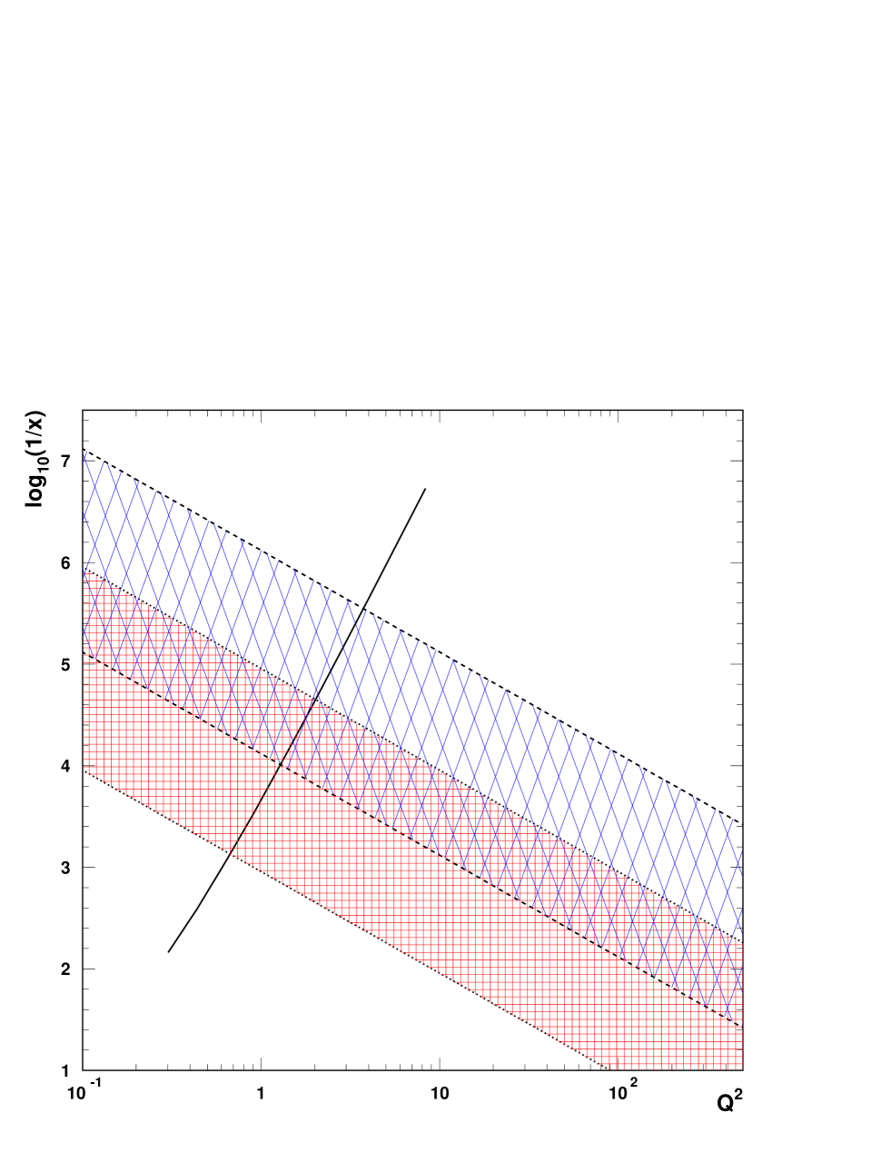
Figure 5: The position of the critical line in the $(x,Q^{2})$-plane. The narrow hatched area corresponds to the acceptance region of HERA. The wide hatched region indicates the range for a future $1~{}TeV$ $ep$-collider. The boundaries are lines of constant $y$.

In Fig. 5 we show the position of the critical line obtained in our analysis in the $(x,Q^{2})$ plane. We observe that going along the critical line from $x=10^{-4}$ to $x=10^{-5}$ we increase the saturation scale from approximately $1~{}GeV^{2}$ up to $2~{}GeV^{2}$. This means that even at a future $ep$-collider we expect only a rather small shift in the saturation scale. With great optimism it might go up to $3~{}GeV^{2}$ at a $1~{}TeV$ machine which, nevertheless, reaches quite far into the perturbative regime.

FIT RESULTS
	$\sigma_{0}$ (mb)	$~{}~{}~{}~{}\lambda~{}~{}~{}~{}$	$x_{0}$	$~{}~{}\chi^{2}/(no.exp.po.)~{}~{}$
no charm	23.03	0.288	$3.04\cdot 10^{-4}$	$441/372=1.18$
with charm	29.12	0.277	$0.41\cdot 10^{-4}$	$558/372=1.50$

An important prediction resulting from our analysis is the longitudinal structure function $F_{L}$ which is shown in Fig. 6. As we see $F_{L}$ constitutes roughly $20\%$ of $F_{2}$ for $Q^{2}$ around $10~{}GeV^{2}$ which is a reasonable value.

We now concentrate on the $W^{2}$ dependence of the total cross section $\sigma^{\gamma^{*}p}$ for fixed $Q^{2}$. We are particularly interested in the effective slope of $\sigma^{\gamma^{*}p}$ as a function of $W^{2}$. This dependence is shown in Fig. 7 in a broad range of $Q^{2}$ values and in Fig. 8 with a particular interest for smaller values of $Q^{2}<6.5~{}GeV^{2}$. Moving from high to low $Q^{2}$ we see how the slope of $\sigma^{\gamma^{*}p}$ flattens off indicating the low-$Q^{2}$ saturation. One can also recognize a slight curvature in particular for $Q^{2}=0$. This is associated with saturation in energy.

A more explicit way of exposing saturation is achieved by plotting the effective slope $\lambda_{eff}$ computed from the relation

$$\lambda_{eff}\;=\;\frac{\partial\ln(\sigma^{\gamma^{*}p})}{\partial\ln(W^{2})}$$ (30)

as a function of $Q^{2}$ for fixed values of $\tilde{x}=(Q^{2}+4m_{f}^{2})/(Q^{2}+W^{2})$. This means that we move along the dashed lines shown in Fig. 7 when computing the effective slope. The resulting curve is shown in Fig. 9. The transition from the “soft” to the “hard” regimes is clearly visible. Quite interestingly, $\lambda_{eff}$ at very low $Q^{2}$ turns out to be close to the standard value of $0.08$ for the soft Pomeron. This value is dependent on the choice of the quark mass which is not completely constrained. However, if the mass is chosen such that the cross section in the photoproduction region roughly agrees with the data it automatically leads to the right value for the slope in this region. The other important feature of small-$x$ saturation is that with decreasing $\tilde{x}$ the slope $\lambda_{eff}$ also decreases, as can be inferred from Fig. 9. In the true high energy asymptotics it would approach zero which is related to the fact that in the complex plane of angular momentum $j$ the leading singularity for our model is located at $j=1$.

3.2 Charm

Charm gives a substantial contribution to the total cross section $\sigma^{\gamma^{*}p}$ and cannot be ignored. We have performed a separate fit including charm but without introducing new parameters. Technically this means that in the basic formulae (2-4) the sum over flavours has to be extended to include charm with a mass of $1.5~{}GeV$. Also effected is $\tilde{x}$ in the corresponding dipole cross section (8,11) since it contains the quark mass (see eq. (20)). We do not change the light flavour mass and keep it equal to $140~{}MeV$. The impact of charm is shown in the second row of Table. 1 and in the last three plots. The $\chi^{2}$ of the fit has increased but is still acceptable. This is also reflected in Fig. 10 in which the agreement with the fitted data looks satisfactory. The most important change is a shift of the critical line down to smaller scales (see Fig. 10).

More visible is the effect of introducing charm in the $Q^{2}$-slope of $F_{2}$ shown in Fig. 11. The shape of the peak becomes broader and the value of the slope at the high end of $Q^{2}$ and $x$ increases. The main reason for broadening is the fact that charm saturates at a much higher scale due to its high mass. We also see that the critical line moves further away from the maxima. We still believe that the critical line characterizes the dynamical part of saturation in contrast to the saturation for charm which is entirely due to its small size and predominantly perturbative. But even a small size contribution will at extremely large $W^{2}$ be bigger than the saturation radius $R_{0}(x)$ and undergo small-$x$ saturation.

A rough comparison with preliminary data on the charmed structure function shows a reasonable agreement with the data at low $x$. We have again looked at the effective slope $\lambda_{eff}$, shown in Fig. 11, and find a slight increase at the low end of $Q^{2}$ of about $10\%$ as compared to our previous fit with light flavours only.

4 Implication on Diffraction

One of the important features of the wave function formalism is its flexible applicability for inclusive and diffractive scattering in DIS. We can immediately write down the cross section for diffractive scattering using the photon wave function defined in section 2 (see also ref.[18]):

$$\left.\frac{d\sigma_{T,L}^{D}}{dt}\right|_{t=0}\;=\;\frac{1}{16\pi}\;\int\!d\,^{2}{\bf r}\!\int_{0}^{1}\!dz\>|\Psi_{T,L}\,(z,{\bf r})|^{2}\>|\sigma\,(x,r^{2})|^{2}\;\\$$ (31)

and perform the Mellin transformation as in section 2.1

$$\left.\frac{d\sigma_{T,L}^{D}}{dt}\right|_{t=0} = \int\frac{d\nu}{2\pi}\int\!d\,^{2}{\bf r}\!\int_{0}^{1}\!dz\>|\Psi_{T,L}\,(z,{\bf r})|^{2}\>\int\frac{dr^{\prime 2}}{r^{\prime 2}}\left(\frac{r}{r^{\prime}}\right)^{1+2i\nu}|\sigma\,(\tilde{x},r^{\prime 2})|^{2}$$

$$= \sigma_{0}^{2}\;\;\int\frac{d\nu}{2\pi}\;\;\left[\left(\frac{x_{0}}{\tilde{x}}\right)^{\lambda}\frac{Q_{0}^{2}}{Q^{2}}\right]^{1/2+i\nu}\mbox{H${}_{T,L}$}\left(\nu,\frac{m_{f}^{2}}{Q^{2}}\right)\;\;\mbox{G}^{D}(\nu)\;\;.$$

The only change appears to be the function G${}^{D}(\nu)$. Provided the integrand in the second line of eq. (4) has at least a single pole at $\nu=-i/2$ we find the power behaviour with respect to the Bjorken variable $x$ to be the same for the inclusive as well as diffractive cross section. The explicit calculation of the function G^D defined by

$$\mbox{G}^{D}(\nu) = \int_{0}^{\infty}d\hat{r}^{2}\;\left(\hat{r}^{2}\right)^{-3/2-i\nu}\;\left(1\,-\,e^{-\hat{r}^{2}}\right)^{2}$$

$$= \;\left(2^{1/2+i\nu}-2\right)\;\Gamma(-1/2-i\nu)$$

$$= \left(2-2^{1/2+i\nu}\right)\mbox{G}(\nu)$$

reveals that G${}^{D}(\nu)$ is almost identical to G$(\nu)$ except for a factor which gives zero at $\nu=-i/2$. This zero has a common origin for all sensible models and simply reflects the fact that at small distances $r$ the cross section vanishes proportional to $r^{2}$ which in diffraction turns into $r^{4}$. In section 2.2, eq.(24), we found a double pole at $\nu=i/2$ in the integrand for the transverse part which is now reduced to a single pole. Since we are left with at least a single pole, the diffractive $\gamma p$-cross section for transverse polarized photons has indeed the same power behaviour in $x$ as the inclusive $\gamma p$-cross section.

We also found in section 2.2, eq.(25), that the inclusive longitudinal cross section had only a single pole which disappears completely in the diffractive cross section. The conclusion is that the next pole at $\nu=-3i/2$ becomes the leading pole and the power $1/2+i\nu$ in eq. (4) equals 2. Consequently, the longitudinal part in diffractive scattering rises at small $x$ two times as fast as in the inclusive case. Our result for the longitudinal contribution also confirms the well known higher twist nature of the diffractive cross section.

It is important to note that the results discussed in this section are derived without imposing cuts on the final state except for the basic rapidity cut. In particular, there has no cutoff being assumed for the transverse momentum of the final state partons. This allows to use formula (31). In ref. [22] a similar study lead to a closely related statement about the conservation of “anomalous dimensions”. In an extended version with non-zero momentum transfer links can be found to conformal invariance in the Regge limit [23].

We can go a step further and calculate the ratio of the diffractive and inclusive cross section in the limit of large $Q^{2}$. This can be done by shifting the contour of the $\nu$-integration down the lower half of the complex plane, as was done in section 2.3, and picking up the leading pole:

$$\frac{\sigma^{D}}{\sigma_{tot}}\;=\;\frac{\sigma_{0}}{4\pi B}\;\frac{3\;\ln(2)}{6\;\ln{Q^{2}}+6\;\lambda\;\ln(x/x_{0})+6\;\gamma_{E}+1}\;,$$ (34)

where $B$ denotes the diffractive slope. A mild logarithmic dependence on $x$ is found in the ratio which gives a slight logarithmic rise with decreasing $x$. Increasing $Q^{2}$ we find a logarithmic suppression which is due to the extra zero in G${}^{D}(\nu)$ at $\nu=-i/2$. Taking the parameters found in our fit and the experimental value for $B$ we find that the ratio turns out to be equal to a few percent. We have to note that a contribution of similar size is expected from the emission of a gluon. This contribution will have the same power behaviour in $x$ as for the quarks and we expect a ratio of a similar size. All contributions together will be of the order of 10%.

More precise studies on diffraction based on the model discussed here will be presented elsewhere [24].

5 Summary

We have presented a model which provides a good description of all DIS data below $x=0.01$ (including the photoproduction data). An important ingredient of our approach is the presence of small-$x$ saturation. This is achieved by introducing an $x$-dependent saturation radius $R_{0}(x)=(x/x_{0})^{\lambda/2}$ which we define with the help of two parameters. These parameters, together with the overall normalization of the cross section, was determined by fits to the DIS data. The parameterization obtained in this way was then extended into the photoproduction region showing reasonable agreement with the data there. A particular result of this extrapolation is the effective Pomeron intercept of approximately $1.08$. In the DIS region this effective intercept increases to the asymptotical value of $1.29$. We have introduced a “critical line” which marks the boundary of the saturation region in the $(x,Q^{2})$-plane. Finally, we found an intriguing result when applying our model to diffractive scattering processes, namely, an almost constant ratio of diffractive and inclusive DIS cross section.

Our model is basically phenomenological. It is remarkable, however, that with only three fitted parameters we successfully described the small-$x$ data. The theoretical basis is the separation of the perturbative dissociation of the photon into a quark-antiquark pair and the subsequent interaction of the pair with the proton. The latter is modelled in an eikonal way. The main consequence is that we do not only have saturation at low $Q^{2}$, but also saturation at low $x$. The natural extension of our model would be the incorporation of a perturbative treatment for large $Q^{2}$. Also important is the development of a microscopical picture behind saturation as proposed in ref.[25].

A real test for our model would by a future $ep$-collider. Our prediction is that with increasing energy the saturation scale moves up in $Q^{2}$. For an $1~{}TeV$ collider it woud be roughly a factor of $2$.

Acknowledgements

We thank Alan Martin, Jan Kwiecinski and Misha Ryskin for valuable discussions. KG-B thanks the Royal Society/NATO for financial support and the Department of Physics of the University of Durham for warm hospitality. This research has been supported in part the Polish State Committee for Scientific Research grant no. 2 P03B 089 13 and by the EU Fourth Framework Programme “Training and Mobility of Researchers” Network, “Quantum Chromodynamics and the Deep Structure of Elementary Particles”, contract FMRX-CT98-0194 (DG 12-MIHT).

Figure 3: The $\gamma^{*}p$-cross section for various energies. The solid lines show the fit results with a light quark mass of 140MeV. The dotted lines show the cross section with the same parameters but with zero quark mass. The line across the curves indicates the position of the critical line.

Figure 4: The logarithmic $Q^{2}$-slope of $F_{2}$ for fixed energies $W$, plotted as a function of $Q^{2}$ and $x$. The line across the curves shows the position of the critical line.

Figure 6: $F_{2}$ and $F_{L}$ structure functions plotted as a function of $Q^{2}$ for fixed energies $W$.

Figure 7: The total $\gamma^{*}p$-cross section as a function of $W^{2}$ for different $Q^{2}$-values. The dashed lines represent the lines of constant $\tilde{x}$ as defined in eq.(20).

Figure 8: The same cross section as in Fig. 7 with the emphasis on small-$Q^{2}$ values.

Figure 9: The effective slope in $W^{2}$ of the total cross section, $\lambda_{eff}$, plotted as a function of $Q^{2}$ for fixed $\tilde{x}$. The solid line appears twofold due to two different methods of calculation. One is based on the analytical expression (30), the second is calculated from fig.7 by taking a pair of points along the lines of constant $\tilde{x}=10^{-2}$ and $10^{-4}$.

Figure 10: The $\gamma^{*}p$-cross section including charm. The charm contribution itself is plotted as dotted line.

Figure 11: The logarithmic $Q^{2}$-slope of $F_{2}$ with charm. The dashed line shows the charm contribution.

Figure 12: The effective slope $\lambda_{eff}$ based on the charm fit. The intercept is slightly higher at low $Q^{2}$ as compared to fig.9.

References

- [1] L.V.Gribov, E.M.Levin, M.G.Ryskin, Phys. Rep. 100 (1983) 1.
- [2] J.Bartels, Phys. Lett. B298 (1993) 204.
- [3] A.H.Mueller, Nucl. Phys. B335 (1990) 115.
- [4] N.Nikolaev, B.G.Zakharov, Z. Phys. C49 (1990) 607.
- [5] N.Nikolaev, E.Predazzi, B.G.Zakharov, Phys. Lett. B326 (1994) 161.
- [6] E.Gotsman, E.Levin, U.Maor, Phys. Lett. B425 (1998) 369.
- [7] W.Buchmüller, A.Hebecker, Nucl. Phys. B476 (1996) 203; W.Buchmüller, A.Hebecker, M.F.Mc Dermott, Nucl. Phys. B487 (1997) 283.
- [8] J.R. Forshaw and D.A. Ross, QCD and the Pomeron, Cambridge University Press, 1986.
- [9] H1 collaboration, Nucl. Phys. B497 (1997) 3; Nucl. Phys. B470 (1996) 3.
- [10] ZEUS collaboration, Phys. Lett. B407 (1997) 432; Z. Phys. C69 (1996) 607.
- [11] B.Badelek, J.Kwiecinski, Phys. Lett. B295 (1992) 263.
- [12] A.Martin, M.G.Ryskin, A.M.Stasto, preprint DTP/98/20, hep-ph/9806212.
- [13] A.Donnachie, P.V.Landshoff, preprint DAMPT-1998-34, hep-ph/9806344.
- [14] M.Rueter, preprint TAUP-2507-98, hep-ph/9807448.
- [15] A.B.Kaidalov, C.Merino. hep-ph/9806367
- [16] D.Schildknecht, H.Spiesberger, preprint BI-TP-97-25, hep-ph/9707447.
- [17] W.Buchmüller, D.Haidt, preprint DESY-96-061, hep-ph/9605428.
- [18] N.N. Nikolaev, B.G. Zakharov, Z. Phys. C53 (1992) 331.
- [19] A.L.Ayala Filho, M.B.Gay Ducati, E.M.Levin, Nucl.Phys. B511 (1998) 355.
- [20] ZEUS collaboration, XXIX International Conference on High Energy Physics, Vancouver, July 23-29, 1998.
- [21] H.Abramowicz, A.Levy, preprint DESY-97-251, hep-ph/9712415.
- [22] J.Bartels, H.Lotter, M.Wüsthoff, Z. Phys. C68 (1995) 121.
- [23] J.Bartels, L.Lipatov, M.Wüsthoff, Nucl. Phys. B464 (1996) 298.
- [24] K.J.Golec-Biernat, M.Wüsthoff, paper in preparation.
- [25] J.Jalilian-Marian, A.Kovner, A.Leonidov, H.Weigert, preprint Cavendish-HEP-98/12, hep-ph/9807462.