DTP/98/48

July 1998

Off-diagonal parton distributions and their evolution

K.J. Golec-Biernat and A.D. Martin

Department of Physics, University of Durham, Durham, DH1 3LE, UK.

We construct off-diagonal parton distributions defined on the interval $0\leq X\leq 1$ starting from the off-forward distributions defined by Ji. We emphasize the particular role played by the symmetry relations in the “ERBL-like” region. We find the evolution equations for the off-diagonal distributions which conserve these symmetries. We present numerical results of the evolution, and verify that the analytic asymptotic forms of the parton distributions are reproduced. We also compare the constructed off-diagonal distributions with the non-forward distributions defined by Radyushkin and comment on the singularity structure of the basic amplitude written in terms of the off-diagonal distributions.

1 Introduction

It is well known that the cross section of hard scattering processes (such as deep inelastic scattering, the production of large $p_{T}$ jets, etc.) can be written as the sum of parton distributions multiplied by the cross sections of hard subprocesses calculated at the parton level using perturbative QCD. That is we can factor off the long distance (non-perturbative) effects into universal, process independent, parton distributions ($f_{i}(X,\mu^{2})$ with $i=q,\bar{q},g$) specific to the incoming hadrons. $X$ is the longitudinal fraction of the hadron’s momentum that is carried by the parton and $\mu$ is a scale typical of the hard subprocess. The parton distributions are given by the matrix elements $\langle P|\hat{O}|P\rangle$ where $\hat{O}$ is a twist-2 quark or gluon operator, and $P$ represents the full set of quantum numbers of the hadron. To be specific we will be concerned with a proton taking part in unpolarised reactions. Thus $P$ will represent the 4-momentum of the proton.

Calculating the parton distributions from first principles is one of the most challenging problems in non-perturbative QCD. The most promising approach is lattice QCD, but much remains to be done. On the other hand, from a practical viewpoint, the parton distributions of the proton are determined with good precision from global analyses of deep inelastic and related hard scattering data. The distributions $f_{i}(X,\mu^{2})$ are parametrized as a function of $X$ at some starting scale $\mu_{0}^{2}$ and then evolved using the DGLAP equations of perturbative QCD to higher $\mu^{2}$ values relevant to the data to be fitted.

Recently [1]–[9] there has been much interest in off-diagonal (also called off-forward by Ji [1] or non-forward by Radyushkin [4]) distributions which are given by matrix elements $\langle P^{\prime}|\hat{O}|P\rangle$ in which the momentum of the outgoing proton is not the same as that of the incoming proton. For example, the amplitudes for processes such as deeply virtual Compton scattering $(\gamma^{*}p\rightarrow\gamma p)$ or vector particle electroproduction $(\gamma^{*}p\rightarrow Zp$ or $J/\psi p$) depend on off-diagonal distributions. Since $P\neq P^{\prime}$ the parton returning to the proton has a different momentum to the one which is outgoing, and so we need two momentum variables to specify the off-diagonal distributions. The Ji and Radyushkin distributions, which are denoted by $H(x,\xi)$ and ${\cal{F}}_{\zeta}(X)$ respectively, differ in their choice of the defining four vector. Ji chooses the momentum fractions $x$ and $\xi$ with respect to the average of the incoming and outgoing proton momenta $\bar{P}=\frac{1}{2}(P+P^{\prime})$, whereas Radyushkin defines $X$ and $\zeta$ with respect to the incoming proton momentum $P$. The former has the important advantage that it is easier to impose the symmetry requirements, while the latter has the advantage that it is close to the definition used for the conventional (diagonal) distributions. Our aim is to clarify the relation between the two formulations. We find that they are not equivalent unless specific conditions are imposed on Radyushkin’s non-forward distributions. We show this by a direct construction of distributions defined in the range $0\leq X\leq 1$ which are equivalent to Ji’s off-forward distributions.

Let us neglect, for the moment, the gluon distribution. The quark distribution $H_{q}(x,\xi)$, defined by Ji, covers the interval $-1\leq x\leq 1$ and generates two distinct distributions which we denote by $\hat{\cal{F}}_{q}(X,\zeta)$ and $\hat{\cal{F}}_{\bar{q}}(X,\zeta)$ with $0\leq X\leq 1$. Over the region $X>\zeta$ the two functions $\hat{\cal{F}}_{q}$ and $\hat{\cal{F}}_{\bar{q}}$ are independent. On the other hand in the region $X<\zeta$ they are related to each other, with the consequence that the non-singlet and singlet combinations possess a symmetry about $X=\zeta/2$. We obtain evolution equations for $\hat{\cal{F}}$ starting from the evolution equations for the off-forward distributions $H$. We find that they differ from the evolution equations for the non-forward distributions [5, 9] by additional terms which are essential to preserve the symmetry properties in the ERBL-like region. We also found that the basic amplitude for deeply virtual Compton scattering (DVCS) has a different singularity structure to that given by the non-forward distributions ${\cal{F}}$.

The outline of the paper is as follows. To establish notation we quickly review in Section 2 the salient features of the conventional (diagonal) parton distributions $H(x)$ with support $-1\leq x\leq 1$. Section 3 reviews the extension of these ideas to the off-diagonal distributions $H(x,\xi)$ that were introduced by Ji [1]. In Section 4 we transform the distributions $H(x,\xi)$ into distributions $\hat{\cal{F}}(X,\zeta)$ with $0\leq X\leq 1$, and demonstrate that $\hat{\cal{F}}$ must satisfy symmetry relations for $X<\zeta$. In Section 5 we give the evolution equations for the $\hat{\cal{F}}(X,\zeta)$ and present numerical solutions. The complete form of the evolution equations is given in the Appendix. In Section 6 we discuss the relation between the distributions $\hat{\cal{F}}$ and the non-forward distributions ${\cal{F}}$ of Radyushkin. In the same spirit we discuss the differences in the singularity structure of the DVCS amplitude. Finally Section 7 contains our conclusions.

2 Conventional parton distributions

In order to introduce off-diagonal distributions it is most convenient to first recall the definition of the conventional (diagonal) parton distributions in terms of light-cone coordinates $(x^{\pm}=(x^{0}\pm x^{3})/\sqrt{2},x^{1},x^{2})$ and in the light-cone gauge $(A^{+}=0)$ [10]. For instance the quark distribution $H_{q}(x)$ is given in terms of the matrix element of a light-cone bilocal operator

$$H_{q}(x)\;=\;\frac{1}{2}\int\frac{dy^{-}}{2\pi}e^{-ixP^{+}y^{-}}\>\langle P|\bar{\psi}_{q}\!(0,y^{-}/2,\mbox{\boldmath$0$})\>\textstyle{\frac{1}{2}}\gamma^{+}\>\psi_{q}\!\left(0,-y^{-}/2,\mbox{\boldmath$0$}\right)|P\rangle.$$ (1)

Note that the matrix element is diagonal in the four momentum $P$ of the proton. For simplicity we do not show either here, or throughout the paper, the renormalization scale dependence of $H_{q}$ and of the other parton distributions that we discuss.

To see the parton content of the distribution $H_{q}$ we make a Fourier expansion of (the light-cone-plus or ‘good’ component) $\psi_{+}$ of the quark field, in terms of the quark annihilation operator $b$ and the antiquark creation operator $d^{\dagger}$. Similarly $\bar{\psi}_{+}$ is expanded in terms of $b^{\dagger}$ and $d$, and then the integration over $y^{-}$ in (1) is performed. It is found that $H_{q}$ is only non-vanishing in the interval $-1\leq x\leq 1$ with the term $b^{\dagger}b$ contributing for $x>0$ and $dd^{\dagger}$ contributing for $x<0$ [11]

$$H_{q}(x) = \frac{1}{2P^{+}}\>\int\>\frac{d^{2}k_{T}}{2x(2\pi)^{3}}\>\sum_{\lambda}\left[\langle P|b_{\lambda}^{\dagger}\!(xP^{+},\mbox{\boldmath$k$}_{T})\>b_{\lambda}\!(xP^{+},\mbox{\boldmath$k$}_{T})|P\rangle\>\theta(x)\right.$$

$$-\!\left.\langle P|d_{\lambda}^{\dagger}\!(-xP^{+},\mbox{\boldmath$k$}_{T})\>d_{\lambda}\!(-xP^{+},\mbox{\boldmath$k$}_{T})|P\rangle\>\theta(-x)\;,\right]$$

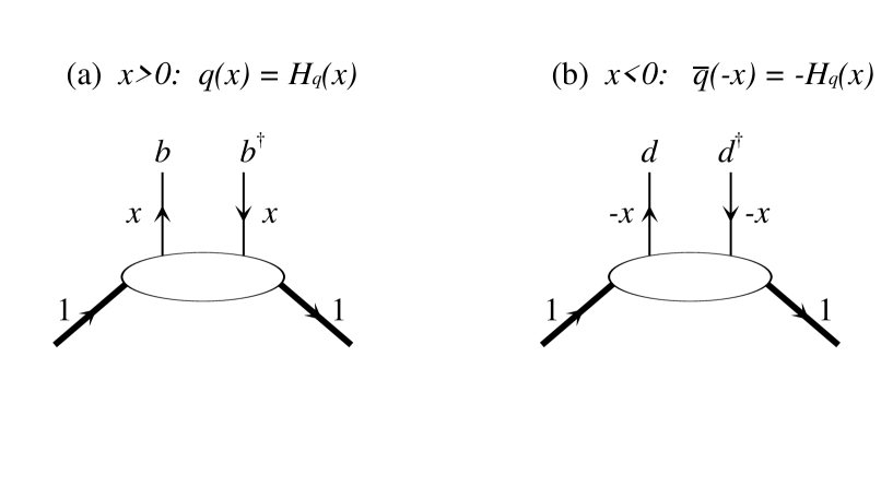
Figure 1: Schematic diagrams showing the contributions to $H_{q}(x)$ with $x>0$ and $x<0$ respectively, which can be identified with the familiar quark and antiquark distributions. $b,b^{\dagger}$ are the quark annihilation and creation operators and $d,d^{\dagger}$ are those for the antiquark. The momentum fractions refer to the plus light-cone component of the incoming proton momentum $P$.

where $\lambda$ is the helicity of the quarks. The $b^{\dagger}b$ term corresponds to the emission of a quark (carrying a fraction $x$ of the proton’s momentum) and its subsequent reabsorption within the proton. Similarly the $d^{\dagger}d$ contribution describes the emission and subsequent reabsorption of an antiquark. The two possibilities are sketched in Fig. 1. Thus the single distribution $H_{q}$ with support in the interval $-1\leq x\leq 1$ embodies both the familiar $q$ and $\bar{q}$ distributions, defined on the interval $0\leq x\leq 1$, which thus are identified with the two terms accompanying the theta functions in (2) in the following way

$$H_{q}(x)\;=\>\left\{\begin{array}[]{lcl}q(x)&{\rm for}&x>0\\ &&\\ -\bar{q}(-x)&{\rm for}&x<0.\end{array}\right.$$ (3)

We may form the valence and singlet quark distributions in terms of $H_{q}$

$$q(x)\;-\;\bar{q}(x) = H_{q}(x)\;+\;H_{q}(-x)\;\equiv\;H_{q}^{V}(x)$$

$$\sum_{q}\>\left[q(x)\;+\;\bar{q}(x)\right] = \sum_{q}\left[H_{q}(x)\>-\>H_{q}(-x)\right]\;\equiv\;H^{S}(x)\;,$$

where the sum is over the quark flavours. Clearly over the full interval $-1\leq x\leq 1$ the valence and singlet quark distributions satisfy the symmetry relations

$$H_{q}^{V}(x) = H_{q}^{V}(-x)$$

$$H^{S}(x) = -H^{S}(-x)\;.$$

In a similar way we may introduce $H_{g}(x)\equiv xg(x)$ where $g(x)$ is the familiar gluon distribution. In the light-cone gauge

$$H_{g}(x)\;=\;\frac{1}{P^{+}}\>\int\>\frac{dy^{-}}{2\pi}\>e^{-ixP^{+}y^{-}}\>\langle P|F^{+\nu}(0,y^{-},\mbox{\boldmath$0$})\>F_{\nu}^{+}(0,0,\mbox{\boldmath$0$})|P\rangle\;,$$ (6)

where $F^{\mu\nu}$ is the gluon field strength tensor and where the summation over the colour label has been suppressed. Due to Bose symmetry we have

$$H_{g}(x)\;=\;H_{g}(-x)\;.$$ (7)

3 Off-diagonal distributions

The distributions $H_{q}$ introduced in (1) may be generalized to allow for matrix elements which are off-diagonal in the four momentum of the proton [1]–[3]

$$H_{q}(x,\xi,t)\;=\;\frac{1}{2}\>\int\>\frac{dy^{-}}{2\pi}\>e^{-ix{\bar{P}}^{+}y^{-}}\>\langle P^{\prime}|\bar{\psi}_{q}(0,y^{-}/2,\mbox{\boldmath$0$})\>\textstyle{\frac{1}{2}}\gamma^{+}\psi_{q}(0,-y^{-}/2,\mbox{\boldmath$0$})|P\rangle\;,$$ (8)

where we consider only the distributions which conserve the proton helicity and which describe unpolarized quarks. Since $\Delta\equiv P-P^{\prime}\neq 0$ the distribution $H_{q}(x,\xi,t)$ now contains two extra scalar variables, in addition to the Bjorken $x$ variable. The variable $t$ is the usual $t$-channel invariant, $t=\Delta^{2}$, and the variable $\xi$ is defined by

$$\xi\bar{P}^{+}\;=\;\frac{1}{2}\Delta^{+}\;,$$ (9)

where $\bar{P}=\frac{1}{2}(P+P^{\prime})$. This choice of variables is due to Ji [1]–[3] and enables symmetry to be imposed between the incoming and outgoing proton. That is Ji uses the symmetric combination $\bar{P}$ of their momenta as the defining direction, and calls the $H_{q}$ off-forward distributions. The distributions $H_{q}$ are real, and the symmetric choice of variables has the considerable advantage that, due to time-reversal invariance and hermiticity, the distributions are even functions of $\xi$ [3]

$$H_{q}(x,\xi,t)\;=\;H_{q}(x,-\xi,t)\;.$$ (10)

Since we will perform our analysis for fixed $t$, concentrating on the $x$ and $\xi$ dependence, we shall omit the $t$ dependence from now on.

To see the physical content of the off-diagonal distributions $H_{q}$ we again Fourier expand $\psi$ and $\bar{\psi}$ in terms of the quark creation and annihilation operators. Since the distributions are even in $\xi$ we may take $\xi>0$. In this way we obtain the generalization of eq. (2) [3]

$$H_{q}(x,\xi) = \frac{1}{2\bar{P}^{+}}\int\frac{d^{2}k_{T}}{2\sqrt{|x^{2}-\xi^{2}|}(2\pi)^{3}}$$

$$\sum_{\lambda}\left[\langle P^{\prime}|b_{\lambda}^{\dagger}\,((x-\xi)\bar{P}^{+},\mbox{\boldmath$k$}_{T}-\mbox{\boldmath$\Delta$}_{T})\>b_{\lambda}\,((x+\xi)\bar{P}^{+},\mbox{\boldmath$k$}_{T})|P\rangle\>\theta(x\geq\xi)\right.$$

$$+\;\langle P^{\prime}|d_{\lambda}\,((-x+\xi)\bar{P}^{+},-\mbox{\boldmath$k$}_{T}+\mbox{\boldmath$\Delta$}_{T})\>b_{-\lambda}\,((x+\xi)\bar{P}^{+},\mbox{\boldmath$k$}_{T})|P\rangle\>\theta(-\xi<x<\xi)$$

$$-\;\left.\langle P^{\prime}|d_{\lambda}^{\dagger}\,((-x-\xi)\bar{P}^{+},\mbox{\boldmath$k$}_{T}-\mbox{\boldmath$\Delta$}_{T})\>d_{\lambda}\,((-x+\xi)\bar{P}^{+},\mbox{\boldmath$k$}_{T})|P\rangle\>\theta(x\leq-\xi)\right].$$

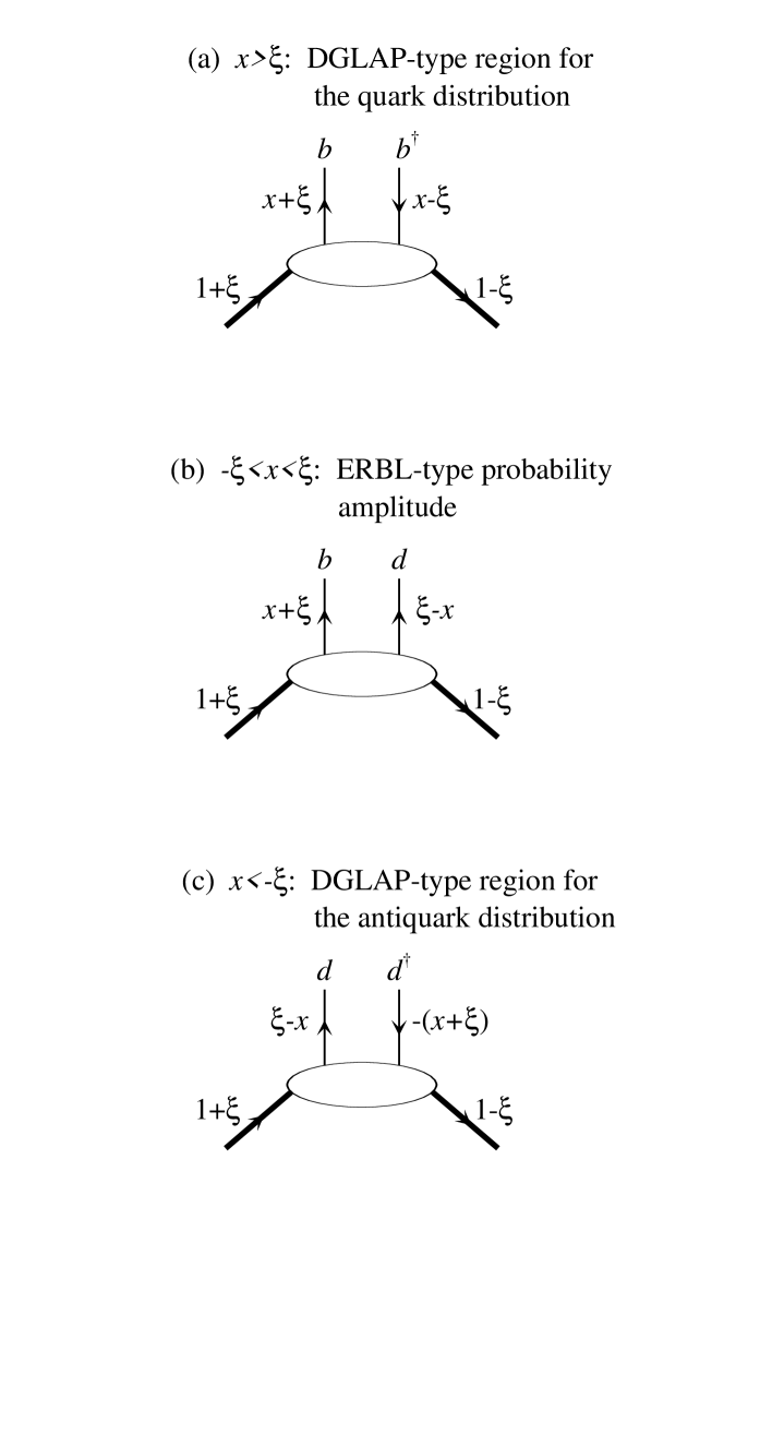
Figure 2: Schematic diagrams of the off-diagonal distribution $H_{q}(x,\xi)$, in the three distinct kinematic regions. The proton and quark momentum fractions refer to $\bar{P}^{+}$, where $\bar{P}$ is the average of the incoming and outgoing proton four momentum. Note that the four momentum transfer satisfies $\Delta^{+}=2\xi\bar{P}^{+}$ and that $x$ covers the interval $[-1,1]$.

Fig. 2 gives a pictorial description of the content of (3). Diagrams (a) and (c), which arise from the $b^{\dagger}b$ and $d^{\dagger}d$ terms in $\bar{\psi}\psi$, generalize Figs. 1(a) and (b) respectively. For example the first diagram corresponds to the emission of a quark of momentum $k$ from the proton followed by its absorption with momentum $k-\Delta$. Thus for $x>\xi$ and $x<-\xi$ the off-diagonal distribution $H_{q}$ generalizes the familiar quark and antiquark distributions and will evolve according to modified DGLAP equations. Diagram (b), corresponding to the middle region, $-\xi<x<\xi$, does not have a counterpart in Fig. 1. This diagram, which arises from the $db$ term in $\bar{\psi}\psi$, corresponds to the emission of a quark-antiquark pair. In this region $H_{q}$ is a generalization of the proton form factor and will evolve according to modified ERBL equations [12]. Thus in this domain $H_{q}$ may be regarded as a generalization of the probability distribution amplitude which occurs in hard exclusive processes.

Just as for the diagonal case, we introduce valence and singlet quark distributions analogous to (2)

$$H_{q}^{V}(x,\xi)\equiv H_{q}(x,\xi)\>+\>H_{q}(-x,\xi)\;=\;H_{q}^{V}(-x,\xi)\;,$$ (12)

$$H^{S}(x,\xi)\equiv\sum_{q}\left[H_{q}(x,\xi)\>-\>H_{q}(-x,\xi)\right]\;=\;-H^{S}(-x,\xi)\;.$$ (13)

Thus in addition to the symmetry under $\xi\rightarrow-\xi$, the distributions have symmetry or antisymmetry under $x\rightarrow-x$. Also, in analogy to (7), the off-diagonal gluon distribution satisfies

$$H_{g}(x,\xi)\;=\;H_{g}(-x,\xi)\;.$$ (14)

The distributions (12)-(14) are identical to those introduced by Ji [2, 3] except that

$$H_{g}(x,\xi)\;=\;xH_{g}^{\rm Ji}(x,\xi).$$ (15)

On account of the extra factor $x$, the gluon distribution (15) is not required to be zero at $x=0$, unlike the situation for $H_{g}^{\rm Ji}$ (see also [5] for a relevant discussion).

4 Off-diagonal distributions on the interval $[0,1]$

So far we have considered the off-diagonal distributions $H_{q}(x,\xi)$, introduced by Ji [1, 2], and defined on the interval $-1<x<1$. As noted above $P+P^{\prime}$ is taken as the defining direction, so that symmetry is imposed between the incoming $(P)$ and outgoing $(P^{\prime})$ proton momenta. This variable $\xi$ was defined in (9) by

$$\Delta\;\equiv\;(P-P^{\prime})\;=\;\xi(P+P^{\prime})\;,$$ (16)

where for simplicity we have omitted the light-cone plus superscript (see (9)).

To make direct contact with conventional partons we may introduce alternative off-diagonal distributions $\hat{\cal{F}}_{q}(X,\zeta)$ defined on the interval $0\leq X\leq 1$ such that the initial parton carries a positive fraction $X$ of the proton’s longitudinal momentum. That is we take $P$ as the defining direction. Thus the counterpart to (16) is

$$\Delta\;=\;\zeta P$$ (17)

with $0\leq\zeta\leq 1$. This is exactly analogous to the approach introduced by Radyushkin [4, 5] in the construction of the non-forward distributions ${\cal{F}}_{\zeta}(X)$. However our construction of the distributions $\hat{\cal{F}}_{q}(X,\zeta)$ presented below is different to that of [4, 5]. From (16) and (17) it follows that

$$\xi\;=\;\frac{\zeta}{2-\zeta}\;.$$ (18)

4.1 The relation between the distributions $H$ and $\hat{\cal{F}}$

In this subsection we first define the off-diagonal distributions $\hat{\cal{F}}_{q}(X,\zeta)$ with $X$ in the interval [0,1] starting from Ji’s distributions $H_{q}(x,\xi)$ with $x$ in the range [-1,1]. Then we explore the symmetry relations satisfied by the $\hat{\cal{F}}_{q}(X,\zeta)$.

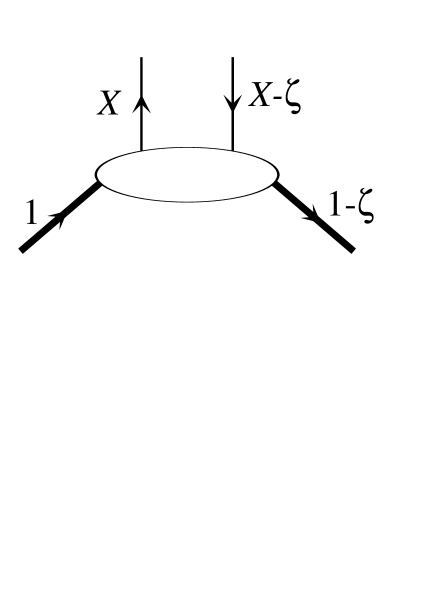
Figure 3: The proton and quark momentum fractions with respect to the initial proton momentum $P$ corresponding to the off-diagonal distributions $\hat{\cal{F}}(X,\zeta)$ defined in the domain $0\leq~{}X\leq~{}1$. The four momentum transfer satisfies $\Delta^{+}=\zeta P^{+}$.

If we compare the momentum fraction carried by the emitted parton in Fig. 3 with those in Figs. 2(a) and 2(c), then we see that two different transformations are relevant in reducing the interval $-1\leq x\leq 1$ covered by $H_{q}(x,\xi)$ to the interval $0\leq X\leq 1$ covered by $\hat{\cal{F}}_{q}(X,\zeta)$. First, from Fig. 2(a), we have the transformation

$$X_{1}\;=\;\frac{x_{1}+\xi}{1+\xi}\;,$$ (19)

which takes the interval $x_{1}\in[-\xi,1]$ into $X_{1}\in[0,1]$. Simultaneously $\xi$ is transformed into $\zeta$. Secondly, from Fig. 2(c), we have the transformation

$$X_{2}\;=\;\frac{\xi-x_{2}}{1+\xi}\;,$$ (20)

which takes $x_{2}\in[-1,\xi]$ into $X_{2}\in[0,1]$. Now, $-\xi$ is transformed into $\zeta$. In this way we introduce two distinct off-diagonal distributions $\hat{\cal{F}}_{q}$ and

$$\hat{\cal{F}}_{q}(X_{1},\zeta) = \frac{1}{1-\zeta/2}\;H_{q}(x_{1},\xi)$$

$$\hat{\cal{F}}_{\bar{q}}(X_{2},\zeta) = \frac{-1}{1-\zeta/2}\;H_{q}(x_{2},\xi)\;,$$

where $\xi=\zeta/(2-\zeta)$ and the inverse relations

$$x_{1}\;=\;\frac{X_{1}-\zeta/2}{1-\zeta/2}\;,\quad\quad\quad x_{2}\;=\;\frac{\zeta/2-X_{2}}{1-\zeta/2}$$ (22)

follow from (18–20). We stress that as $X_{1,2}$ cover the range $[0,1]$, the corresponding $x_{1}$ and $x_{2}$ cover respectively the ranges $[-\xi,1]$ and $[-1,\xi]$, as shown schematically in Fig. 4. The factors $\pm(1-\zeta/2)^{-1}$ in (4.1) arise from the translation of the measure $dx$ to $dX$.

In the limit that $\zeta$ (and $\xi$) $\rightarrow 0$ we have from (3)

$$\hat{\cal{F}}_{q}(X,0) = ~{}~{}~{}~{}H_{q}(X,0)\;=\;q(X)$$

$$\hat{\cal{F}}_{\bar{q}}(X,0) = -H_{q}(-X,0)\;=\;\bar{q}(X)\;,$$

which is an additional motivation for using the quark and antiquark subscripts to differentiate between the two functions $\hat{\cal{F}}_{q}$ and $\hat{\cal{F}}_{\bar{q}}$.

Finally, due to the symmetry relation (14), the gluon distribution may be defined in the range $0\leq X\leq 1$ by either of the transformations (22). That is we have

$$\hat{\cal{F}}_{g}(X,\zeta)\;=\;\frac{1}{1-\zeta/2}\>H_{g}\left(\frac{X-\zeta/2}{1-\zeta/2},\xi\right)\;=\;\frac{1}{1-\zeta/2}\>H_{g}\left(\frac{\zeta/2-X}{1-\zeta/2},\xi\right).$$ (24)

4.2 Symmetry relations

From Fig. 4 we see that in the DGLAP-type regions ($x>\xi$ or $x<-\xi$) $H_{q}$ is transformed respectively into independent functions $\hat{\cal{F}}_{q}(X)$ and $\hat{\cal{F}}_{\bar{q}}(X)$ with $X>\zeta$. On the other hand in the ERBL-type region ($-\xi<x<\xi$) the distribution $H_{q}$ generates functions $\hat{\cal{F}}_{q}(X)$ and $\hat{\cal{F}}_{\bar{q}}(X)$ with $X<\zeta$ which are no longer independent. Indeed for $X<\zeta$ we have

$$\hat{\cal{F}}_{q}(\zeta-X) = \frac{1}{1-\zeta/2}\>H_{q}\left(\frac{\zeta-X-\zeta/2}{1-\zeta/2}\right)\;=\;\frac{1}{1-\zeta/2}\;H_{q}\left(\frac{\zeta/2-X}{1-\zeta/2}\right)$$ (25)

$$= \;-\hat{\cal{F}}_{\bar{q}}(X)\;,$$

where for simplicity we do not indicate the additional explicit $\zeta$ or $\xi$ dependence of the distributions.

Eq. (25) is the basic symmetry relation for the off-diagonal quark distributions which indicates that in the ERBL-like region the quark and antiquark distributions are not independent, unlike the case in the DGLAP-like region. The physical reason for this can easily be understood by looking at Fig. 2b. In the ERBL-like region we can define the off-diagonal distributions with respect to the first emitted parton being either the quark with momentum $x+\xi$ or the antiquark with momentum $\xi-x$. The latter possibility corresponds to the exchange of the annihilation operators in eq. (3), which is the origin of the $-$ sign in relation (25).

We may form the non-singlet and singlet combinations of the quark and antiquark distributions. From (12) we have

$$\hat{\cal{F}}_{q}^{V}(X) = \frac{1}{1-\zeta/2}\;H_{q}^{V}\left(\frac{X-\zeta/2}{1-\zeta/2}\right)\;=\;\hat{\cal{F}}_{q}(X)-\hat{\cal{F}}_{\bar{q}}(X)\;,$$

$$\hat{\cal{F}}^{S}(X) = \frac{1}{1-\zeta/2}\;H^{S}\left(\frac{X-\zeta/2}{1-\zeta/2}\right)\;=\;\sum_{q}\left[\hat{\cal{F}}_{q}(X)+\hat{\cal{F}}_{\bar{q}}(X)\right]\;,$$

which in the region $X<\zeta$ satisfy symmetry relations resulting from (25)

$$\hat{\cal{F}}_{q}^{V}(\zeta-X) = \hat{\cal{F}}_{q}^{V}(X)\;,$$

$$\hat{\cal{F}}^{S}(\zeta-X) = -\hat{\cal{F}}^{S}(X)\;.$$

It is straightforward to show for $X<\zeta$ that the gluon distribution (24) satisfies a similar relation

$$\hat{\cal{F}}_{g}(\zeta-X)\;=\;\hat{\cal{F}}_{g}(X)\;.$$ (28)

These properties are well-illustrated by Fig. 5. The upper plot shows an example of the off-diagonal distribution $H_{q}(x,\xi)$ with $x\in[-1,1]$, for $\xi=0.5$. The middle plot shows the transformation of this distribution into the two functions $\hat{\cal{F}}_{q}(X,\zeta)$ and $\hat{\cal{F}}_{\bar{q}}(X,\zeta)$ of (4.1) with $X\in[0,1]$. Their behaviour shows that the symmetry relation (25) is clearly satisfied in the region $0\leq X\leq\zeta$. Finally, the lower plot shows the behaviour of the non-singlet $\hat{\cal{F}}_{q}^{V}$ and the singlet $\hat{\cal{F}}^{S}$ combinations. The symmetry of $\hat{\cal{F}}_{q}^{V}$ and antisymmetry of $\hat{\cal{F}}^{S}$, about the point $X=\zeta/2$, are clearly evident in the region $0\leq X\leq\zeta$.

5 Evolution equations

Just as we constructed $\hat{\cal{F}}$ directly from the off-forward distributions $H$ of Ji, so we start with the evolution equations [2] for $H(x,\xi)$ with $x\in[-1,1]$ and use transformations (4.1) and (24) to rewrite them in terms of the distributions $\hat{\cal{F}}(X,\zeta)$ with $X\in[0,1]$.

In the DGLAP-like region $X>\zeta$ (which corresponds to $x>\xi$ or $x<-\xi$) the equations that we obtain for $\hat{\cal{F}}$ are equivalent to those given for the non-forward distributions of Radyushkin [5, 9]. Their full form can be found in the Appendix. Moreover in the limit $\zeta\rightarrow 0$ they reduce to the familiar DGLAP evolution equations.

However in the ERBL-like region $X<\zeta$ (corresponding to $-\xi<x<\xi$) the equations obtained for $\hat{\cal{F}}$ are different to those given in [5, 9] for the non- forward distributions. They have the following forms

$$\mu\frac{\partial}{\partial\mu}\>\hat{\cal{F}}_{q}^{V}(X,\zeta) = P_{QQ}\otimes\hat{\cal{F}}_{q}^{V}$$ (29)

$$+ \frac{\alpha_{S}C_{F}}{\pi}\int_{\zeta}^{1}\frac{dZ}{Z}\!\left[\frac{Z}{X-\zeta+Z}-\frac{X}{\zeta}\right]\>\hat{\cal{F}}_{q}^{V}(Z,\zeta)$$

$$\mu\frac{\partial}{\partial\mu}\hat{\cal{F}}^{S}(X,\zeta) = P_{QQ}\otimes\hat{\cal{F}}^{S}\>+\>P_{QG}\otimes\hat{\cal{F}}_{g}$$

$$- \frac{\alpha_{S}C_{F}}{\pi}\int_{\zeta}^{1}\frac{dZ}{Z}\!\left[\frac{Z}{X-\zeta+Z}-\frac{X}{\zeta}\right]\>\hat{\cal{F}}^{S}(Z,\zeta)$$

$$+ \>\frac{\alpha_{S}N_{f}}{\pi}\int_{\zeta}^{1}\frac{dZ}{Z}\;\frac{(1-\zeta/2)(\zeta-X)}{\zeta^{2}}\;\left[\frac{4X}{\zeta}+\frac{2X-\zeta}{Z}\right]\>\hat{\cal{F}}_{g}(Z,\zeta)$$

$$\mu\frac{\partial}{\partial\mu}\hat{\cal{F}}_{g}(X,\zeta) = P_{GQ}\otimes\hat{\cal{F}}^{S}\>+\>P_{GG}\otimes\hat{\cal{F}}_{g}$$

$$- \frac{\alpha_{S}C_{F}}{\pi}\int_{\zeta}^{1}\frac{dZ}{Z}\frac{(\zeta-X)^{2}}{\zeta(1-\zeta/2)}\>\hat{\cal{F}}^{S}(Z,\zeta)$$

$$+ \>\frac{\alpha_{S}N_{c}}{\pi}\int_{\zeta}^{1}\frac{dZ}{Z}\frac{(\zeta-X)^{2}}{Z}\!\left[\frac{1}{X-\zeta+Z}+\frac{2Z}{\zeta^{2}}\left(1+\frac{2X}{\zeta}+\frac{X}{Z}\right)\right]\>\hat{\cal{F}}_{g}(Z,\zeta)\;,$$

where the scale $\mu$ is implicit in the distributions $\hat{\cal{F}}$. The full forms of the equations are given in the Appendix. Here it is sufficient to note that the convolutions shown symbolically as $P\otimes\hat{\cal{F}}$ are identical to those given in [5, 9]. However the new evolution equations contain several additional terms, each being a convolution integral over the range $[\zeta,1]$. These extra terms are essential to preserve the symmetry properties (4.2) and (28) of $\hat{\cal{F}}$ during the evolution. We note that in the limit $\zeta\rightarrow 1$ the additional terms are to equal zero and that (29) - (5) reduce to the ERBL evolution equations [12] for the distribution amplitudes.

5.1 Numerical results of the evolution

To illustrate how the off-diagonal distributions $\hat{\cal{F}}$ evolve with increasing renormalization scale $\mu$ we constructed a computer programme based on the equations given in the Appendix. For the initial input at the starting scale $\mu=1$ GeV we adopt the following strategy. We start with given input forms for the off-forward distributions $H_{q,g}(x,\xi)$, which are even in $\xi$. An example for the quark distribution is shown in Fig. 5(a). Then using prescriptions (4.1) and (24) we transform $H_{q,g}(x,\xi)$ into the distributions $\hat{\cal{F}}_{q,\bar{q},g}(X,\zeta)$ which satisfy the symmetry relations (4.2) and (28). The initial distribution $H_{q}(x,\xi)$ shown in Fig. 5(a) is only meant to illustrate the general features of the adopted strategy. The detailed properties of more realistic initial distributions will be discussed in a separate paper.

The results that are obtained by evolving $\hat{\cal{F}}^{V}$, $\hat{\cal{F}}^{S}$ and $\hat{\cal{F}}_{g}$ to higher scales are shown in the three plots of Fig. 6. In each plot the dashed curve is the input at $\mu=1$ GeV, while the dot-dashed curve shows the effect of evolution up to $\mu=10$ GeV. It is evident that evolution does indeed preserve the symmetry properties in the ERBL-like region, $X<\zeta$.

The continuous curves in Fig. 6 are the results of evolving all the way up to $\mu~{}\rightarrow~{}\infty$. These asymptotic forms are identical with the analytic asymptotic solutions [5, 6] of the evolution equations for the distributions $\hat{\cal{F}}$ given in the Appendix

$$\hat{\cal{F}}_{q}^{V}(X,\zeta) \sim \frac{X}{\zeta}\left(1-\frac{X}{\zeta}\right)$$

$$\hat{\cal{F}}^{S}(X,\zeta) \sim \frac{X}{\zeta}\left(1-\frac{X}{\zeta}\right)\left(\frac{2X}{\zeta}-1\right)$$ (32)

$$\hat{\cal{F}}_{g}(X,\zeta) \sim \left(\frac{X}{\zeta}\right)^{2}\left(1-\frac{X}{\zeta}\right)^{2}.$$

A remarkable property [5] is evident from Fig. 6. We see that the distributions are swept from the DGLAP-like to the ERBL-like region as $\mu$ increases. Indeed the asymptotic forms show that they are finally entirely contained in the ERBL-like region with $X<\zeta$.

6 Relation to the non-forward distributions

The off-diagonal distributions $\hat{\cal{F}}(X,\zeta)$, constructed in the previous section, are equivalent to the off-forward distributions $H(x,\xi)$ defined by Ji. They are also closely related to, but not the same as, the non-forward distributions ${\cal{F}}_{\zeta}(X)$ introduced by Radyushkin. The difference between them occurs in the ERBL-like region $(X<\zeta)$.

The non-forward distributions ${\cal{F}}^{q,\bar{q}}_{\zeta}(X)$ are related to the off-forward distributions $H_{q}(x,\xi)$ in the following way (see Section IX of Ref. [5] for a detailed discussion)

$$(1+\xi)~{}H_{q}(x,\xi)\;=\;\left\{\begin{array}[]{ll}{\cal{F}}^{q}_{\zeta}(X)&\mbox{if $x>\xi$}\\ \\ {\cal{F}}^{q}_{\zeta}(X)-{\cal{F}}^{\bar{q}}_{\zeta}(\zeta-X)&\mbox{if $-\xi<x<\xi$}\\ \\ -{\cal{F}}^{\bar{q}}_{\zeta}(\zeta-X)&\mbox{if $x<-\xi$}\;,\end{array}\right.$$ (38)

where $X=(x+\xi)/(1+\xi)$ and $\zeta=2\xi/(1+\xi)$. Notice that while in the DGLAP-like regions ($x>\xi$ or $x<-\xi$) there is a one-to-one correspondence between the two distributions, in the ERBL-like region ($-\xi<x<\xi$) Ji’s distribution $H_{q}$ only determines a specific combination of Radyushkin’s distributions ${\cal{F}}^{q,\bar{q}}$. This is in contrast to the distributions defined by eqs. (4.1) which are in one-to-one correspondence with $H_{q}$.

Comparing eqs. (38) with eqs. (4.1) we see that the off-diagonal distributions $\hat{\cal{F}}$ are identical to the non-forward distributions ${\cal{F}}$ in the DGLAP-like region $(X>\zeta)$. However in the ERBL-like region there are different. To be precise, for $X<\zeta$, we have

$$\hat{\cal{F}}_{q}(X,\zeta) = {\cal{F}}_{\zeta}^{q}(X)\;-\;{\cal{F}}_{\zeta}^{\bar{q}}(\zeta-X)$$

$$\hat{\cal{F}}_{\bar{q}}(X,\zeta) = {\cal{F}}_{\zeta}^{\bar{q}}(X)\;-\;{\cal{F}}_{\zeta}^{q}(\zeta-X)\;.$$

The main difference between the distributions $\hat{\cal{F}}(X,\zeta)$ and the non-forward distributions ${\cal{F}}_{\zeta}(X)$ is that the latter do not obey the symmetry properties (25) and (4.2)-(28). These properties are essential for our distributions. They result from the construction which ensures the equivalence of the distributions $\hat{\cal{F}}$ to Ji’s distributions $H$. The physical reason for the symmetries was discussed in Section 4.2. An important consequence of the symmetry relations is that in the ERBL-like region the quark and antiquark off-diagonal distributions are not independent, see relation (25).

This should be contrasted to the case of the non-forward distributions of Radyushkin. They are are obtained through the integration of “double distributions” $F$ which are universal $\zeta$-independent functions. The double distributions are separated into two independent components (which are denoted by $F_{q}$ and $F_{\bar{q}}$) according to the sign of $x$ in the exponential. As a result the corresponding non-forward distributions ${\cal{F}}^{q}$ and ${\cal{F}}^{\bar{q}}$ are also independent in the ERBL-like region, see [6] for more details. Thus there are twice as many quark “degrees of freedom” in the ERBL-like region as in our case.

A similar comparison can be done for the non-singlet, singlet and gluon distributions. As a result we find the following relations for $X<\zeta$

$$\hat{\cal{F}}^{V}(X,\zeta) = {\cal{F}}_{\zeta}^{V}(X)+{\cal{F}}_{\zeta}^{V}(\zeta-X)$$

$$\hat{\cal{F}}^{S}(X,\zeta) = {\cal{F}}_{\zeta}^{S}(X)-{\cal{F}}_{\zeta}^{S}(\zeta-X)$$ (40)

$$\hat{\cal{F}}^{g}(X,\zeta) = {\cal{F}}_{\zeta}^{g}(X)+{\cal{F}}_{\zeta}^{g}(\zeta-X)\;.$$

Thus we see that the distributions $\hat{\cal{F}}$ are equal to symmetric or antisymmetric combinations of the corresponding non-forward distributions ${\cal{F}}$ in the ERBL-like region. These combinations of the non-forward distributions were used in [5] in the description of the ERBL-like region. However the further analysis in Ref. [5] was done in terms of the unsymmetrized non-forward distributions ${\cal{F}}_{\zeta}^{(V,S,g)}(X)$.

6.1 Comparison of the two sets of evolution equations

The evolution equations for the non-forward distributions ${\cal{F}}^{(V,S,g)}$ of Refs. [5, 9] do not obey the symmetry properties (4.2) and (28) in the ERBL- like region. One may try, however, to write down the evolution equations for the combinations on the right hand side of eqs. (6), starting from the equations given in [5, 9] for the full non-forward distributions

$${\cal{F}}_{\zeta}(X) \equiv {\cal{F}}_{\zeta}^{({\rm sym})}(X)\>+\>{\cal{F}}_{\zeta}^{({\rm asym})}(X)$$

$$= \textstyle{\frac{1}{2}}\left[{\cal{F}}_{\zeta}(X)+{\cal{F}}_{\zeta}(\zeta-X)\right]\>+\>\textstyle{\frac{1}{2}}\left[{\cal{F}}_{\zeta}(X)-{\cal{F}}_{\zeta}(\zeta-X)\right]$$

Not surprisingly these “symmetrized” evolution equations are almost identical to the evolution equations for the distributions (29)–(5). The integrals over $[\zeta,1]$, indicated explicitly in (29)–(5), appear in the “symmetrized” equations as a result of the symmetrization procedure. The only difference appears in the “symmetrized” gluon equation which additionally contains a term proportional to the integral over the full non-forward singlet distribution

$$\int_{0}^{1}dZ\;{\cal{F}}_{\zeta}^{S}(Z)\;=\;\int_{0}^{\zeta}dZ\;{\cal{F}}_{\zeta}^{S({\rm sym})}(Z)\>+\>\int_{\zeta}^{1}dZ\;{\cal{F}}_{\zeta}^{S}(Z)\;.$$ (42)

Since the “symmetrized” gluon equation should contain only the asymmetric singlet combination ${\cal{F}}_{\zeta}^{S({\rm asym})}$, the above term mixes the symmetric and antisymmetric components of the singlet distribution, and thus violates the symmetry properties (4.2) and (28) for the singlet and gluon distributions. The only case when it does not happen is if the integral (42) is equal to zero due to initial conditions. The value of this integral is conserved by the evolution equations [5, 9] for the full non-forward distributions. Only in this case may the non-forward distributions of Radyushkin be equivalent to the off-diagonal distributions of Ji. This can be done by taking into account only one of the two parts in the decomposition (6.1) — symmetric for the non- singlet and gluon, and antisymmetric for the singlet, distributions.

6.2 The singularity structure of the basic amplitude

For the purpose of illustration we may consider the classic process of deeply virtual Compton scattering. The invariant amplitude for the process has the generic form [2]

$$T\;\sim\;\int_{-1}^{1}dx\;\left[\frac{1}{x-\xi+i\varepsilon}\>+\>\frac{1}{x+\xi-i\varepsilon}\right]\;H_{q}(x,\xi).$$ (43)

If the amplitude is translated into a form involving the distributions $\hat{\cal{F}}_{q}(X,\zeta)$ defined on the interval $0\leq X\leq 1$, then (43) becomes

$$T\;\sim\;\int_{0}^{1}dX\;\frac{\hat{\cal{F}}_{q}(X,\zeta)+\hat{\cal{F}}_{\bar{q}}(X,\zeta)}{X-\zeta+i\varepsilon}\>+\>\int_{\zeta}^{1}\frac{dX}{X}\;\left[\hat{\cal{F}}_{q}(X,\zeta)+\hat{\cal{F}}_{\bar{q}}(X,\zeta)\right]\;.$$ (44)

We see that (44) contains only one singularity at $X=\zeta$, which results from the quark propagator, and is regularized by the $+i\varepsilon$ prescription and assuming that $\hat{\cal{F}}_{q,\bar{q}}(X,\zeta)$ are continuous at $X=\zeta$. Note that there is no singularity at $X=0$ since the second integral is bounded by $\zeta>0$ from below.

This is in contrast to the amplitude derived using the non-forward distributions ${\cal{F}}_{\zeta}^{q}(X)$ [4, 5]. Then $T$ contains a second singularity at $X=0$, since in this case the second integral in (44) goes from 0 to 1. The result can be derived by substituting relations (6) into (44). This additional (end-point) singularity is removed by assuming that the non-forward distributions ${\cal{F}}_{\zeta}^{q,\bar{q}}(X)$ vanish as $X\rightarrow 0$. Looking at eq. (38) we see that this assumption is equivalent to the continuity of $H(x,\xi)$ at $x=\pm\xi$ (or $\hat{\cal{F}}(X,\zeta)$ at $X=\zeta$). Such assumption is not required for our off-diagonal distributions $\hat{\cal{F}}(X,\zeta)$, see eq. (44). Indeed, if present, it would clearly violate their continuity at $X=\zeta$, or their symmetry about $X=\zeta/2$, see Fig. 5.

7 Conclusions

In this paper we have transformed the off-forward parton distributions $H(x,\xi)$ defined by Ji, in which the defining direction is the average between the incoming and outgoing proton momenta and $x\in[-1,1]$, into off-diagonal distributions $\hat{\cal{F}}(X,\zeta)$, in which the defining direction is the incoming proton momentum and $X\in[0,1]$. These off-diagonal distributions $\hat{\cal{F}}(X,\zeta)$ therefore have a close identification with conventional (diagonal) distributions. Moreover, by construction, they are fully equivalent to the off-forward distributions of Ji.

In the ERBL-like domain $(X<\zeta)$ they satisfy the symmetry relations

$$\hat{\cal{F}}(\zeta-X,\zeta)\;=\;\pm\hat{\cal{F}}(X,\zeta)$$ (45)

where the $+$ sign applies to the gluon and quark non-singlet distributions, and the $-$ sign applies to the quark singlet. We presented the evolution equations satisfied by the $\hat{\cal{F}}(X,\zeta)$ and gave numerical results (Figs. 5 and 6) to illustrate the properties of the distributions. We found that asymptotically $(\mu\rightarrow\infty)$ the distributions evolve to the known analytic asymptotic forms. Indeed as $\mu$ increases the distributions are swept from the DGLAP-like domain to lie entirely within the ERBL-like region, as illustrated by the example shown in Fig. 6. The symmetry relations (45) are preserved at each stage of the evolution.

The distributions $\hat{\cal{F}}(X,\zeta)$ are analogous to, but not the same as, the non-forward distributions ${\cal{F}}_{\zeta}(X)$ introduced by Radyushkin [4]. The difference lies in the ERBL-like region, since the non-forward distributions do not obey the symmetry relations (45). As a result the non-forward distributions ${\cal{F}}_{\zeta}(X)$ are not in general equivalent to the off-forward distributions $H(x,\xi)$ of Ji. We stressed that this happens only in the ERBL-like region. We discussed conditions under which ${\cal{F}}_{\zeta}(X)$ would become equivalent to $H(x,\xi)$ (and $\hat{\cal{F}}(X,\zeta)$). We also commented on the singularity at $X=0$ of the basic DVCS amplitude at tree level when written in terms of ${\cal{F}}_{\zeta}(X)$, which requires ${\cal{F}}_{\zeta}(X)$ to vanish as $X\rightarrow 0$. The distributions $\hat{\cal{F}}(X,\zeta)$, which we defined, have the advantage that they do not lead to such a singularity.

Acknowledgements

We thank Xiangdong Ji and Anatoly Radyushkin for discussions. K.G.B. thanks the Royal Society/NATO and the UK Particle Physics and Astronomy Research Council for financial support. This research has also been supported in part by the Polish State Committee for Scientific Research grant No. 2 P03B 089 13 and by the EU Fourth Framework Programme ‘Training and Mobility of Researchers’ Network, ‘Quantum Chromodynamics and the Deep Structure of Elementary Particles’, contract FMRX-CT98-0194 (DG 12-MIHT).

Appendix

Here we present for reference the full form of the evolution equations for our non-singlet $\hat{\cal{F}}^{V}_{q}(X,\zeta,\mu)$, singlet $\hat{\cal{F}}^{S}(X,\zeta,\mu)$ and gluon $\hat{\cal{F}}_{g}(X,\zeta,\mu)$ distributions defined in the range $0\leq X\leq 1$ by eqs. (4.2) and (24). The asymmetry parameter $\zeta$ lies in the range $[0,1]$.

We use the following notation $X^{\prime}\equiv X-\zeta$ and $Z^{\prime}\equiv Z-\zeta$ and suppress the renormalization scale $\mu$ among the arguments of our distributions. In the DGLAP-like region $X>\zeta$ we have the following evolution equations

$$\mu\frac{\partial}{\partial\mu}\hat{\cal{F}}^{V}_{q}(X,\zeta,\mu) = \frac{\alpha_{S}}{\pi}C_{F}\;\Biggr{\{}\int\limits_{X}^{1}\frac{dZ}{X-Z}\;\biggl{[}\biggl{(}\frac{X}{Z}+\frac{X^{\prime}}{Z^{\prime}}\biggr{)}\;\hat{\cal{F}}^{V}_{q}(X,\zeta)-\biggl{(}1+\frac{XX^{\prime}}{ZZ^{\prime}}\biggr{)}\;\hat{\cal{F}}^{V}_{q}(Z,\zeta)\biggr{]}$$

$$+ \;\hat{\cal{F}}^{V}_{q}(X,\zeta)\;\biggl{[}\;\frac{3}{2}+\ln\frac{(1-X)^{2}}{1-\zeta}\biggr{]}\Biggr{\}}\;,$$

$$\mu\frac{\partial}{\partial\mu}\hat{\cal{F}}^{S}(X,\zeta,\mu) = \frac{\alpha_{S}}{\pi}C_{F}\;\Biggr{\{}\int\limits_{X}^{1}\frac{dZ}{X-Z}\;\biggl{[}\biggl{(}\frac{X}{Z}+\frac{X^{\prime}}{Z^{\prime}}\biggr{)}\;\hat{\cal{F}}^{S}(X,\zeta)-\biggl{(}1+\frac{XX^{\prime}}{ZZ^{\prime}}\biggr{)}\;\hat{\cal{F}}^{S}(Z,\zeta)\biggr{]}$$

$$+ \;\hat{\cal{F}}^{S}(X,\zeta)\;\biggl{[}\;\frac{3}{2}+\ln\frac{(1-X)^{2}}{1-\zeta}\biggr{]}\Biggr{\}}$$

$$+ \frac{\alpha_{S}}{\pi}N_{f}\int\limits_{X}^{1}\frac{dZ}{ZZ^{\prime}}\;\biggl{(}1-\frac{\zeta}{2}\biggr{)}\;\biggl{[}\biggl{(}1-\frac{X}{Z}\biggr{)}\biggl{(}1-\frac{X^{\prime}}{Z^{\prime}}\biggr{)}\;+\frac{XX^{\prime}}{ZZ^{\prime}}\;\biggr{]}\;\hat{\cal{F}}_{g}(Z,\zeta)\;,$$

$$\mu\frac{\partial}{\partial\mu}\hat{\cal{F}}_{g}(X,\zeta,\mu) = \frac{\alpha_{S}}{\pi}C_{F}\;\int\limits_{X}^{1}dZ\;\biggl{[}\biggl{(}1-\frac{X}{Z}\biggr{)}\biggl{(}1-\frac{X^{\prime}}{Z^{\prime}}\biggr{)}+1\biggr{]}\;\frac{\hat{\cal{F}}^{S}(Z,\zeta)}{1-{\zeta}/{2}}$$

$$+ \frac{\alpha_{S}}{\pi}N_{c}\;\Biggr{\{}\int\limits_{X}^{1}dZ\;\biggl{[}\frac{2}{Z}\biggl{(}1+\frac{XX^{\prime}}{ZZ^{\prime}}\biggr{)}\biggl{(}1-\frac{X^{\prime}}{Z^{\prime}}\biggr{)}\;\hat{\cal{F}}_{g}(Z,\zeta)$$

$$+ \frac{\bigl{[}({X}/{Z})+({X^{\prime}}/{Z^{\prime}})\bigr{]}\;\hat{\cal{F}}_{g}(X,\zeta)-\bigl{[}({X}/{Z})^{2}+({X^{\prime}}/{Z^{\prime}})^{2}\bigr{]}\;\hat{\cal{F}}_{g}(Z,\zeta)}{X-Z}\biggr{]}$$

$$+ \;\hat{\cal{F}}_{g}(X,\zeta)\;\biggl{[}\frac{11-(2N_{f})/3}{2N_{c}}+\ln\frac{(1-X)^{2}}{1-\zeta}\biggr{]}\Biggr{\}}~{},$$ (46)

where $C_{F}=4/3$ and $N_{c}=3$, and $N_{f}$ is the number of active flavours. In the limit $\zeta=0$ the above equations become the familiar DGLAP evolution equations.

The equations in the ERBL-like region $X<\zeta$ are more complicated since they involve integration with different kernels in the intervals $[0,X]$ and $[X,1]$. We have

$$\mu\frac{\partial}{\partial\mu}\hat{\cal{F}}^{V}_{q}(X,\zeta,\mu) = \frac{\alpha_{S}}{\pi}C_{F}\;\Biggr{\{}\int\limits_{0}^{X}dZ\;\biggl{(}\frac{X^{\prime}}{Z^{\prime}}\biggr{)}\;\biggl{[}\frac{\hat{\cal{F}}^{V}_{q}(Z,\zeta)}{\zeta}+\frac{\hat{\cal{F}}^{V}_{q}(Z,\zeta)-\hat{\cal{F}}^{S}(X,\zeta)}{X-Z}\biggr{]}$$

$$+ \;\int\limits_{X}^{1}dZ\;\biggl{(}\frac{X}{Z}\biggr{)}\biggl{[}\frac{\hat{\cal{F}}^{V}_{q}(Z,\zeta)}{\zeta}+\frac{\hat{\cal{F}}^{V}_{q}(Z,\zeta)-\hat{\cal{F}}^{S}(X,\zeta)}{Z-X}\biggr{]}$$

$$+ \;\hat{\cal{F}}^{V}_{q}(X,\zeta,\mu)\;\biggl{[}\frac{3}{2}+\ln\frac{X(1-X)}{\zeta}\biggr{]}$$

$$+\int_{\zeta}^{1}\frac{dZ}{Z}\;\left[\frac{Z}{X-\zeta+Z}-\frac{X}{\zeta}\right]\;\tilde{\cal{F}}_{q}^{V}(Z,\zeta)\Biggr{\}}$$

$$\mu\frac{\partial}{\partial\mu}\hat{\cal{F}}^{S}(X,\zeta,\mu) = \frac{\alpha_{S}}{\pi}C_{F}\;\Biggr{\{}\int\limits_{0}^{X}dZ\;\biggl{(}\frac{X^{\prime}}{Z^{\prime}}\biggr{)}\;\biggl{[}\frac{\hat{\cal{F}}^{S}(Z,\zeta)}{\zeta}+\frac{\hat{\cal{F}}^{S}(Z,\zeta)-\hat{\cal{F}}^{S}(X,\zeta)}{X-Z}\biggr{]}$$

$$+ \;\int\limits_{X}^{1}dZ\;\biggl{(}\frac{X}{Z}\biggr{)}\biggl{[}\frac{\hat{\cal{F}}^{S}(Z,\zeta)}{\zeta}+\frac{\hat{\cal{F}}^{S}(Z,\zeta)-\hat{\cal{F}}^{S}(X,\zeta)}{Z-X}\biggr{]}$$

$$+ \;\hat{\cal{F}}^{S}(X,\zeta)\;\biggl{[}\frac{3}{2}+\ln\frac{X(1-X)}{\zeta}\biggr{]}$$

$$-\int_{\zeta}^{1}\frac{dZ}{Z}\;\left[\frac{Z}{X-\zeta+Z}-\frac{X}{\zeta}\right]\;\tilde{\cal{F}}^{S}(Z,\zeta)\Biggr{\}}$$

$$+ \frac{\alpha_{S}}{\pi}N_{f}\;\Biggr{\{}\int\limits_{0}^{X}\frac{dZ}{\zeta^{2}}\;\biggl{(}1-\frac{\zeta}{2}\biggr{)}\;\biggl{(}\frac{X^{\prime}}{Z^{\prime}}\biggr{)}\biggl{[}\;4\frac{X}{\zeta}+\frac{2X-\zeta}{\zeta-Z}\biggr{]}\;\hat{\cal{F}}_{g}(Z,\zeta)$$

$$- \;\int\limits_{X}^{1}\frac{dZ}{\zeta^{2}}\;\biggl{(}1-\frac{\zeta}{2}\biggr{)}\;\biggl{(}\frac{X}{Z}\biggr{)}\biggl{[}4\biggl{(}1-\frac{X}{\zeta}\biggr{)}+\frac{\zeta-2X}{Z}\biggr{]}\;\hat{\cal{F}}_{g}(Z,\zeta)$$

$$+\>\int_{\zeta}^{1}\frac{dZ}{Z}\;\frac{(1-\zeta/2)(\zeta-X)}{\zeta^{2}}\;\left[\frac{4X}{\zeta}+\frac{2X-\zeta}{Z}\right]\;\tilde{\cal{F}}_{g}(Z,\zeta)\Biggr{\}}$$

$$\mu\frac{\partial}{\partial\mu}\hat{\cal{F}}_{g}(X,\zeta,\mu) = \frac{\alpha_{S}}{\pi}C_{F}\;\Biggr{\{}\int\limits_{0}^{X}dZ\;\biggl{(}\frac{X^{\prime}}{Z^{\prime}}\biggr{)}\biggl{(}1-\frac{X}{\zeta}\biggr{)}\;\frac{\hat{\cal{F}}^{S}(Z,\zeta)}{1-\zeta/2}+\int\limits_{X}^{1}dZ\biggl{(}2-\frac{X^{2}}{Z\zeta}\biggr{)}\;\frac{\hat{\cal{F}}^{S}(Z,\zeta)}{1-\zeta/2}$$

$$-\int_{\zeta}^{1}\frac{dZ}{Z}\;\frac{(\zeta-X)^{2}}{\zeta(1-\zeta/2)}\>\hat{\cal{F}}^{S}(Z,\zeta)\Biggr{\}}$$

$$+ \frac{\alpha_{S}}{\pi}N_{c}\;\Biggr{\{}\int\limits_{0}^{X}dZ\;\biggl{(}\frac{X^{\prime}}{Z^{\prime}}\biggr{)}\;\biggl{[}\frac{2}{\zeta}\biggl{(}1-\frac{X}{\zeta}\biggr{)}\biggl{(}1+2\frac{X}{\zeta}+\frac{X}{\zeta-Z}\biggr{)}\;\hat{\cal{F}}_{g}(Z,\zeta)$$

$$+ \;\frac{(X^{\prime}/Z^{\prime})\;\hat{\cal{F}}_{g}(Z,\zeta)-\hat{\cal{F}}_{g}(X,\zeta)}{X-Z}\biggr{]}$$

$$+ \int\limits_{X}^{1}dZ\;\biggl{(}\frac{X}{Z}\biggr{)}\biggl{[}\frac{2X}{\zeta^{2}}\biggl{(}3-2\frac{X}{\zeta}+\frac{\zeta-X}{Z}\biggr{)}\;\hat{\cal{F}}_{g}(Z,\zeta)$$

$$+ \frac{(X/Z)\hat{\cal{F}}_{g}(Z,\zeta)-\hat{\cal{F}}_{g}(X,\zeta)}{Z-X}\biggr{]}$$

$$+ \hat{\cal{F}}_{g}(X,\zeta)\;\biggl{[}\frac{11-(2N_{f})/3)}{2N_{c}}+\ln\frac{X(1-X)}{\zeta}\biggr{]}$$

$$+ \int_{\zeta}^{1}\frac{dZ}{Z}\frac{(\zeta-X)^{2}}{Z}\!\left[\frac{1}{X-\zeta+Z}+\frac{2Z}{\zeta^{2}}\left(1+\frac{2X}{\zeta}+\frac{X}{Z}\right)\right]\;\hat{\cal{F}}_{g}(Z,\zeta)\Biggr{\}}\;.$$

For $\zeta=1$ the above equations reduce to the ERBL evolution equations for the distribution amplitudes. It is also instructive to check that both set of equations, (Appendix) and (Appendix), lead to the same limiting set of equations when $X\rightarrow\zeta$ from both sides.

The equations for the singlet $\hat{\cal{F}}^{S}$ and the gluon $\hat{\cal{F}}^{g}$ distributions form a coupled set of equations which, in general, need to be solved simultaneously in both the ERBL- and DGLAP-like regions. However for $X>\zeta$ it is sufficient to solve the equations only in the DGLAP-like region since the integration in (Appendix) involves only parton distributions for values of $Z>X$ (as is true for the DGLAP equations in the limit $\zeta=0$). This is not the case if $X<\zeta$. Then the solutions depend on the values of the parton distributions in the full interval $[0,1]$, and so both the set of equations, (Appendix) and (Appendix), have to be solved simultaneously.

Figure 4: A sketch showing how the support $-1\leq x\leq 1$ of the off-diagonal distribution $H_{q}$ is translated into the regions $0\leq X\leq 1$ of the two functions $\hat{\cal{F}}_{q}$ and $\hat{\cal{F}}_{\bar{q}}$. The translations are given by (19) and (20), or by the inverse relations (22).

Figure 5: (a) An example of the off-diagonal distribution $H_{q}(x,\xi)$ with $\xi=0.5$; (b) the distributions $\hat{\cal{F}}_{q}(X,\zeta)$ and $\hat{\cal{F}}_{\bar{q}}(X,\zeta)$ generated from $H_{q}(x,\xi)$, and (c) the resulting non-singlet $\hat{\cal{F}}_{q}^{V}$ and singlet $\hat{\cal{F}}^{S}$ distributions showing their symmetry and antisymmetry in the ERBL-like region $X<\zeta$.

Figure 6: Evolution of the non-singlet $\hat{\cal{F}}^{V}_{q}$, singlet $\hat{\cal{F}}^{S}$ and gluon $\hat{\cal{F}}_{g}$ distributions defined in the range $[0,1]$ from initial input at $\mu=1$ GeV (dashed curves). The asymmetry parameter $\zeta=0.5$. The dotted and continuous curves correspond to $\mu=10$ GeV and $\mu\rightarrow\infty$ respectively. The latter curves are identical to the analytic asymptotic solutions given in (5.1).

References

- [1] X. Ji, Phys. Rev. Lett. 78 (1997) 610.
- [2] X. Ji, Phys. Rev. D55 (1997) 7114.
- [3] X. Ji, J. Phys. G24 (1998) 1181.
- [4] A.V. Radyushkin, Phys. Lett. B380 (1996) 417; Phys. Lett. B385 (1996) 333.
- [5] A.V. Radyushkin, Phys. Rev. D56 (1997) 5524.
- [6] A.V. Radyushkin, hep-ph/9805342.
- [7] J.C. Collins, L. Frankfurt and M. Strikman, Phys. Rev. D56 (1997) 2982.
-
[8]
J. Blumlein, B. Geyer and D. Robaschik,
Phys. Lett. B406 (1997) 161;
L. Frankfurt, A. Freund, V. Guzey and M. Strikman, Phys. Lett. B418 (1998) 345;
A.D. Martin and M.G. Ryskin, Phys. Rev. D57 (1998) 6692;
A.V. Belitsky, B. Geyer, D. Müller and A.Schäfer, Phys. Lett. B421 (1998) 312;
L. Mankiewicz, G. Piller and T. Weigl, hep-ph/9711227;
M. Diehl and T. Gousset, Phys. Lett. B428 (1998) 359; - [9] K.J. Golec-Biernat, J. Kwiecinski and A.D. Martin, Phys. Rev. D58 (1998) (in press), hep-ph/9803464.
-
[10]
G. Curci, W. Furmanski and R. Petronzio,
Nucl. Phys. B175 (1980) 27,
J.C. Collins and D.E. Soper, Nucl. Phys. B194 (1982) 445. - [11] R.L. Jaffe, Nucl. Phys. B229 (1983) 205.
-
[12]
A.V. Efremov and A.V. Radyushkin,
Phys. Lett. B94 (1980) 245;
S.J. Brodsky and G.P. Lepage, Phys. Rev. D22 (1980) 2157. - [13] M. Chase, Nucl. Phys. B174 (1980) 109.