LBNL-42095

OUTP-98 55P

Cavendish-HEP-98/12

1 Introduction

One of the most important theoretical problems in the high energy hadronic physics is the understanding of high density nonlinear effects which may lead to unitarization of perturbatively generated growth of the hadronic cross sections at very high energy. The simplest process in which one hopes to see these effects is deep inelastic scattering. Standard linear evolution [2], which is phenomenologically so successful at present energies predicts a perturbatively generated growth of the total cross section faster than a power of a logarithm. This contradicts the expectation based on the unitarity constraint that the growth should not be faster than the second power of the logarithm of energy. It is natural to assume that the effects that are left out of the linear evolution are the ones that are ultimately responsible for the unitarization effects. In particular the suspicion falls on possible screening effects due to finite partonic density. At high energy this density grows and the emission of high transverse momentum partons which are scattered by the probe should be inhibited relative to the low density situation . These nonlinear effects are not taken into account by the linear evolution equations. Recently it has been argued that already the presently available data on DIS can not be reasonably explained without taking into account the nonlinear effects in QCD evolution [8].

Possible nonlinear generalizations of perturbative evolution have been discussed many times in literature starting with the famous GLR model [9]. A fully nonlinear evolution equation based on a particular model for the gluon source was derived by Mueller in [10], which inspired much of the later research in this field. More recently generalized nonlinear evolution equations were discussed by Levin and Laenen [11] and Ayala, Gay-Ducati and Levin [12]. All these approaches are based to some extent on a physically motivated ansatz and it is important to understand the impact of nonlinearities in a more general framework.

In a recent series of papers [13, 14, 15, 1] we have developed an approach to the evolution of dense partonic systems within the framework of the Wilson renormalization group. The method is based on earlier work by McLerran, Venugopalan and Ayala, Jalilian-Marian, McLerran and Venugopalan [19] in which the idea of representing fast partons by static color charge density was developed. This approach results in a nonlinear functional evolution equation for the generating functional of the color charge density correlators, which is valid to leading order in $\alpha_{s}$ at densities which parametrically do not exceed $1/\alpha_{s}$. This is indeed the region of density which is interesting for the perturbative unitarization effects. The equation is fairly complicated since it only requires ordering in longitudinal momenta during evolution and puts no constraint of any kind on the ordering of transverse momenta. In fact, in the low density limit it reduces to the BFKL equation for the two point correlation function [14] and a simple truncation of it reproduces the complete BKP hierarchy [20].

The aim of the present paper is twofold. First we are going to show how by a simple transformation this evolution equation is converted into a set of equations for the evolution of the correlators of the chromoelectric field rather than the color charge density. This form is perhaps more advantageous, since these correlators are more directly related to observable quantities and for example the DGLAP evolution operates directly with them. Our second goal is to consider these evolution equations in the doubly logarithmic regime. That is to say we will work in the approximation where strict transverse momentum ordering is imposed on the evolution. In our framework this corresponds to the leading order in the expansion in powers of transverse derivatives. It turns out that the evolution equations simplify tremendously in this limit and become much more tractable.

The main feature of the full nonlinear evolution is the appearance of a dynamical mass. This mass is induced by quantum corrections to the QCD evolution at finite density and is proportional to the square of the chromoelectric field. Its effect is to slow down the evolution relatively to the standard perturbative case. As a consequence the gluon density in the small impact parameter region at high density grows with energy only logarithmically as opposed to the $\exp\sqrt{\ln s}$ type of growth at low density. To construct an explicit solvable model we approximate the generating functional for the chromoelectric field by a Gaussian. In this Gaussian approximation the only independent quantity is the distribution function itself, that is the two point correlation function of the chromoelectric field. All higher correlators have simple factorization properties in terms of the two point function. This model leads to a simple closed nonlinear equation for the distribution function which is qualitatively quite similar to the equation considered in [12].

The paper is structured as follows. In Sec. 2 we briefly review the general structure of the nonlinear evolution equation and show how to rewrite it directly in terms of correlators of the chromoelectric field. In Sec. 3 we explain how the double logarithmic limit arises in the present framework and derive the explicit evolution equation in this limit. Sec. 4 is devoted to analysis of the the resulting equation and the derivation of the simple Gaussian model. Finally Sec. 5 contains a brief discussion.

2 Evolution equations for the correlators of the chromoelectric field.

First let us briefly recall the framework and the results of [1]. In this approach the averages of gluonic observables in a hadron are calculated via the following path integral

$$<O[A]>=\int D\rho DA_{\mu}O[A]\exp\left\{-\int d^{2}x_{\perp}F[\rho^{a}(x_{\perp})]\right.$$ (1)

$$\left.-i\int d^{4}x{1\over 4}F_{a}^{\mu\nu}F^{a}_{\mu\nu}-{{1}\over{N_{c}}}\int d^{2}x_{\perp}dx^{-}\delta(x^{-})\rho^{a}(x_{\perp}){\rm tr}T_{a}W_{-\infty,\infty}[A^{-}](x^{-},x_{\perp})\right\}$$

where $W$ is the Wilson line in the adjoint representation along the $x^{+}$ axis. The hadron is represented by an ensemble of color charges localized in the plane $x^{-}=0$ with the (integrated across $x^{-}$) color charge density $\rho(x_{\perp})$. The statistical weight of a configuration $\rho(x_{\perp})$ is

$$Z=\exp\{-F[\rho]\}$$ (2)

In the tree level approximation (in the light cone gauge $A^{+}=0$) the chromoelectric field is determined by the color charge density through the equations

$$F^{+i}={1\over g}\delta(x^{-})\alpha_{i}(x_{\perp})$$ (3)

and the two dimensional vector potential $\alpha_{i}(x_{\perp})$ is ”pure gauge” and is related to the color charge density by

$$\partial_{i}\alpha^{a}_{j}-\partial_{j}\alpha^{b}_{i}-f^{abc}\alpha^{b}_{i}\alpha^{c}_{j}=0$$

$$\partial_{i}\alpha^{a}_{i}=-\rho^{a}$$ (4)

Integrating out the high longitudinal momentum modes of the vector potential generates the renormalization group equation, which has the form of the evolution equation for the statistical weight $Z$ [15, 1]

$${d\over d\zeta}Z=\alpha_{s}\left\{{1\over 2}{\delta^{2}\over\delta\rho(u)\delta\rho(v)}\left[Z\chi(u,v)\right]-{\delta\over\delta\rho(u)}\left[Z\sigma(u)\right]\right\}$$ (5)

In the compact notation used in Eq. (5), both $u$ and $v$ stand for pairs of color index and transverse coordinate, with summation and integration over repeated occurrences implied. The evolution in this equation is with respect to the rapidity $\zeta$, related to the Feynman $x$ by

$$\zeta=\ln 1/x$$ (6)

Technically it arises as a variation of $Z$ with the cutoff imposed on the longitudinal momentum of the fields $A_{\mu}$. The quantities $\chi[\rho]$ and $\sigma[\rho]$ have the meaning of the mean fluctuation and the average value of the extra charge density induced by the high longitudinal momentum modes of $A_{\mu}$. They are functionals of the external charge density $\rho$. The explicit expressions have been given in [1]. For the purpose of the general discussion in this section we do not need their explicit form. Eq. (5) can be written directly as evolution equation for the correlators of the charge density. Multiplying Eq. (5) by $\rho(x_{1})...\rho(x_{n})$ and integrating over $\rho$ yields

$${d\over d\zeta}<\rho(x_{1})...\rho(x_{n})>=$$

$$\alpha_{s}\left[\sum_{0<m<k<n+1}<\rho(x_{1})...\rho(x_{m-1})\rho(x_{m+1})...\rho(x_{k-1})\rho(x_{k+1})...\rho(x_{n})\chi(x_{m},x_{k})>\right.$$

$$\left.\hskip 28.45274pt+\sum_{0<l<n+1}<\rho(x_{1})...\rho(x_{l-1})\rho(x_{l+1})...\rho(x_{n})\sigma(x_{l})>\right]$$

In particular, taking $n=2$ we obtain the evolution equation for the two point function

$${d\over d\zeta}<\rho(x)\rho(y)>=\alpha_{s}\left\{<\chi(x,y)+\rho(x)\sigma(y)+\rho(y)\sigma(x)>\right\}$$ (8)

This set of equations for the correlators of the color charge density completely specifies the evolution of the hadronic ensemble as one moves to higher energies (or lower values of $x$).

Our aim in this section is to convert Eq. (2) into a set of equations which determine directly the evolution of the multi particle correlators of the chromoelectric field $\alpha_{i}$ . For this purpose we multiply Eq. (5) not by $\rho(x_{1})...\rho(x_{n})$ but rather by $\alpha^{a_{1}}_{i_{1}}(x_{1})...\alpha^{a_{n}}_{i_{n}}(x_{n})$ and again integrate over $\rho$. This results in a set of equations analogous to Eq. (2)

$${d\over d\zeta}<\alpha^{a_{1}}_{i_{1}}(x_{1})...\alpha^{a_{n}}_{i_{n}}(x_{n})>$$

$$= \alpha_{s}\bigg{[}\sum_{0<l<n+1}<\alpha^{a_{1}}_{i_{1}}(x_{1})...\alpha^{a_{l-1}}_{i_{l-1}}(x_{l-1})\alpha^{a_{l+1}}_{i_{l+1}}(x_{l+1})...\alpha^{a_{n}}_{i_{n}}(x_{n})\sigma^{a_{l}}_{i_{l}}(x_{l})>+$$

$$\hskip 28.45274pt\sum_{0<m<k<n+1}<\alpha^{a_{1}}_{i_{1}}(x_{1})...\alpha^{a_{m-1}}_{i_{m-1}}(x_{m-1})\alpha^{a_{m+1}}_{i_{m+1}}(x_{m+1})...$$

$$\hskip 85.35826pt\times\alpha^{a_{k-1}}_{i_{k-1}}(x_{k-1})\alpha^{a_{k+1}}_{i_{k+1}}(x_{k+1})...\alpha^{a_{n}}_{i_{n}}(x_{n})\chi^{a_{m}a_{k}}_{i_{m}i_{k}}(x_{m},x_{k})>\bigg{]}$$

Here we have defined

$$\chi^{ab}_{ij}(x,y)>=r^{ac}_{i}(x,u)\chi^{cd}(u,v)r^{\dagger db}_{j}(v,y)$$ (10)

$$\sigma^{a}_{i}(x)=r^{ab}_{i}(x,u)\sigma^{b}(u)+p^{abc}_{i}(x,u,v)\chi^{bc}(u,v)$$

with

$$r^{ab}_{i}(x,y)=\frac{\delta\alpha^{a}_{i}(x)}{\delta\rho^{b}(y)}$$ (11)

$$p^{abc}_{i}(x,y,z)=\frac{\delta^{2}\alpha^{a}_{i}(x)}{\delta\rho^{b}(y)\delta\rho^{c}(z)}$$

In Eqs. (2), (2) the repeated indices are summed over.

We now have to express the quantities $r$ and $p$ explicitly in terms of the field $\alpha_{i}$. Once this is done the equations Eq. (2) become explicit equations for the evolution of the correlators of the field $\alpha_{i}$, since the charge density $\rho$ is already known in terms of $\alpha_{i}$ by virtue of Eq. (4).

To find $r^{ab}_{i}$ we differentiate Eq. (4) with respect to $\rho$ and get

$$\partial_{i}r^{ab}_{i}=-\delta^{ab}$$ (12)

$$\epsilon_{ij}\partial_{i}r^{ab}_{j}-2f^{acd}\epsilon_{ij}\alpha^{c}_{i}r^{db}_{j}=0$$

This set of equations is easily solved by decomposing $r_{i}$ into the longitudinal and the transverse parts according to

$$r^{ab}_{i}=\partial_{i}l^{ab}+\epsilon_{ij}\partial_{j}t^{ab}$$ (13)

with the following result

$$r^{ab}_{i}(x,y)=-<x|\left\{\partial_{i}\delta^{ab}+\epsilon_{ij}\partial_{j}\left[\frac{1}{D\partial}\right]^{ac}\epsilon_{kl}\alpha^{cb}_{k}\partial_{l}\right\}\frac{1}{\partial^{2}}|y>=-<x|\left[D_{i}\frac{1}{\partial D}\right]^{ab}|y>$$ (14)

Here $<x|O|y>$ denotes a configuration space matrix element in the usual sense. Scalar products with respect to space time indices here and below refer only to transverse indices, so that for example $\partial D=\partial_{i}D_{i}$ with $i=1,2$. For convenience we have also defined

$$\alpha^{ab}_{i} = f^{abc}\alpha_{i}^{c}$$ (15)

$$D^{ab}_{i} = \partial_{i}\delta^{ab}+\alpha_{i}^{ab}\,.$$

Now differentiating Eq. (2) once again with respect to $\rho$ we can solve for $p$:

$$p_{i}^{abc}(x,y,z)=-\left(\epsilon_{ij}\partial_{j}\left[\frac{1}{D\partial}\right]^{ad}\right)(x,u)f^{dfe}\epsilon_{kl}r_{k}^{fb}(u,y)r_{l}^{ec}(u,z)\,.$$ (16)

Here again summation over the repeated color indices and integration over the transverse coordinate $u$ on the right hand side is understood.

Equations (14) and (16) give the complete solution for $r$ and $p$ in terms of the field $\alpha$. The set of equations Eq. (2) together with Eq. (2) and Eqs. (14), (16) directly govern the evolution of the correlators of chromoelectric field.

We close this section by noting that the quantities $\chi^{ab}_{ij}$ and $\sigma^{a}_{i}$ have very simple physical meaning. As mentioned above, the high momentum modes of the vector field which have been integrated out in order to arrive at the evolution equation induce extra color charge density $\delta\rho$. The average value of this induced density and its mean fluctuation appear in the evolution equations for the correlators of charge density, as $\sigma^{a}$ and $\chi^{ab}$. Clearly the appearance of the induced color charge density leads to the change in the value of the chromoelectric field through the solution of Eq. (4) with $\rho+\delta\rho$ on the right hand side. Diagrammatically the new field is represented by the sum of the tree level diagrams with $\rho+\delta\rho$ as the source. Those are depicted in Fig. 1.

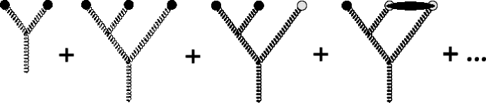
Figure 1: The diagrams contributing to the chromoelectric field at order $\alpha_{s}$. The full circles denote the background charge density $\rho$. The empty circles denote the average of the charge density induced by the fluctuations $<\delta\rho>=\sigma$. The black bars denote contractions corresponding to the mean fluctuation of the induced charge density $<\delta\rho\delta\rho>=\chi$.

It is clear that $\sigma^{a}_{i}$ is nothing but the average value of the induced chromoelectric field. Additionally, since the induced charge density $\delta\rho$ contains components with frequencies $p^{-}$ higher than those of the input charge density $\rho$, upon time averaging the induced chromoelectric field is characterized also by mean fluctuation $<\delta\alpha^{a}_{i}\delta\alpha^{b}_{j}>=\chi^{ab}_{ij}$. This again has the simple diagrammatic representation shown in Fig 2.

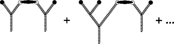
Figure 2: The average fluctuation of the induced chromoelectric field $\chi^{ab}_{ij}$. The notations are the same as in Fig.1.

The explicit expressions Eqs. (2), (14 and (16) are equivalent to resumming all the diagrams of the type indicated in Fig. 1 and Fig. 2. They clearly exhibit the mechanism of the evolution of the field correlators in our approach.

3 The Doubly Logarithmic Regime

We would now like to consider the evolution in the doubly logarithmic approximation. By this we mean that in every step of the evolution not only the longitudinal momenta are lowered but in addition, the transverse momenta are required to grow. That is of course just the QCD parton model picture that the ”valence” partons have transverse momenta on the typical hadronic scale while the high transverse momentum partonic components of a hadron exist only as fluctuations at short time scales. As discussed in [1] increasing the frequency in the evolution is equivalent to transverse momentum ordering in addition to the longitudinal momentum ordering. This scheme is therefore equivalent to the Born–Oppenheimer approximation in a system with a continuum of time scales.

Technically, in our approach the doubly logarithmic regime is singled out by restricting the transverse momenta in the fluctuation field which is being integrated over to be smaller than the transverse momentum of the observable that is being calculated, but larger than the transverse momentum of the background field. Practically this just means that the background field throughout the calculation is considered to be independent of $x_{\perp}$. The results are then easily obtained by taking the leading order of the transverse derivative expansion of the general expressions for $\chi$ and $\sigma$ given in [1]. The result in this limit simplifies very much for two main reasons. First, since there is ordering in all momentum components in the evolution it is clear that virtual diagrams can not give a non-vanishing contribution. This is simply the result of momentum conservation in the $x_{\perp}$ independent background. Therefore we have immediately

$$\sigma^{a}=\sigma^{a}_{i}=0\,.$$ (17)

The calculation of the real part also simplifies. This is because the two components of the chromoelectric field commute in this limit

$$[\alpha_{i},\alpha_{j}]=0$$ (18)

This is the consequence of the first equation in Eq. (4) for constant $\alpha_{i}$. This means that $\alpha_{i}$ can be treated as constant numbers. Using the explicit expressions from [1] for $\chi$ we obtain in the double logarithmic limit

$$\chi^{ab}(x,y)=-4\left[\alpha^{2}<x|\frac{(\partial D)^{2}}{D^{2}(\partial^{2}+2\alpha^{2})}|y>\right]^{ab}$$ (19)

and

$$\chi^{ab}_{ij}(x,y)=4\left[\alpha^{2}<x|\frac{D_{i}D_{j}}{D^{2}(\partial^{2}+2\alpha^{2})}|y>\right]^{ab}\,.$$ (20)

Let us first check that our expressions in the limit of weak field do indeed reproduce the DGLAP evolution in the double logarithmic regime, as claimed. To this end let us consider the evolution of the two point function .

$$\frac{d}{d\zeta}<\alpha_{i}^{a}(x)\alpha_{j}^{b}(y)>=4\alpha_{s}\left[<x|\alpha^{2}\frac{D_{i}D_{j}}{D^{2}(\partial^{2}+2\alpha^{2})}|y>\right]^{ab}$$ (21)

At weak fields the $2\alpha^{2}$ term in the denominator of Eq. (21) should be dropped and the covariant derivatives become simple derivatives. Taking trace of the evolution equation over both, color and transverse indices we obtain

$$\frac{d}{d\zeta}<\alpha_{i}^{a}(x)\alpha_{i}^{a}(y)>=-4\alpha_{s}N_{c}<\alpha_{i}^{a}\alpha_{i}^{a}><x|\frac{1}{\partial^{2}}|y>$$ (22)

The gluon distribution is related to the field correlator in the following way [1]

$$xG(Q) = (2\pi)^{2}\int d^{2}b<F^{+i}(b,xp^{+},x^{+})F^{+i}(b,xp^{+},x^{+})>_{Q}$$ (23)

$$= \frac{1}{4\pi\alpha_{s}}\int d^{2}b\int_{0}^{Q^{2}}d^{2}k\int d^{2}xe^{ikx}<\alpha_{i}^{a}(b+x/2)\alpha_{i}^{a}(b-x/2)>$$

Here $F^{+i}(b,k^{+})=\int dx^{-}e^{ik^{+}x^{-}}F^{+i}(b,x^{-})$ and the subscript $Q$ means that the transverse coordinates in the chromoelectric fields operators are equal with accuracy $1/Q$. This also gives

$$\frac{\partial}{\partial\ln Q^{2}}[xG(Q)]=\frac{1}{4\alpha_{s}}Q^{2}\int d^{2}b\int d^{2}xe^{iQx}<\alpha_{i}^{a}(b+x/2)\alpha_{i}^{a}(b-x/2)>$$ (24)

The factor $\frac{1}{4\pi\alpha_{s}}$ appears in these expressions since the vector potential $\alpha_{i}$ differs in normalization from the chromoelectric field by a factor $1/g$, see Eq. (3). Taking the Fourier transform of Eq. (22) and integrating over the impact parameter $b_{i}$ we obtain

$$\frac{\partial^{2}}{\partial\zeta\partial\ln Q^{2}}[xG(Q)]=\frac{\alpha_{s}N_{c}}{\pi}xG(Q)$$ (25)

which is precisely the double logarithmic approximation to the DGLAP equation.

The following comment is due here. The right hand side of Eq. (22) contains the expression $<\alpha_{i}^{a}\alpha_{i}^{a}>$. In the leading order of the derivative expansion $\alpha_{i}$ does not depend on the transverse coordinate, and this expression of course is also constant. If one allows slow variation of the field (slow in the sense that the scale of the spatial variation should be much larger than $1/Q$) this obviously should be understood as $<\alpha_{i}^{a}(b)\alpha_{i}^{a}(b)>$ where the impact parameter $b=(x+y)/2$ is the center of mass coordinate. Of course since the spatial resolution is $1/Q$, the coordinate of the field is only defined to this accuracy. The more exact specification can be only given beyond the leading order of the derivative expansion and is therefore beyond the approximation we are discussing here. Another way of saying this is that the fields that contribute to the right hand side of the evolution equation themselves contain only transverse momentum components smaller than $Q$. We therefore have to understand $<\alpha_{i}^{a}\alpha_{i}^{a}>$ on the right hand side of Eq. (22) as

$$<\alpha_{i}^{a}(b)\alpha_{i}^{a}(b)>=\int_{0}^{Q^{2}}\frac{d^{2}k}{4\pi^{2}}\int d^{2}xe^{ikx}<\alpha^{a}_{i}(b-x/2)\alpha^{a}_{i}(b+x/2)>$$ (26)

This is precisely how $G(Q)$ arises in the right hand side of Eq. (25). In this approximation therefore the dependence on $Q$ and $b$ in Eq. (22) factorizes and the products of the fields are defined with the transverse cutoff $1/Q$. This is a general feature of the leading order of derivative expansion and is not specific in any sense to the weak field limit.

We note that expanding the right hand side of Eq. (21) to second order in the field intensity and taking trace over color and Lorentz indices we obtain the first nonlinear correction to the DGLAP equation

$$\frac{\partial^{2}}{\partial\zeta\partial\ln Q^{2}}xG(Q)=\frac{\alpha_{s}N_{c}}{\pi}xG(Q)-{2\over Q^{2}}\int d^{2}b{\rm tr}<(\alpha(b)^{2})^{2}>$$ (27)

This is precisely the contribution of the twist four operator to the evolution of gluon density as calculated by Mueller and Qiu [21]. It is probably worthwhile noting that Eq. (27) should be compared not with the nonlinear GLR equation, which is expressed in terms of the distribution function, but rather with Eq. (25) of [21] which contains the contribution of twist four operators to the evolution of the gluon distribution. It is straightforward to check that taking into account the normalization of the operator $G^{(2)}$ in [21] our Eq. (27) is indeed equivalent to Eq. (25) of [21]. The nonlinear GLR equation arises as an approximation to this equation if one assumes factorization of the four gluon operator into the square of the gluon distribution in a very particular manner. Assuming this factorization Eq. (27) would indeed lead to the GLR equation with the same coefficient as given in [21].

Equations for the higher correlators can be analyzed in a similar fashion in the weak field limit. They all reduce to homogeneous evolution equations and yield simple expressions for the anomalous dimensions of the higher twist operators. Our main interest here, however, is to explore the opposite situation, namely when the fields and partonic densities become large and this is what we will do in the rest of this paper.

The most prominent feature of equation (21) is the appearance of the factor $Q^{2}-2\alpha^{2}$ in the denominator. The field strength $-2\alpha^{2}$ therefore plays the role of a dynamically generated mass in the evolution at high density. This is not entirely unexpected, but it is gratifying to see the emergence of this dynamical mass in such a straightforward fashion in our approach. Clearly the effect of this mass is to slow down the evolution. In fact it is easy to see that when the density becomes large this “mass term” dominates the evolution and leads to unitarization.

Let us consider the evolution of the distribution function in the high density -strong field limit $-\alpha^{2}>Q^{2}$. Neglecting $Q^{2}$ relative to $\alpha^{2}$ in the denominator in Eq. (21) we obtain

$$\frac{\partial^{2}}{\partial\zeta\partial\ln Q^{2}}xG(Q)=\frac{N_{c}(N_{c}-1)}{2}Q^{2}S$$ (28)

Here $S$ is the area of the hadron within which the density is high. It appears due to the integration over the impact parameter. The origin of the color factor $N_{c}(N_{c}-1)$ is the following. If the matrix $\alpha^{2}$ had no zero eigenvalues, this factor would be just $N_{c}^{2}-1$ - the trace of the unit matrix in the adjoint representation. However the matrices $\alpha_{i}$ as defined in Eq. (15) necessarily have zero eigenvalues. The number of these zero eigenvalues is generically $N_{c}-1$. Since $[\alpha_{i},\alpha_{j}]=0$, the same applies to the matrix $\alpha^{2}$. The contribution to the trace therefore comes only from the subspace spanned by the eigenvectors which correspond to nonzero eigenvalues. The dimensionality of this subspace is $N_{c}^{2}-1-(N_{c}-1)=N_{c}(N_{c}-1)$.

Integrating Eq. (28) we obtain

$$xG(Q^{2})=\frac{N_{c}(N_{c}-1)}{2}Q^{2}S\ln(1/x)+G_{0}$$ (29)

This result is very interesting. First it shows a characteristic feature expected of unitarization - the growth with energy is only logarithmic rather than power like as in the case of a pomeron, or $\exp\sqrt{\log s}$ as in the case of the doubly logarithmic DGLAP evolution. On the other hand the gluon density does not completely saturate but keeps growing logarithmically even at high densities. Similar “partial saturation” was found in the analysis of [10]. and also in the solution of a nonlinear evolution equation in [12].

Identifying naively the gluon distribution with the total DIS cross section for a probe that couples directly to gluons one would get a logarithmic growth of the cross section on top of the factor of the geometric area of the hadron. This is perfectly compatible with the Froissart bound and in fact grows slower than the allowed square of the logarithm if the effective area $S$ in Eq. (29) grows slower than logarithmically. On the other hand the prefactor depends strongly on the number of colors and is large at large $N_{c}$. This is not what one expects generically from the unitarized cross section. Once the geometric size has been factored out one does not expect any other numerical factors. The factor $N_{c}^{2}$ is of a purely perturbative origin. It counts the number of perturbative degrees of freedom - gluons that take part in the scattering. This is in accord with the fact that our approach is indeed perturbative and we therefore can only detect the perturbative mechanism for unitarization which should be operative in the region where the scattering is mainly perturbative. Apart from the perturbative component which is described by our present approach there is also a nonperturbative, low transverse momentum one of the soft pomeron type (see e.g. the recent analysis in [22]) which is not governed by the evolution we consider here. At very low values of $x$ it must become leading and eventually the perturbative behavior of Eqs. (28), (29) will cross over into the real asymptotics which may behave as a square of the logarithm.

4 The Gaussian model.

Eq. (29) represents the asymptotics of the distribution at large values of the density. At small $x$ one expects the density to be large close to the center of a hadron, at small values of the impact parameter, but not near the boundary. Eq. (28) therefore can not be quite correct even at small $x$. To get a more realistic picture one has to allow for a possibility of a more rapid evolution in the peripheral regions.

Generically the system of equations Eq. (2) is a coupled system of equations for infinite number of the multi gluon correlation functions and as such is nontrivial even in the doubly logarithmic limit. We would like to simplify this system so that it becomes more tractable. One straightforward possibility is to consider a Gaussian truncation of the original system. What we mean by this is to assume standard Gaussian factorization of multi particle correlators of the type

$$<\alpha^{2n}>\sim(2n-1)!!<\alpha^{2}>^{n}$$ (30)

This approximation is in the spirit of the GLR model [9].

Technically this means that we take the statistical weight used for calculation of the averages on the right hand side of the evolution equation as a Gaussian function of the fields. One should of course take care to ensure that this Gaussian weight is consistent with the symmetries of the system and also with the fact that the two spatial components of the chromoelectric field are not completely independent but rather commute with each other, see Eq. (18). To ensure this, let us explicitly solve the constraint commutativity imposes on the matrices $\alpha_{i}$. The quantities to be averaged all being invariant under global color rotations implies they can only depend on the eigenvalues of the $\alpha_{i}$. Since the $\alpha_{i}$ commute, they can be diagonalized simultaneously. We can therefore take the following explicit representation

$$\alpha_{i}=i\sum_{A}t_{i}^{A}T^{A}$$ (31)

Here $T^{A}$ are the diagonal Cartan subalgebra generators of the SU(N) group in the adjoint representation, $t_{i}^{A}$ are real coefficients and the index $A$ takes values from 1 to $N_{c}-1$. The coefficients $t_{i}^{A}$ are completely independent and the Gaussian weight for the averaging can be taken as

$$<...>=\left(\frac{(N_{c}-1)}{\alpha_{s}xg}\right)^{N-1}\int\Pi_{i,A}dt_{i}^{A}\ ...\ \exp\left\{-\frac{\pi(N_{c}-1)}{\alpha_{s}xg}t_{i}^{A}t_{i}^{A}\right\}$$ (32)

The meaning of the parameter $g$ is made clear by calculating the glue–glue correlator

$$<\alpha_{i}^{a}\alpha_{i}^{a}>=\frac{\alpha_{s}}{\pi}xg\,.$$ (33)

The quantity $g$ is therefore the local partonic density. Just as the field itself it is of course a slowly varying function of the impact parameter, and is related to the gluon distribution by

$$G(x,Q^{2})=\int d^{2}b_{\perp}g(x,b_{\perp},Q^{2})$$ (34)

Fourier transforming Eq. (21) and taking trace we get for the right hand side

$$4\alpha_{s}\sum_{n=1}^{N_{c}^{2}-1}<\frac{t_{i}^{A}t_{i}^{B}r_{n}^{A}r_{n}^{B}}{Q^{2}+2t_{j}^{C}t_{j}^{D}r_{n}^{C}r_{n}^{D}}>$$ (35)

where $r_{n}^{A}$ is the $n$-th eigenvalue of the $A$-th Cartan subalgebra generator in the adjoint representation. The $N_{c}-1$ dimensional vectors ${\bf r}_{n}$ are the root vectors of $SU(N)$ and have the following important properties

$${\bf r}_{n}^{2} = 0,\ \ \ \ n=1,...,N_{c}-1$$ (36)

$${\bf r}_{n}^{2} = 1,\ \ \ \ n=N_{c},...,N_{c}^{2}-1$$

Therefore only the terms $n=N_{c},...,N_{c}^{2}-1$ contribute to the sum. In each one of these non vanishing terms one can perform an orthogonal rotation of the coefficients $t_{i}^{A}\rightarrow s_{i}^{A}$ such that

$$s_{i}^{1}=t_{i}^{A}r_{n}^{A}$$ (37)

The possibility of such an orthogonal rotation is assured by the fact that the root vectors are properly normalized. The expression in Eq. (35) then simplifies to

$$\frac{4N_{c}(N_{c}-1)^{2}}{xg}\int ds_{i}\exp\left\{-\frac{\pi(N_{c}-1)}{\alpha_{s}xg}\ s_{i}^{2}\right\}\frac{s_{i}^{2}}{Q^{2}+2s_{i}^{2}}$$

$$= \frac{\pi N_{c}(N_{c}-1)^{2}Q^{2}}{xg}\int_{0}^{\infty}ds\left[\frac{s}{1+s}\right]\exp\left\{-\frac{\pi(N_{c}-1)Q^{2}}{2\alpha_{s}xg}\ s\right\}$$

The evolution equation then becomes

$$\frac{\partial^{2}}{\partial\zeta\partial\ln Q^{2}}xg(x,Q,b_{\perp})$$

$$= \frac{N_{c}(N_{c}-1)}{2}\ Q^{2}\bigg{[}1+\frac{\pi(N_{c}-1)Q^{2}}{2\alpha_{s}xg}\exp\left\{\frac{\pi(N_{c}-1)Q^{2}}{2\alpha_{s}xg}\right\}{\rm Ei}\left(-\frac{\pi(N_{c}-1)Q^{2}}{2\alpha_{s}xg}\right)\bigg{]}$$

where ${\rm Ei}(x)$ is the integral exponential function defined as

$${\rm Ei}(x)=-\int_{-x}^{\infty}\!dt\ \frac{e^{-t}}{t},\ \ \ \ x<0$$ (40)

We stress that the factorization assumed in Eq. (32) is motivated only to the extent that it leads to a closed evolution equation for the gluon density. One can think of it as a mean field approximation for the true weight function for the averaging over fields $\alpha_{i}$. One certainly expects this approximation to be valid at small $xg$ where it is equivalent to the steepest descent integration over $\alpha_{i}$’s. Additionally at large $xg$ the asymptotics of Eq. (4) reduces to the exact asymptotics of the original equation (21) and is independent of the form of the weight function. It is therefore reasonable to expect that this simple model provides a sensible interpolation of the evolution between the weak and strong density regimes.

Note that Eq. (4) governs the evolution of the gluon density $xg(b)$ and is local in the impact parameter space. It therefore contains more information on the structure of the hadron state than just the gluon distribution $xG(x,Q^{2})$. To determine the evolution of the gluon distribution $xG(x,Q^{2})$ one has to integrate the solution of Eq. (4) over the impact parameter $b$. To write down a closed equation directly for $xG$ one would have once again to resort to modeling. This time one needs a model of the gluon density as a function of the impact parameter. Models of this kind have indeed been used in the literature. One usually assumes a simple factorizeable structure [12] $g(x,Q^{2},b)=G(x,Q^{2})S^{-1}(b)$. The resulting equation for $G$ then depends on the form of $S(b)$ one takes in this ansatz. For example for a simple homogeneous disk model $S^{-1}(b)=(\pi R^{2})^{-1}\theta(R^{2}-b^{2})$, Eq. (4) with the substitution $Q^{2}\rightarrow Q^{2}\pi R^{2}$ governs the evolution of $xG$. More commonly one uses the Gaussian type distribution $S^{-1}(b)=(\pi R^{2})^{-1}e^{-{b^{2}\over 2R^{2}}}$. Any specific ansatz of this type introduces a new phenomenological parameter $R$ into the equation which has the meaning of an effective radius of the gluon distribution in the hadron. The same kind of parameter appears in the GLR equation [9, 21].

It would be interesting to study equation (4) numerically to find out how the effective area in which the partonic density is high ($S$ in Eqs. (28), (29)) depends on the rapidity. This we intend to do in a future publication.

5 Discussion

We have considered the doubly logarithmic limit of the low $x$ nonlinear evolution equations derived in [1]. The most salient feature in this regime is the appearance of a dynamically induced mass which leads to the slowdown of the evolution as the partonic density becomes larger. In particular we have shown that at small impact parameters the gluon density grows as a logarithm of energy rather than following the much faster growth pattern predicted by DGLAP evolution. To study the crossover between these two regimes in detail one has to analyze the set of equations (2) for the evolution of multi gluon correlators. This is still a formidable problem, although in the doubly logarithmic limit the equations are much simpler than the general evolution equations of [1].

We have discussed an approximation in which a closed equation Eq. (4) for the gluon density arises. This approximation imposes Gaussian factorization of multi particle operators in terms of the gluon density and is similar in spirit to the approximation used to write down the GLR equation in [9] and [21].

We note that the local equation for the gluon density Eq. (4) is qualitatively similar to the equation suggested in [12]. The authors of [12] suggested the following equation on the basis of reinterpretation of the Glauber formula for multiple scattering of [10]

$${\partial^{2}\over\partial\zeta\partial\ln Q^{2}}xg={2Q^{2}\over\pi^{3}}\left\{1-e^{-{N_{c}\alpha_{s}\pi^{2}\over 2Q^{2}}xg}\right\}$$ (41)

Although the functional form of this equation looks somewhat different from our Eq. (4) the main features are the same. Both reduce to the DGLAP equation in the limit of small density. Asymptotically at low $x$, where the density is high the solution to both equations behaves as $Q^{2}{\rm ln}1/x$.

There are however also important differences between the two equations. At large densities the correction to the asymptotic solution of Eq. (41) is exponentially small. On the other hand expanding Eq. (4) to order $1/xg$ we find

$$\frac{\partial^{2}}{\partial\zeta\partial\ln Q^{2}}xg(x,Q,b)=\frac{N_{c}(N_{c}-1)}{2}\ Q^{2}\left[1-\frac{\pi(N_{c}-1)Q^{2}}{2\alpha_{s}xg}\ln{2\alpha_{s}xg\over\pi(N_{c}-1)Q^{2}}\right]$$ (42)

So the correction here is a power enhanced by a logarithmic factor. The approach to the asymptotics is therefore much slower than in Eq. (41). Since the correction term is negative it is clear that the solution to Eq. (4) has a slower growth at low $x$. That is to say, at low densities solutions of both Eq. (41) and Eq. (4) start growing according to the double logarithmic DGLAP equation $xg\propto e^{\sqrt{\bar{\alpha}_{s}\ln 1/x}}$ (neglecting the running of $\alpha_{s}$). This growth however is tempered faster in the solution of Eq. (4) than in Eq. (41). One could wonder perhaps whether the existence of power corrections at large density in Eq. (4) is an artifact of the Gaussian truncation of the infinite set of equations Eq. (2). It is easy to see that this is not the case. The reason is that the mechanism of screening in our approach is the appearance of the effective mass proportional to the intensity of the chromoelectric field in Eq. (20). This type of screening with necessity gives power like preasymptotic corrections. It would be very interesting to understand better the relation between our present approach and the approach of [12].

Finally we note that in a recent very interesting paper [23] Makhlin and Surdutovich also considered the appearance of effective mass in the context of nuclear collisions. Their approach physically is complementary to ours. They consider the emission in the final state in a nuclear collision. In this situation the large transverse momentum modes are emitted first whereas the low transverse momenta are then emitted and propagate not in the vacuum but in the background of these hard modes. The propagation of soft modes in the preexisting hard mode background is then characterized by an effective mass. We on the other hand consider fast, large transverse momentum fluctuations in the hadron which develop on the background of a slower, smaller transverse momentum fields. At large fields the fluctuations are inhibited and this is the origin of the effective mass in our approach. It characterizes the emission of hard fluctuations in the preexisting soft field background.

Acknowledgements

We thank G. Levin, A. Makhlin and G. Surdutovich for interesting discussions.J.J-M was supported by the Director, Office of Energy Research, Office of High Energy and Nuclear Physics Division of the Deparment of Energy, under contract No. DE-AC03-76SF00098 and DE-FG02-87ER40328. A.K. is grateful to the Nuclear Theory group at LBL and the Theoretical Physics Institute, University of Minnesota for hospitality during April 1998 when part of this work was done. A.K. is supported by PPARC Advanced Fellowship. A.L. is partially supported by Russian Fund for Basic Research under Grant 96-02-16210. H.W. was supported by the EC TMR Program, contract ERB FMRX-CT96-0008. He is grateful to the Theoretical Physics Institute, University of Minnesota for their hospitality during March and April 1998 and wants to thank the Alexander von Humboldt Foundation for support during that stay.

References

- [1] J. Jalilian-Marian, A. Kovner and H. Weigert, hep-ph/9709432.
- [2] see e.g. Yu. Dokshitzer, V. Khose, A. Mueller and S. Troyan, ”Basics of Perturbative QCD”, ed. Frontiers, 1991.
- [3] E. Gotsman, E.M. Levin and U. Maor; hep-ph/9708275.
- [4] H. Abramowicz, L. Frankfurt and M. Strickman, hep-ph/9503437.
- [5] A. Mueller, hep-ph/9710531, Eur. Phys.J. A1 (1998) 19.
- [6] E. Gotsman, E.M. Levin and U. Maor; hep-ph/9606280 Nucl. Phys. B493 (1997) 354.
- [7] A. Hebecker and H. Weigert; hep-ph/9804217.
- [8] E. Levin, Talk at ”Continuous Advances in QCD”, Minneapolis, April 1998, hep-ph/9806434; see also E. Levin, hep-ph/9709226 and E. Gotsman, E. Levin and U. Maor, hep-ph/9712517.
- [9] L.V. Gribov, E.M. Levin and M.G. Ryskin, Phys. Rep 100 (1981).
- [10] A.H. Mueller, Nucl. Phys.B335 (1990), 115.
- [11] E. Laenen and E. Levin, Nucl. Phys. B451 (1995), 297.
- [12] A. L. Ayala, M. B. Gay Ducati and E. M. Levin hep-ph/9706448 Nucl.Phys. B511 (1998) 355.
- [13] J. Jalilian - Marian, A. Kovner, L. Mc Lerran and H. Weigert Phys.Rev. D55 (1997) 5414, hep-ph/9606377;
- [14] J. Jalilian-Marian, A. Kovner, A. Leonidov and H. Weigert, hep-ph/9701284 Nucl. Phys.B504 (1997) 415.
- [15] J. Jalilian-Marian, A. Kovner, A. Leonidov and H. Weigert, hep-ph/9706377.
- [16] L.N. Lipatov, Nucl. Phys. B452 (1995), 369; Phys. Repts. 286 (1997), 131.
- [17] V.T Kim and G.B. Pivovarov, Phys. Rev. Lett. 79 (1997), 809.
- [18] I. Balitsky, Nucl. Phys. B463 (1996), 99; hep-ph/9706411.
- [19] L. McLerran and R. Venugopalan, Phys. Rev. D49 (1994) 2233, hep-ph/9309289, Phys. Rev. D49 (1994) 335, hep-ph/9311205; A. Ayala, J. Jalilian-Marian, L. McLerran and R. Venugopalan, Phys.Rev. D53 (1996) 458, hep-ph/9508306;
- [20] In preparation.
- [21] A.H. Mueller and J.W. Qiu, Nucl. Phys. B268 (1986), 427.
- [22] A. Donnachie and P.V. Landshoff, hep-ph/9806344.
- [23] A. Makhlin and E. Surdutovich, hep-ph/9803364.