Solar Antineutrinos from Fluctuating Magnetic Fields at Kamiokande.

Abstract

We consider the effect of a strongly chaotic magnetic field at the narrow bottom of the convective zone of the Sun together with resonant matter oscillations on the production of electron Majorana antineutrinos. Even for moderate levels of noise, we show that it is possible to obtain a small but significant probability for $\nu_{e}\to\overline{\nu}_{e}$ conversions (1-3%) at the energy range 2-10 MeV for large regions of the mixing parameter space while still satisfying present (Super)-Kamiokande antineutrino bounds and observed total rates. In the other hand it would be possible to obtain information about the solar magnetic internal field if antineutrino bounds reach the $1\%$ level and a particle physics solution to the SNP is assumed. The mechanism presented here has the advantage of being independent of the largely unknown magnetic profile of the Sun and the intrinsic neutrino magnetic moment.

PACS: 14.60.Pq; 13.10.+q; 13.15.+g; 02.50.Ey; 05.40.+j; 95.30.Cq; 98.80.Cq.

Key words: neutrino, magnetic moment, magnetic fields, random equations.

1. The combined action of spin flavour precession in a magnetic field and ordinary neutrino matter oscillations can produce an observable flux of $\overline{\nu}_{eR}$’s from the Sun in the case of the neutrino being a Majorana particle.

Water Cerenkov detectors such as Kamiokande and SuperKamiokande (SK) which are sensitive to the $\nu_{e}-e$ elastic interaction are also capable of detecting these $\overline{\nu}_{e}$’s coming from the sun. Forthcoming solar neutrino experiments, such as SNO and Borexino are also expected to have a high sensitivity to them.

The specific signature of electron antineutrinos in proton containing materials is the inverse beta decay process: $\overline{\nu}_{e}+p\to n+e^{+}$, which produces almost isotropical monoenergetic positrons with a relatively high cross section. Antineutrino events would contribute in this way to the isotropic background.

Kamiokande data yielded restrictive limits on solar $\overline{\nu}_{eR}$ in the high energy region: for $E_{\nu}>9.3$ MeV the antineutrino total flux does not exceed $6-10\%$ of the SM predictions for the $\nu_{e}$ flux in the same energy range [1, 2]. Fiorentini et Al. [3] have shown that a better sensitivity can be achieved by exploiting the huge statistics of SK in conjunction with the residual directionality of the positrons from inverse beta decay. They pointed out that the angular dependence of the cross section can be used as a ”signature” for the presence of positrons from antineutrinos. Using their method not only upper bounds can be obtained but antineutrinos can actually be detected. From SK data corresponding to the first 101.9 days of observation they obtain a model independent bound $\Phi_{\overline{\nu}}(E_{\overline{\nu}}>8.3$ MeV$)<9.10^{4}$ cm^-2 s^-1 (C.L. 95%). This bound corresponds approximately to a fraction $\approx 5.2\%$ of the solar neutrino flux in the energy range considered predicted by the SSM. It is claimed that in a 3 year period of data taking SK could be sensitive to $\nu_{e}-\overline{\nu}_{e}$ oscillations at the $1-3\%$ level.

Bounds on the fraction of $\overline{\nu_{e}}$ can be translated into constraints on the neutrino mixing parameters if a specific model is assumed. Alternatively, solar properties associated with specific astrophysical models (i.e. convective solar magnetic fields) can be restricted by the absence of observance of antineutrinos. In the positive side, if we search for antineutrino appearance, the main question is to identify possible mechanisms which, over large regions of parameter space (i.e. without excessive fine-tuning) produce simultaneously relatively small quantities of $\overline{\nu_{e}}$ at Kamiokande energies in order to satisfy present experimental bounds but still produce significant quantities detectable at other experiments. It is not neccesary that the same mechanism be the responsible for all, the explanation of the absolute solar deficit, possible time variations of the signal and the production of antineutrinos. It is important then in this respect that the region of the parameter space where every effect is important be as large as possible.

Different concrete scenarios involving magnetic fields have been proposed where antineutrino generation is sizeable [1, 3]. The main problems of ”hybrid” models where a spin-flavour magnetic moment transition gives $\mbox{$\nu_{eL}$}\to\mbox{$\overline{\nu}_{\mu R}$}$ and mass-matter oscillations yields $\mbox{$\overline{\nu}_{\mu R}$}\to\mbox{$\overline{\nu}_{eR}$}$ transitions are to our opinion: a) The, nearly complete, lack of knowledge of the magnetic properties in the interior of the Sun. b) The high values, orders of magnitude higher than predicted by SM, of the magnetic moment which are needed to obtain any kind of sizeable effect. c) The undesirable large time variations of the neutrino flux which are usually associated with them.

In this work we present a new mechanism for antineutrino production inside the Sun which is largely model independent. We will consider the influence of a thin wall of highly chaotic magnetic field on the propagation of neutrinos in matter. For simplicity and in order to clearly expose the specific properties of the model we will disregard the influence of any other regular magnetic field. A similar model, which includes an additional constant field but disregards neutrino flavour mixing has been studied in [4]. As it has been noted in [4], some advantages of neutrino propagation in random magnetic fields include: a) The no neccesity to know in detail specific magnetic profiles. b) The potentially stronger effect of the random magnetic field in comparison to regular magnetic field: for the latter the spin precession is roughly proportional to the quantity $\exp C\int drB(r)$ where the integral is extended over the region where the magnetic field $B$ is present. However for the case of random magnetic fields the precession is proportional to $\exp C^{\prime}\int drB^{2}(r)$. In addition the chaotic precession is irreversible and regeneration effects of the original neutrino flux are absent or reduced. c) It is still important to assume a large transition magnetic moment $\mu$ for the neutrino, but the dependence on it is substantially altered. While for regular oscillations the constant $C\sim\mu$, for random magnetic fields $C^{\prime}\sim\Omega^{2}L_{0}\mu^{2}$. The dependence on the magnetic moment $\mu$ can be traded off, at least partially, for the dependence on the parameters $\Omega^{2},L_{0}$. These parameters describe the randomness and the coherence length of the magnetic field, they can be potentially very large, with an accepted range of variation of $\sim 1-3$ orders of magnitude. d) The overall influence of the random nature of the magnetic field is the flattening of the neutrino spectrum. The strong energy dependence on resonances is reduced, so this scenario is a natural way to avoid strong time variations.

The plan for the rest of this work is as follows. In the next paragraphs we will justify qualitatively the presence of chaotic magnetic fields in the convective region of the sun; next we will summarize the formalism of the neutrino propagation in random media; finally we will present the results. We will compute the antineutrino yield and total neutrino rate in Superkamiokande for different energy thresholds and compare with existing bounds. The SNO antineutrino production should follow a similar trend as that one calculated here of SK.

3. Very little is known, both theoretically and observationally, about the structure of the magnetic field inside the Sun [5, 6, 7, 8]. The absence of a significant external poloidal field precludes the existence of an internal core field or at least strongly limits its magnitude. The evidence of surface magnetic activity and the solar cycle indicate however the existence of a certain degree of magnetic activity in the upper layer, the convective zone. The existence of surface magnetic fields spatially localized (the typical size of a sunspot is $\sim 1000$ km) which fluctuate rapidly on time has been shown to exist ([9], as cited in Ref.[10]). It has been deduced that a similar picture should hold in the convective zone. On the other hand, the migration of the toroidal field towards the equator, the 11-year oscillation in sunspot number and the Hale-Nicholson law, can all be understood if it is assumed that a dynamo mechanism is effective in the convective region of the Sun. Direct numerical simulations of the magnetohydrodinamic turbulence show that for a large magnetic Reynolds number the magnetic field becomes indeed spatially intermittent [8].

It is generally accepted or at least strongly favored that a highly chaotic field, fluctuations of large amplitude and short length scale ($L_{0}\approx 10^{1}-10^{4}$ Km), could be effective in the convective zone specially in the hydrodinamically unstable region separating it from the core. From solar neutrino evidence: Kamiokande has shown repeteadly that there is not any significant semiannual variation of the neutrino flux. As it was pointed out in [10, 2], if a magnetic interaction of $\nu_{e}$’s in the sun takes place, the Kamiokande result ”implies” the dominance of the stochastic magnetic field over the large scale magnetic field.

In this work we will adopt the simplest option, we will ignore any large scale magnetic fields and assume the existence of a thin region where a purely chaotic field is present. Outside this layer a neutrino created at the solar interior experiences standard matter oscillations and the MSW effect. While traversing the chaotic region, the master Equation governing the time evolution of the 4x4 (2 flavors are assumed by simplicity) density matrix $\rho(t)$ is of the form:

$$i\partial_{t}\rho = [H_{0},\rho]+\mu\tilde{B}_{x}(t)[V_{x},\rho]+\mu\tilde{B}_{y}(t)[V_{y},\rho].$$ (1)

The $\tilde{B}_{x},\tilde{B}_{y}$ are the Cartesian transversal components of the chaotic magnetic field. Vacuum mixing terms and matter terms corresponding to the SSM density profile are all included in $H_{0}$. The matrices $V_{x,y}$ are given in terms of the Pauli matrices $\sigma_{1,2}$ by:

$$V_{x}=\pmatrix{0&i\sigma_{2}\cr-i\sigma_{2}&0},\quad V_{y}=\pmatrix{0&-i\sigma_{1}\cr i\sigma_{1}&0}.$$ (2)

We assume that the components $\tilde{B}_{x},\tilde{B}_{y}$ are statistically independent, each of them characterized by a $\delta$-correlation function:

$$\langle\tilde{B}_{x,y}(t)\tilde{B}_{x,y}(t^{\prime})\rangle = \langle\tilde{B}_{x,y}^{2}\rangle L_{0}\delta(t-t^{{}^{\prime}}),\quad\langle\tilde{B}_{x}(t)\tilde{B}_{y}(t^{\prime})\rangle=0.$$ (3)

We will assume equipartition among components: $\langle\tilde{B}_{x}^{2}\rangle=\langle\tilde{B}_{y}^{2}\rangle=\langle\tilde{B}^{2}\rangle/3.$ The length scale $L_{0}$ is a basically unknown parameter. It has been shown numerically and justified qualitatively in [11] that the $\delta$-correlation function is a sufficiently good approximation to more realistic finite correlators even for relative large correlation lengths.

The averaged evolution equation is a simple generalization (see Ref. [11] for a complete derivation) of the well known Redfield equation for two independent sources of noise [12] and reads ($\Omega^{2}\equiv L_{0}\mu^{2}\langle\tilde{B}^{2}\rangle/3$):

$$i\partial_{t}\mbox{$\langle\rho\rangle$}=[H_{0},\mbox{$\langle\rho\rangle$}]-i\Omega^{2}[V_{x},[V_{x},\mbox{$\langle\rho\rangle$}]]-i\Omega^{2}[V_{y},[V_{y},\mbox{$\langle\rho\rangle$}]].$$ (4)

It is possible to write the Eq.(4) in a more evolved form. Taking into account the particular form of the matrices $V_{x,y}$ and rescaling the density matrix according to:

$$\mbox{$\langle\rho(t)\rangle$}=\exp(-4\Omega^{2}t)\mbox{$\langle\rho^{\prime}(t)\rangle$},$$

the double commutators simplify and the evolution equation finally reads:

$$i\partial_{t}\mbox{$\langle\rho^{\prime}\rangle$}=[H_{0},\mbox{$\langle\rho^{\prime}\rangle$}]+i2\Omega^{2}\left(V_{x}\mbox{$\langle\rho^{\prime}\rangle$}V_{x}+V_{y}\mbox{$\langle\rho^{\prime}\rangle$}V_{y}\right).$$ (5)

It is useful however to consider the solution to Eq.(5) when $H_{0}\equiv 0$. This is the appropriate limit when dealing with extremely low $\Delta m^{2}$ or very large energies, for an extreme level of noise or when the distance over which the noise is acting is small enough to consider the evolution driven by $H_{0}$ negligible. In any other scenario it can give at least an idea of the general behavior of the solutions to the full Eq.(5). When $H_{0}=0$ only the two last terms in the equation remain and an exact simple expression is obtainable by ordinary algebraic methods. The full 4x4 Hamiltonian decouples in 2x2 blocks. The quantities of interest, the averaged transition probabilities, are given by the diagonal elements of $\langle\rho\rangle$. If $P_{f,i}$ are the final and initial probabilities ( at the exit and at the entrance of the noise region) their averaged counterparts fulfill linear relations among them, schematically:

$$Q_{f}^{A,B} = MQ_{i}^{A,B}$$ (6)

with $Q^{A,B}$ any of the two dimensional vectors

$$Q^{A}=\pmatrix{\langle P(\nu_{eL}\to\nu_{eL})\rangle\cr\langle P(\nu_{eL}\to\tilde{\nu}_{\mu R})\rangle};\quad Q^{B}=\pmatrix{\langle P(\nu_{eL}\to\tilde{\nu}_{eR})\rangle\cr\langle P(\nu_{eL}\to\nu_{\mu L})\rangle}\quad$$ (7)

and the Markovian matrix $M$ (with $P=1/2\left(1+\exp(-4\Omega^{2}\Delta t)\right)$):

$$M = \pmatrix{P&1-P\cr 1-P&P}.$$ (8)

The quantity $P$ is a good approximation for the depolarization that the presence of noise induces in the averaged neutrino density matrix. $\Delta t$ is the distance over which the noise is acting.

From Eqs.(6-7) we have in particular the relation

$$\langle P(\nu_{eL}\to\tilde{\nu}_{eR})\rangle_{f}=(1-P)\langle P(\nu_{eL}\to\nu_{\mu L})\rangle_{i}$$ (9)

in the case of the initial number of electron antineutrinos at the entrance of the noise wall being zero. The final number is proportional to the initial number of muon neutrinos. This number might be large if $1-P$ is not small and if the neutrino have passed through a MSW resonance before arriving to the noise region. The MSW resonance converts practically all the initial $\overline{\nu}_{e}$ flux into $\overline{\nu}_{\mu}$. The fluctuating magnetic field converts them into $\overline{\nu}_{e}$. Part of the electron antineutrinos will be reconverted into $\overline{\nu}_{\mu}$ by mass oscillations (vacuum and non-resonant matter oscillations). This reconversion is limited in this case, in contrast with regular magnetic fields, by the irreversible character of Eq.(5)

4. The averaged master equation (5) has been integrated numerically for a variety of mixing parameters ($\Delta m^{2},\sin^{2}2\theta$) and randomness parameter $P$. The parameter $P$ has been varied between its maximum and minimum values (respectively 1, absence of magnetic field, 1/2, complete depolarization of the density matrix). The corresponding r.m.s fields are in the range $\surd{\langle\tilde{B}^{2}\rangle}=0-600$ kG (supposing the scale $L_{0}=1000$ Km and $\mu=10^{-11}\mu_{B}$).

We have defined the weighted electron antineutrino appearance probability:

$$\langle P_{\nu_{e}\overline{\nu}_{e}}\rangle = \frac{\int_{E>Eth}dE\ \sigma(E)\Phi(E)P_{\nu_{e},\overline{\nu}_{e}}(E)}{\int_{E>Eth}dE\ \sigma(E)\Phi(E)}$$ (10)

where $\sigma(E),\Phi(E)$ are respectively the differential cross section for the isotropic background process $\overline{\nu}_{e}+p\rightarrow e^{+}n$ and the differential total neutrino flux coming from the Sun according to the SSM [13]. A constant experimental detector efficiency has been assumed over all the energy range. Three different illustrative threshold energies have been chosen $E_{th}=8.3,5.5$ and $2.0$ MeV. For $E_{th}<7.0$ MeV, the weighted probability varies modestly because the product $\sigma\Phi$ is strongly peaked around $E\approx 9-10$ MeV.

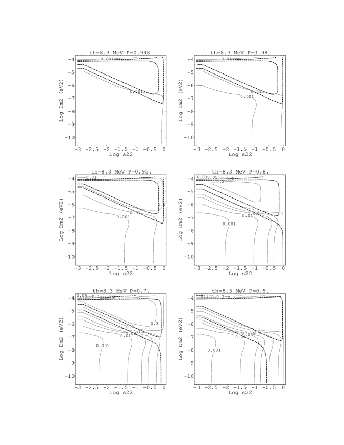
Figure 1: Continuous lines: $\overline{\nu_{e}}$ production as a function of neutrino mixing angle $\log\sin^{2}2\theta$ and $\Delta m^{2}$ (eV²). The average probability, Eq.(10), is given for different levels of noise. Dashed thick lines (not labeled): $S/S_{SSM}$ rates at SK, contours correspond to $S/S_{SSM}=0.3,0.5$ The threshold neutrino energy is in this case: $E_{th}=8.3$ MeV. From left to right and from top to bottom: $P=0.998,0.98,0.95,0.8,0.7,0.5$. The corresponding r.m.s fields are $\surd{\langle\tilde{B}^{2}\rangle}=15,45,65,150,220$ and 600 kG respectively (supposing the scale $L_{0}=1000$ Km and $\mu=10^{-11}\mu_{B}$).

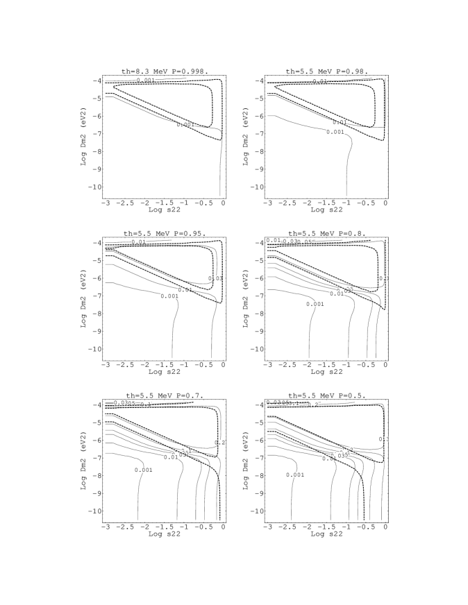
Figure 2: Idem as Fig.(1) for $E_{th}=5.5$ MeV. The dashed line corresponds to the existing experimental bound ($P<5\%$) from SK.

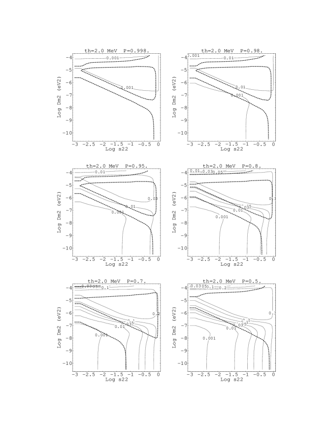
Figure 3: Idem as Figs.(1) and (2) for an energy threshold $E_{th}=2.0$ MeV.

In calculating the expected total signal rates, the elastic cross sections for the processes $\nu_{x}e\to\nu_{x}e$ with $\nu_{x}=\nu_{e},\nu_{\mu},\overline{\nu}_{e},\overline{\nu}_{\mu}$ has been taken from [14]. The results are shown in Figs.(1,2,3) corresponding respectively to each of the threshold energies which are considered. The continuous lines in the figures correspond to the contours for $\langle P_{\nu_{e}\overline{\nu}_{e}}\rangle$. The dashed thick lines correspond to the ratio of theoretical to SSM predicted total signal (S/S_SSM).

The characteristic MSW triangular contours are apparent in the figures, coinciding for both antineutrino and total rates. Note however how they shift independently as the threshold energy decreases. As the noise level increases, the 0.5 contour expands and the region compatible with present SK data enlarges. When combining total rates for the different solar neutrino experiments, the global allowed regions appear roughly at the three corners of the triangular regions (regions labeled as SMA, LMA and LOW MSW in, for example, Ref. [15]).

When the noise level is low ($P=0.95$ or higher), the bound $\langle P_{\nu_{e}\overline{\nu}_{e}}\rangle<\approx 0.05$ obtained [1, 3] from Kamiokande data is fulfilled for any point of the $(\Delta m^{2},\sin^{2}2\theta)$ parameter space considered. Nevertheless the antineutrino yield is non-negligible and is situated, in the range of values which could be experimentally tested in the near future [3]. For $P\approx 0.98$ there is a significant antineutrino production (1-3%) for practically all the region compatible with the total signal rate. This affirmation would continue to be true if the rest of solar neutrino experiments are taken into account (LMA and SMA regions). Only for the lowest $\Delta m^{2}$ compatible with SK total rate (the would-be LOW MSW region) we obtain an antineutrino probability smaller than 1%. Similar comments can be extracted from the plot corresponding to $P=0.95$. In this case the antineutrino yield increases to the $3-5\%$ level for the LMA and SMA regions and to $1-3\%$ for the LOW MSW region. The predictions for the $5.5$ and $2$ MeV thresholds are of similar character and no fundamental changes are observed: Similar levels of antineutrino production are expected in regions compatible with higher energy bounds.

Values for the noise parameter of $P=0.8$ or lower are not favored when we consider the combined total rates from the existing solar neutrino experiments at least in the limit of negligible mixing angle (see Ref.[4]). Let’s note that for these levels of noise, regions with a very high antineutrino yield are possible ($\langle P_{\nu_{e}\overline{\nu}_{e}}\rangle\approx 20-30\%$). Simultaneously, the region with a total rate compatible with SK results enlarges in the large angle limit. However the antineutrino production serves as a strong constraint: the consideration of the SK total rate and antineutrino production make that only marginal areas with $\Delta m^{2}\approx 10^{-8}$ eV² are still allowed. The same situation repeats at the $5.5$ MeV threshold. At $E_{th}=2$ MeV the predicted yield increases but is always in the $\sim<3\%$ level if we restrict ourselves to the areas allowed at higher thresholds.

5. In conclusion, in this work we have considered a model where solar neutrinos pass through a thin layer where chaotic magnetic field is present. Some comment is in order about the nature of the chaotic field considered here. According to [11] the $\delta$-correlation function is a sufficiently good approximation to more realistic finite correlators even for a relative large correlation length. Moreover, the quantity $P$ is connected with the depolarization of the density matrix, and therefore, it offers some advantage with respect to more ”physical” parameters as $\Omega^{2}$ or $\surd\langle\tilde{B}^{2}\rangle$: we expect that results expressed in terms of $P$ are largely independent of the concrete modelizing of the stochastic properties of the fluctuating field (in particular the form of the correlator).

From the numerical results presented above, it is deduced that a small but significant quantity of antineutrinos is expected to be detectable in SuperKamiokande and other water Cerenkov experiments (SNO) in parameter regions compatible with present experimental bounds (including neutrino magnetic moment bounds). If the neutrino is a Majorana particle, the scenario proposed in this work predicts a significant quantity of antineutrinos (1-3%) even for a modest level of noise ($P>0.95$) in regions compatible with existing experimental evidence. Lowering the detection energy threshold the quantity of antineutrinos tends to increase, but only very gently. In the other hand it would be possible to obtain information about the solar magnetic internal field if antineutrino bounds reach the $1\%$ level and a particle physics solution to the SNP is assumed. If a squared mass difference of the order $\mbox{$\Delta m^{2}$}\approx 10^{-5}$ is preferred, there are two favored alternatives, either the neutrino is not a Majorana particle or the level of solar convective magnetic noise is small ($P\approx 1$). This is so because otherwise we would have too many antineutrinos at high energy. Note however that even in the most restrictive case a significant quantity of antineutrinos ($\sim 1\%$) might be detectable at lower energies close to the $n$ production threshold.

Acknowledgments.

I acknowledge V.B. Semikoz for drawing my attention to the problem, for many and useful discussions about solar magnetic fields and for pointing out to me numerous references. This work has been supported by DGICYT under Grant PB95-1077 and by a DGICYT-MEC contract at Univ. de Valencia.

References

- [1] E.Kh. Akhmedov, A. lanza, S.T. Petcov. Phys. Lett., B 348 (1995) 124-132.
- [2] V.B. Semikoz. hep-ph/9611383 .
- [3] G. Fiorentini, M. Moretti, F.L. Villante. hep-ph/9801111 .
- [4] E. Torrente-Lujan. hepph/9807371.
- [5] E. N. Parker. Cosmical Magnetic Fields. Clarendon Press, Oxford, 1979.
- [6] E. N. Parker. Astrophys. J., 408 (1993) 707.
- [7] S.I. Vainstein, A.M. Bykov, I.M. Toptygin. Turbulence, Current Sheets and Shocks in Cosmic Plasma. Gordon and Breach, 1993.
- [8] S.I. Vainshtein, Y.B. Zeldovich and A.A. Ruzmakin, Turbulent dynamo in Astrophysics. Nauka, Moskow, 1980.
- [9] J. Stenflo, Astronom. Astrophys. Rev. 1 (1989) 3.
- [10] A. Nicolaidis. Phys. Lett., B 262 (1991) 303-306.
- [11] E. Torrente-Lujan. hepph/9807361.
- [12] F.N. Loreti, A.B. Balantekin. Phys. Rev. D50 (1994), pp. 4762–4770.
- [13] J.N. Bahcall and M.H. Pinsonneault, Rev. Mod. Phys. 67 (1995) 781.
- [14] S. Pastor, V.B. Semikoz, J.W.F. Valle. Phys. Lett. B369 (1996) 301-307.
- [15] J.N. Bahcall, P.I. Krastev and A.Y. Smirnov, hep-ph/9807216.