Preprint YERPHI-1520(20)-98
hep-ph/9807411

Infrared Quasi-Fixed Points and Mass Predictions in the MSSM

G. K. Yeghiyan

Yerevan Physics Institute,
Yerevan, Armenia

M.  Jurčišin and D. I. Kazakov

Bogoliubov Laboratory of Theoretical Physics, Joint Institute for Nuclear Research,
141 980 Dubna, Moscow Region, Russian Federation

1 Introduction

Supersymmetric extensions of the Standard Model are believed to be very promising theories to describe physics at energies to be reached by experiments in the near future. The most popular SM extension is the Minimal Supersymmetric Standard Model (MSSM) [1]. Although the MSSM is the simplest supersymmetric model, it contains a large number of free parameters. The parameter freedom of the MSSM comes mostly from soft supersymmetry breaking, which is needed to obtain a phenomenologically acceptable mass spectrum of particles. At the same time, a large number of free parameters decrease the predictive power of a theory. A common way to reduce this freedom is to make some assumptions at a high energy scale (for example, at the Grand unification (GUT) scale or at the Planck scale). Then, treating the MSSM parameters as running variables and using the renormalization group equations (RGE’s), one can derive their values at a low-energy scale.

The usual assumption is the so-called universality of soft-breaking terms at high energy. Within a supergravity induced SUSY breaking mechanism universality seems to be very natural and leads at low energies to a softly broken supersymmetric theory which depends on the following set of free parameters [1]: a common scalar mass $m_{0}$, a common gaugino mass $m_{1/2}$, a common trilinear scalar coupling $A$, a supersymmetric Higgs-mixing mass parameter $\mu$, and a bilinear Higgs coupling $B$. These parameters are defined at the high-energy scale and are treated as initial conditions for the RGE’s. The last two parameters can be eliminated in favour of the electroweak symmetry breaking scale, $v^{2}=v_{1}^{2}+v_{2}^{2}=(174.1\ GeV)^{2}$, and the Higgs fields vev’s ratio $\tan\beta=v_{2}/{v_{1}}$, when using minimization conditions of the Higgs potential. The sign of $\mu$ is unknown and is a free parameter of the theory.

Thus, using the concept of universality, one reduces the MSSM parameter space to a five dimensional one. It is also possible to restrict this remaining freedom. Namely, some low-energy MSSM parameters are insensitive to the initial values. This allows one to find their low-energy values without detailed knowledge of the physics at high energy. To do this one has to examine the infrared behaviour of RGE’s for these parameters and to find possible infrared fixed points.

Notice, however, that the true IR fixed points, discussed, e.g., in an earlier paper by Pendleton and Ross [2] are reached only in the asymptotic regime. For the ”running time” given by $\log M_{GUT}^{2}/M_{Z}^{2}$ they are reached only by a very narrow range of solutions. This problem has been resolved by consideration of more complicated fixed solutions like invariant lines, surfaces, etc. [3, 4, 5]. Such solutions turned to be strongly attractive: for the above-mentioned ”running time” the wide range of solutions of RGE’s ended their evolution on these fixed manifolds.

Here we are interested in another possibility connected with the so-called infrared quasi-fixed points first found out by Hill [6] and then widely studied by several authors [7]-[12]. These fixed points differ from Pendleton-Ross ones at the intermediate scale and usually give the upper (or lower) boundary for the relevant solutions.

Strictly speaking, these fixed points are not always relevant since the parameters of a theory do not necessarily have their maximum or minimum allowable values. For example, in the Standard Model the Hill fixed point for the top-quark Yukawa coupling corresponds to the pole top mass $m_{t}^{pole}=230$ GeV [5], which is excluded by modern experimental data [13].

The situation is quite different in the MSSM [9]-[12]: here the top-quark running mass is given by the equation

$$m_{t}=h_{t}v\sin{\beta}.$$ (1)

Now the Hill fixed point corresponds to physical values of the top mass when $\tan{\beta}$ is chosen appropriately.

It is remarkable that imposing the constraint of bottom-tau unification and radiative electroweak symmetry breaking leads to the value of the top Yukawa coupling close to its quasi-fixed point value [12, 14]. This serves as an additional argument in favour of the Hill-type quasi-fixed points. Therefore, in the present paper we assume $h_{t}(M_{Z})$ to be equal to its Hill fixed point value. We restrict ourselves to the consideration of low values of $\tan{\beta}$ for which one can neglect the bottom Yukawa coupling as compared to the top one.

A similar analysis has been performed in a number of papers [11, 15, 16, 17, 18, 19]. It has been pointed out that the IRQFP’s exist for the trilinear SUSY breaking parameter $A_{t}$ [15], for the squark masses [11, 16] and for the other soft supersymmetry breaking parameters in the Higgs and squark sector [19]. This allows one to reduce the number of unknown parameters and make predictions for the MSSM particle masses as functions of the common scalar and gaugino masses $m_{0}$ and $m_{1/2}$, respectively. In particular, in Ref.[17] the dependence of the lightest Higgs mass on the ratio $X=m_{0}/m_{1/2}$ has been studied.

In this paper, we perform a slightly different analysis. Based on the values of IRQFP’s for all soft terms and the known values of gauge couplings, top-quark and Z-boson masses, we determine the values of $\tan\beta$ and the $\mu$ parameter and then find masses of the Higgs bosons, stops and charginos. Our predictions are insensitive (or weakly sensitive) to the initial values of the ratios $m_{0}^{2}/m_{1/2}^{2}$ and $A_{0}/m_{1/2}$ in the wide range of variations. Due to this insensitivity the above-mentioned predictions depend only on one unknown parameter, the gluino mass. We find also the mass of the lightest Higgs boson as a function of the geometrical mean of stops masses, sometimes called the SUSY breaking scale. These results are confronted with the latest experimental data for searches of SUSY particles and of the Higgs boson.

The paper is organized as follows. In Section 2 we analyze RGE’s and IR quasi-fixed points. We use them in Section 3 to obtain the mass spectrum of the Higgs bosons and some SUSY particles. In Section 4 we discuss our main results and conclusions. Appendix contains some useful formulae.

2 Infrared Quasi-Fixed Points and RGE’s

In this section, we give a short description of the infrared quasi-fixed points (IRQFP) in the MSSM for the low $\tan\beta$ scenario. In this case, the only important Yukawa coupling is the top-quark one, $Y_{t}=h_{t}^{2}/(4\pi)^{2}$. It exhibits the IRQFP behaviour in the limit $Y_{0}=Y_{t}(0)\to\infty$  [6, 9, 10, 11, 15, 17]

$$Y(t)\Rightarrow Y_{FP}=\frac{E(t)}{6F(t)},$$ (2)

where $t=\log{M_{GUT}^{2}/Q^{2}}$ and the functions $E(t)$ and $F(t)$ are given in Appendix.

Though perturbation theory is not valid for $Y_{t}>1$, it does not prevent us from using the fixed point (2) since it attracts any solution with $Y_{0}\gg\tilde{\alpha}_{0}$ or, numerically, for $Y_{0}>0.1/4\pi$ (in fact, as one can see from Fig. 1a, this occurs for $Y_{0}>2\tilde{\alpha}_{0}$). Here $\tilde{\alpha}_{i}=\alpha_{i}/(4\pi)$ and $\tilde{\alpha}_{0}=\tilde{\alpha}_{i0}=\tilde{\alpha}_{i}(M_{GUT})$. Thus, for a wide range of initial values $Y_{t}$ is driven to the IR quasi-fixed point given by eq. (2) which numerically corresponds to $h_{t}(M_{Z})\approx 1.125$. It is useful to introduce the ratio $\rho_{t}\equiv Y_{t}/\tilde{\alpha}_{3}$. At the fixed point $\rho_{t}(M_{Z})\approx 0.84$. The low-energy value of $\rho_{t}$ is weakly dependent on its high-energy value $\rho_{0}$ when the latter is big enough. This allows one to use eq.(1) to predict the top-quark mass as a function of $\tan{\beta}$ [11]. Alternatively, one can use the IRQFP for $h_{t}$ to determine $\tan{\beta}$ for a given value of the running top-quark mass. We assume that the top Yukawa coupling has its Hill fixed point value $\rho_{t}(M_{Z})\approx 0.84$ and analyze the IRQFP behaviour of the SUSY breaking mass parameters in the MSSM with small $\tan{\beta}$. It is worth mentioning that our one-loop IRQFPs differ from those obtained in Ref. [19] due to ignorance of the electro-weak corrections to the IRQFPs in this paper. Contributions due to these corrections are more than 10% and have to be taken into account.

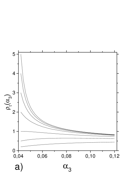
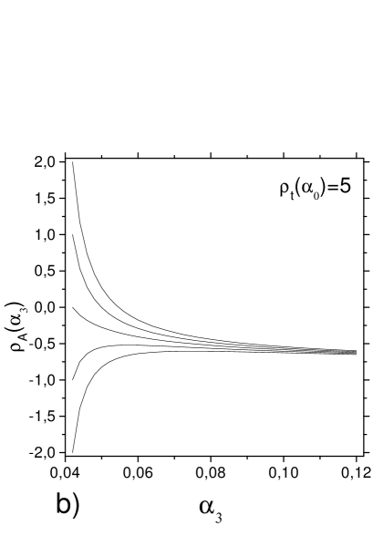
Figure 1: The infrared quasi-fixed points for $\rho_{t}=Y_{t}/\tilde{\alpha}_{3}$ (a) and $\rho_{A}=A_{t}/M_{3}$ (b)

As it has been noted already, we are interested in predictions for the Higgs bosons, the lightest chargino and the lightest squark (i.e. stop) masses. These masses depend on the Higgs mixing parameter $\mu$, the weak gaugino mass $M_{2}$, the soft masses from the Higgs potential $m_{H_{1}}^{2}$ and $m_{H_{2}}^{2}$, the squark masses $m_{Q}^{2}$ and $m_{U}^{2}$ (here Q refers to the third generation squarks doublet and U to the stop singlet), the trilinear stop soft coupling $A_{t}$ and $\tan{\beta}$. We determine $\tan{\beta}$ from eq.(1). The parameter $\mu$ is eliminated from the minimization condition of the Higgs potential. As for the remaining parameters, we express them via the common gaugino mass $m_{1/2}$ or, equivalently, via the gluino mass $M_{3}=(\tilde{\alpha}_{3}/\tilde{\alpha}_{0})m_{1/2}$, when analyzing their IR fixed point behaviour.

We perform the analysis of RGE’s at the one-loop level. The two-loop corrections have negligible impact on our results. We neglect also the effects connected with the mass thresholds and consider the supersymmetric RGE’s which are valid between the electroweak breaking scale $\sim M_{Z}$ and the GUT scale $\sim 10^{16}$ GeV. Our results are modified negligibly when the initial scale is chosen at $M_{Planck}\sim 10^{19}$ GeV.

The relevant RGE’s for soft supersymmetry breaking parameters are given in Refs. [20, 14]. The trilinear coupling $A_{t}$ in the limit $Y_{0}\to\infty$ possesses a IR quasi-fixed point (see Appendix for the notation)

$$\frac{A_{t}(t)^{FP}}{M_{3}}=-\frac{\tilde{\alpha}_{0}}{\tilde{\alpha}_{3}}\left(H_{2}-\frac{H_{3}}{F(t)}\right)\approx-0.62\,$$ (3)

independent of $A_{t}(0)=A_{0}$.

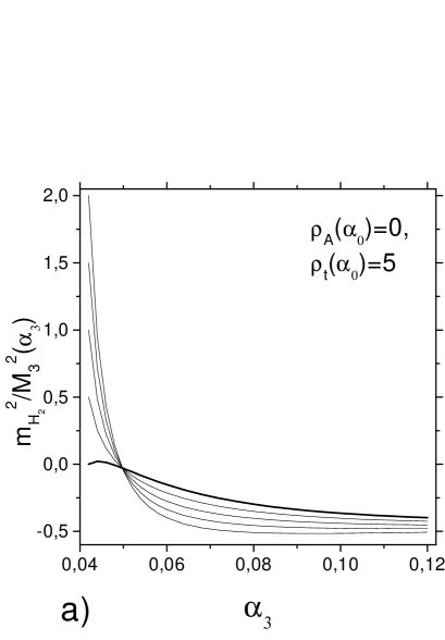
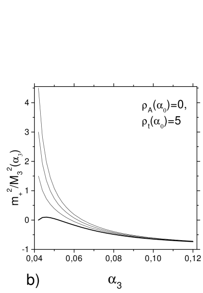
Figure 2: The infrared quasi-fixed points for $m_{H_{2}}^{2}/M_{3}^{2}$ (a) and $(m_{H_{1}}^{2}+2m_{H_{2}}^{2})/M_{3}^{2}$ (b)

The behaviour of $\rho_{A}=A_{t}/M_{3}$ as a function of $\tilde{\alpha}_{3}$ for a fixed ratio $Y_{0}/\tilde{\alpha}_{0}=5$ is shown in Fig. 1b. One can observe the strong attraction to the IR stable quasi-fixed point $\rho_{A}\approx-0.62$. In fact, all solutions corresponding to the small and moderate ratio $A_{0}/m_{1/2}$ ”forget” their initial conditions.

The RGE’s for $m_{H_{1}}^{2}$ and $m_{H_{2}}^{2}$ have the following solution  [20]:

$$m_{H_{1}}^{2} = m_{0}^{2}+m_{1/2}^{2}\tilde{\alpha}_{0}\left(\frac{3}{2}f_{2}(t)+\frac{3}{10}f_{1}(t)\right)\,,$$ (4)

$$m_{H_{2}}^{2} = m_{1/2}^{2}e(t)+A_{t}(0)m_{1/2}f(t)+m_{0}^{2}h(t)-k(t)A_{t}(0)^{2}\,,$$ (5)

where the functions $f_{i}(t)$, (i=1,2,3), $f(t)$, $h(t)$ and $k(t)$ are given in Appendix.

There is no obvious infrared attractive fixed point for $m_{H_{1}}^{2}$. However, one can take the linear combination $m_{+}^{2}=m_{H_{1}}^{2}+2m_{H_{2}}^{2}$ which together with $m_{H_{2}}^{2}$ shows the IR fixed point behavior in the limit $Y_{0}\to\infty$.

$$\frac{m_{+}^{2\ FP}}{M_{3}^{2}}=\left(\frac{m_{H_{1}}^{2}+2m_{H_{2}}^{2}}{M_{3}^{2}}\right)^{FP}=\frac{\tilde{\alpha}_{0}^{2}}{\tilde{\alpha}_{3}^{2}}\left(2\bar{e}(t)+\frac{3}{2}f_{2}(t)+\frac{3}{10}f_{1}(t)\right)\approx-0.73\,.$$ (6)

As for the ratio $m_{H_{2}}^{2}/M_{3}^{2}$, the solution for it has the following form:

$$\frac{m_{H_{2}}^{2\ FP}}{M_{3}^{2}}=\frac{\tilde{\alpha}_{0}^{2}}{\tilde{\alpha}_{3}^{2}}\left(\bar{e}(t)-\frac{1}{2}\frac{m_{0}^{2}}{m_{1/2}^{2}}\right)\approx-0.12\left(\frac{1}{2}\frac{m_{0}^{2}}{m_{1/2}^{2}}+3.4\right)\,.$$ (7)

In eq.(7) one has only weak dependence on the ratio $m_{0}^{2}/m_{1/2}^{2}$. This is because $\bar{e}(t)\sim\tilde{\alpha}_{3}^{2}/\tilde{\alpha}_{0}^{2}\gg 1$. One can find the IR quasi-fixed point $m_{H_{2}}^{2}/M_{3}^{2}\approx-0.40$ which corresponds to $m_{0}^{2}/m_{1/2}^{2}=0$. As for the combination $m_{+}^{2}$, the dependence on initial conditions disappears completely, as it follows from (6). The situation is illustrated in Fig.2.

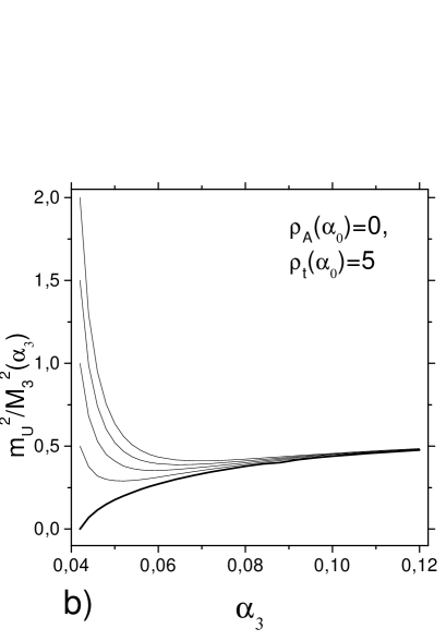
Figure 3: The infrared quasi-fixed points for $m_{Q}^{2}/M_{3}^{2}$ (a) and $m_{U}^{2}/M_{3}^{2}$ (b)

Now we consider the squark masses. The solutions to their RGE’s are given in Appendix. In the limit $Y_{t}\to\infty$ these solutions are driven to the IRQFP’s

$$\frac{m_{U}^{2\ FP}}{M_{3}^{2}} = \frac{\tilde{\alpha}_{0}^{2}}{\tilde{\alpha}_{3}^{2}}\left(\frac{2}{3}\bar{e}(t)+\frac{8}{3}f_{3}(t)-\frac{1}{2}f_{2}(t)+\frac{13}{30}f_{1}(t)\right)\approx 0.48$$ (8)

$$\frac{m_{Q}^{2\ FP}}{M_{3}^{2}} = \frac{\tilde{\alpha}_{0}^{2}}{\tilde{\alpha}_{3}^{2}}\left(\frac{1}{2}\frac{m_{0}^{2}}{m_{1/2}^{2}}+\frac{1}{3}\bar{e}(t)+\frac{8}{3}f_{3}(t)+f2(t)-\frac{1}{15}f_{1}(t)\right)$$ (9)

$$\approx 0.12\left(\frac{1}{2}\frac{m_{0}^{2}}{m_{1/2}^{2}}+5.8\right)$$

As it follows from eq.(8), the solution for $m_{U}^{2}/M_{3}^{2}$ becomes independent of the initial conditions $m_{0}/m_{1/2}$ and $A_{0}/m_{1/2}$, when the top-quark Yukawa coupling is initially large enough. As a result, the solutions of RGE’s are driven to the fixed point $m_{U}^{2}/M_{3}^{2}\approx 0.48$ for a wide range of $m_{0}^{2}/m_{1/2}^{2}$ (Fig.3b). As for $m_{Q}^{2}$, the dependence on initial conditions does not completely disappear; however, it is rather weak like in the case of $m_{H_{2}}^{2}$ and approaches the value $m_{Q}^{2}/M_{3}^{2}\approx 0.69$ (Fig.3a).

Thus, one has two kinds of infrared quasi-fixed points. For the first one ($m_{+}^{2}/M_{3}^{2}$ and $m_{U}^{2}/M_{3}^{2}$) the dependence on initial values disappears completely when the limit $Y_{0}\to\infty$ is considered. As a result, these fixed points attract any solution corresponding to small and moderate values of the ratio $m_{0}^{2}/m_{1/2}^{2}$ (Fig. 2b, Fig. 3b). For the second kind of IRQFP’s ($m_{H_{2}}^{2}/M_{3}^{2}$ and $m_{Q}^{2}/M_{3}^{2}$) weak dependence on initial values persists; these fixed points exist due to the fact that $\tilde{\alpha}_{3}^{2}/\tilde{\alpha}_{0}^{2}\gg 1$. As a result, one has small deviations of the RGEs solutions from these fixed points when moderate values of the ratio $m_{0}^{2}/m_{1/2}^{2}$ are considered (Fig. 2a, Fig. 3a). In the next section we consider the influence of such deviations on the most important predictions like the lightest Higgs boson mass. We find out that they have a negligible impact on our results if small and moderate values of $m_{0}^{2}/m_{1/2}^{2}<2$ are considered. This is due to the fact that the lightest Higgs boson mass depends on supersymmetry breaking parameters mainly via the stop squark masses which are insensitive or weakly sensitive to the above-mentioned deviations from the fixed points.

It is interesting to analyze also the behaviour of the bilinear SUSY breaking parameter B. The determination of the ratio $B/M_{3}$ would allow one to eliminate the only remaining free parameter, the gluino mass $M_{3}$, using the corresponding minimization condition for the Higgs potential. However, the ratio $B/M_{3}$ does not exhibit a fixed-point behaviour in the limit $Y_{0}\gg\tilde{\alpha}_{3}$. To see this, consider the solution in the aforementioned limit. One has

$$\frac{B}{M_{3}}\approx 0.35\left(\frac{B_{0}}{m_{1/2}}-\frac{1}{2}\frac{A_{0}}{m_{1/2}}-0.8\right).$$ (10)

It is clear that neither $B_{0}/m_{1/2}$ nor $A_{0}/m_{1/2}$ may be neglected. As a consequence, no fixed point behaviour for the ratio $B/M_{3}$ is observed.

Thus, the solutions of the RGE’s for the soft supersymmetry breaking parameters are driven to the infrared attractive fixed points when the top-quark Yukawa coupling at the GUT scale is large enough. Notice, however, that this is true if only small and moderate values of the ratio $m_{0}^{2}/m_{1/2}^{2}$ are considered. For larger values of $m_{0}^{2}/m_{1/2}^{2}$ the above-mentioned fixed points correspond to the lower bounds for $m_{+}^{2}$, $-m_{H_{2}}^{2}=|m_{H_{2}}^{2}|$, $m_{Q}^{2}$ and $m_{U}^{2}$. This can be easily understood, if one takes into account that the above-mentioned fixed points are obtained in the formal limit $m_{0}^{2}\to 0$ and $m_{0}^{2}$ is always positively defined.

In this paper, we restrict ourselves to the one-loop RGE’s. It is interesting to see, however, how our results are modified when two-loop RGE’s are used. For comparison we present the two-loop IRQFP values [19] together with our one-loop results in Table 1.

	$A_{t}/M_{3}$	$m_{U}^{2}/M_{3}^{2}$	$m_{+}^{2}/M_{3}^{2}$	$m_{H_{2}}^{2}/M_{3}^{2}$	$m_{Q}^{2}/M_{3}^{2}$
one-loop level	-0.62	0.48	-0.73	-0.40	0.69
two-loop level	-0.59	0.48	-0.72	-0.46	0.75

Table 1: Comparison of one- and two-loop IRQFP’s

As one can see from this table, the difference between the one-loop and two-loop results is negligible for $A_{t}/M_{3}$, $m_{U}^{2}/M_{3}^{2}$ and $m_{+}^{2}/M_{3}^{2}$. As for $m_{H_{2}}^{2}/M_{3}^{2}$ and $m_{Q}^{2}/M_{3}^{2}$, the two-loop corrections to the fixed points are about two times as small as deviations from them. As it was mentioned above, such corrections have a negligible impact on our main results.

We have discussed the case of low $\tan\beta$. For large $\tan{\beta}$ the analysis becomes more complicated [21]: one has to take into account the parameters of a theory connected with the b-quark and tau-lepton. One can follow the approach of Refs [3]-[5] and consider more complicated fixed manifolds like fixed lines, surfaces and multi-dimensional subspaces.

3 Masses of Stops, Higgs Bosons and Charginos

In this section we use previously obtained IR quasi-fixed points for computation of masses of the Higgs bosons, stops and charginos.

First, we describe our strategy. As input parameters we take the known values of the top-quark pole mass, $m_{t}^{pole}=(174.1\pm 5.4)$ GeV [13], the experimental values of the gauge couplings [22] $\alpha_{3}=0.120\pm 0.005$, $\alpha_{2}=0.034$, $\alpha_{1}=0.017$, the sum of Higgs vev’s squared $v^{2}=v_{1}^{2}+v_{2}^{2}=(174.1GeV)^{2}$ and previously derived fixed-point values for the top-quark Yukawa coupling and SUSY breaking parameters. We use eq.(1) to determine $\tan{\beta}$ and the minimization conditions for the Higgs potential to find the parameter $\mu$. Then, we are left with a single free parameter, namely $m_{1/2}$, which is directly related to the gluino mass $M_{3}$. Varying this parameter within the experimentally allowed range, we get all the masses as functions of this parameter.

We start with determination of $\tan\beta$ which is related by eq.(1) to the running top mass. The latter is found using its well-known relation to the top quark pole mass including the stop/gluino correction (see e.g. [5, 17] and references therein)

$$m_{t}(m_{t})=\frac{m_{t}^{pole}}{1+\left(\frac{\Delta m_{t}}{m_{t}}\right)_{QCD}+\left(\frac{\Delta m_{t}}{m_{t}}\right)_{SUSY}}.$$ (11)

Eq.(11) includes the QCD gluon correction (in the $\overline{MS}$ scheme)

$$\left(\frac{\Delta m_{t}}{m_{t}}\right)_{QCD}=\frac{4\alpha_{3}}{3\pi}+10.92\left(\frac{\alpha_{3}}{\pi}\right)^{2}\,,$$ (12)

and the stop/gluino correction [23]

$$\left(\frac{\Delta m_{t}}{m_{t}}\right)_{SUSY}= - \frac{g_{3}^{2}}{12\pi^{2}}\Bigl{\{}B_{1}(m_{t},M_{3},\tilde{m}_{t_{1}})+B_{1}(m_{t},M_{3},\tilde{m}_{t_{2}})$$ (13)

$$- \sin(2\theta_{t})\frac{M_{3}}{m_{t}}\left[B_{0}(m_{t},M_{3},\tilde{m}_{t_{2}})-B_{0}(m_{t},M_{3},\tilde{m}_{t_{1}})\right]\Bigr{\}},$$

where $\theta_{t}$ is the stop mixing angle, $\tilde{m}_{t_{1}}<\tilde{m}_{t_{2}}$, and

$$B_{n}(p,m_{1},m_{2})=-\int_{0}^{1}dx\,x^{n}\ln\left[\frac{(1-x)m_{1}^{2}+xm_{2}^{2}-x(1-x)p^{2}}{m_{t}^{2}}\right].$$ (14)

We use the following procedure to find the running top mass. First, we take into account only the QCD correction and find $m_{t}(m_{t})$ at the first approximation. This allows us to determine both the stop masses and the stop mixing angle. Next, having at hand the stop and gluino masses, we take into account the stop/gluino correction. The result depends via the stop masses on the sign of $\mu$: one obtains $m_{t}(m_{t})=(162\pm 5)$ GeV for $\mu>0$ and $m_{t}(m_{t})=(165\pm 5)$ GeV for $\mu<0$.

Now we substitute the derived values of the top running mass into eq.(1) to determine $\tan{\beta}$. As a result, we obtain $\tan{\beta}=1.47\pm 0.15\pm 0.05$ for $\mu>0$ and $\tan{\beta}=1.56\pm 0.15\pm 0.05$ for $\mu<0$. The deviations $\pm 0.15$ and $\pm 0.05$ from the central value are connected with the experimental uncertainties of the top-quark mass and $\alpha_{3}(M_{Z})$, respectively. There is also some theoretical uncertainty due to the fixed point value of $h_{t}(M_{Z})$. It has already been mentioned that the solution of the RGE for the top-quark Yukawa coupling is attracted by its Hill fixed point when $\rho_{0}>2$. More precisely, one derives $h_{t}(M_{Z})=1.09\div 1.14$ when $2<\rho_{0}<25$ (the upper bound on $\rho_{0}$ corresponds to $h_{t}^{2}(M_{GUT})=4\pi$, the perturbative limit). Thus, for the wide range of initial values we obtain a very small interval of $h_{t}(M_{Z})$. In what follows, we take $h_{t}(M_{Z})=1.12$ derived for $\rho_{0}=5$. This value of $h_{t}(M_{Z})$ has been used to determine $\tan\beta$, as it was explained above. We must note, however, that varying $h_{t}(M_{Z})$ within the above-mentioned interval one gains the uncertainty for $\tan\beta$ which is comparable with the one coming from the top mass, namely $\pm 0.1$ for both the cases $\mu>0$ and $\mu<0$. We take these uncertainties into account when calculating the mass of the lightest Higgs boson.

We would like to stress that due to the stop/gluino corrections to the running top mass the predictions for $\tan\beta$ are different for different signs of $\mu$. As a consequence the predictions for the CP-odd and charged Higgs masses are also different for $\mu>0$ and $\mu<0$ in spite of the fact that these parameters are not explicitly dependent on the sign of $\mu$ at the tree level.

Further on we use only the central values for $\alpha_{3}=0.12$, $m_{t}(m_{t})=162$ GeV and $\tan{\beta}=1.47$ when $\mu>0$ and $m_{t}(m_{t})=165$ GeV, $\tan{\beta}=1.56$ when $\mu<0$ and determine the value of the parameter $\mu$. For this purpose, we use the relation between the Z-boson mass and the low-energy values of $m^{2}_{H_{1}}$ and $m^{2}_{H_{2}}$, which comes from the minimization of the Higgs potential

$$\frac{M_{Z}^{2}}{2}+\mu^{2}=\frac{m_{H_{1}}^{2}-m_{H_{2}}^{2}\tan^{2}\beta}{\tan^{2}\beta-1}-\Delta_{Z}=\frac{m_{+}^{2}-m_{H_{2}}^{2}(\tan^{2}\beta+2)}{\tan^{2}\beta-1}-\Delta_{Z}\,,$$ (15)

where $\Delta_{Z}$ stands for the one-loop corrections to the Higgs potential and is given in Appendix (see ref.[14] for details). These corrections lower the value of $|\mu|$ by 10% if $M_{3}>1$TeV. This equation allows us to get the absolute value of $\mu$, the sign of $\mu$ remains a free parameter.

Using eq.(15) and the IRQFP’s for $m_{+}^{2}$ and $m_{H_{2}}^{2}$ evaluated in the previous section, we are able to determine the mass parameter $\mu^{2}$ as a function of the gluino mass $M_{3}$. At tree level we obtain: $\mu^{2}_{tree}\approx 0.80M_{3}^{2}-4140.5$ for $\mu>0$ and $\mu^{2}_{tree}\approx 0.74M_{3}^{2}-4140.5$ for $\mu<0$. As can be seen from eq.(15) and previous discussion, fixed-point value of $\mu^{2}$ corresponds to the lower bound on this parameter as a function of $M_{3}$, when $Y_{0}\gg\tilde{\alpha}_{0}$. As for the gluino mass, it is restricted only experimentally: for arbitrary values of squark masses the gluino mass is constrained by $M_{3}>173$ GeV [24].

Having all important parameters at hand, we are able now to estimate the masses of phenomenologically interesting particles.

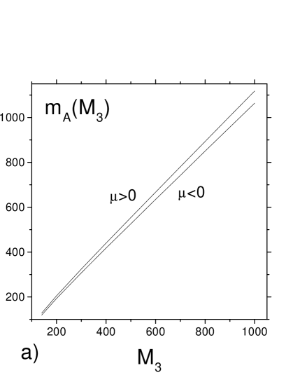
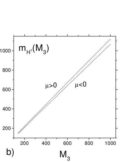
Figure 4: CP-odd (a) and charged (b) Higgs boson masses from the IR quasi-fixed points for two signs of $\mu$

In the MSSM the Higgs sector consists of five physical states: two neutral CP-even scalars $h$ and $H$, one neutral CP-odd scalar $A$, and one complex charged Higgs scalar $H^{\pm}$. At the tree level these particle masses are given by the following well-known expressions [10, 14, 25, 26, 29]:

$$m_{A}^{2} = m_{H_{1}}^{2}+m_{H_{2}}^{2}+2\mu^{2}_{tree}=m_{+}^{2}-m_{H_{2}}^{2}+2\mu^{2}_{tree}\,,$$ (16)

$$m_{H^{\pm}}^{2} = m_{A}^{2}+M_{W}^{2}\,,$$ (17)

$$m_{h,H}^{2} = \frac{1}{2}\left(M_{Z}^{2}+m_{A}^{2}\mp\sqrt{(M_{Z}^{2}+m_{A}^{2})^{2}-4M_{Z}^{2}m_{A}^{2}\cos^{2}{2\beta}}\right)\,,$$ (18)

For the CP-odd, charged and the heaviest CP-even Higgses we take the tree level expressions because the radiative corrections (including those to $\mu$) play a negligible role in this case [14, 26, 27, 28]. However, for the lightest neutral Higgs boson the radiative corrections are very important; therefore, we take them into account in the two-loop order (see [29]). These corrections depend on stop masses, trilinear soft coupling $A_{t}$ and $\mu$ calculated above.

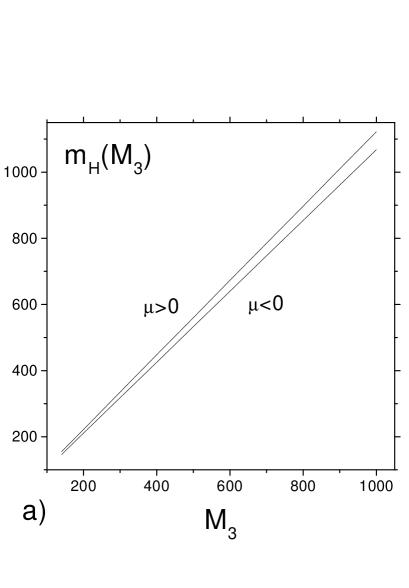
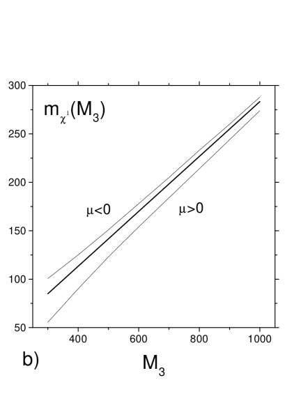
Figure 5: Heavy CP-even Higgs boson mass (a) and the chargino mass (b) from the IR quasi fixed points for two signs of $\mu$. Thick line corresponds to the limit $|\mu|\to\infty$

Using the values for $\mu^{2}$ and $\tan\beta$, we can calculate the Higgs masses as functions of the gluino mass. We recall that the fixed point values for $m_{+}^{2}$, $m_{H_{2}}^{2}$ and $\mu^{2}$ correspond to the minimum values of these parameters in the limit $Y_{0}\to\infty$. This way the lower bounds for the CP-odd, charged and heaviest CP-even Higgs boson masses as functions of $M_{3}$ are obtained. These bounds are represented in Fig. 4 and Fig. 5a respectively. As for the lightest Higgs boson, we return to it after computation of the stop masses.

Now we proceed to the lightest chargino. The mass eigenvalues for charginos are the following [14]:

$$m_{\chi_{1,2}}^{2} = \frac{1}{2}\big{[}M_{2}^{2}+\mu^{2}+2M_{W}^{2}$$ (19)

$$\mp \sqrt{(M_{2}^{2}-\mu^{2})^{2}+4M_{W}^{4}\,\cos^{2}(2\beta)+4M_{W}^{2}(M_{2}^{2}+\mu^{2}+2M_{2}\mu\,\sin(2\beta)}\big{]}\,,$$

where the weak gaugino mass is given by $M_{2}=(\tilde{\alpha}_{2}/\tilde{\alpha}_{3})M_{3}\approx 0.23M_{3}$.

We have all ingredients in eq.(19) to find the value of the lightest chargino mass as a function of $M_{3}$. The result is illustrated in Fig. 5b for different signs of $\mu$. It has already been mentioned that the IRQFP’s for $m_{+}^{2}$ and $m_{H_{2}}^{2}$ give the minimum value of $|\mu|$. We show also the lightest chargino mass in the limit $|\mu|\to\infty$ (middle line). Under the condition that $Y_{0}\gg\tilde{\alpha}_{0}$, the lightest chargino mass lies in the area between these three lines. As one can see, the preferable value of the lightest chargino mass is either its minimum or its maximum value, depending on the sign of $\mu$.

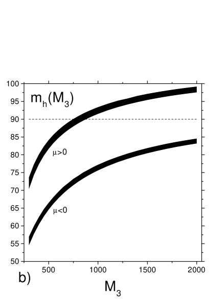
Figure 6: a) The values of the stop masses for two signs of $\mu$: $\tilde{m}_{t_{1}}$ for $\mu>0$ (a) and for $\mu<0$ (b), $\tilde{m}_{t_{2}}$ for $\mu<0$ (c) and for $\mu>0$ (d). b) The mass of the Higgs boson h for two signs of $\mu$ (shaded areas). The dashed line correspond to a minimum value of $m_{h}=90$ GeV, allowed by the experiment

Consider at last the stop masses. After diagonalization of the stop mass matrix its eigenvalues are given by the following expression [14]:

$$\tilde{m}_{t_{1,2}}^{2} = \frac{1}{2}\big{[}\tilde{m}_{t_{L}}^{2}+\tilde{m}_{t_{R}}^{2}\mp\sqrt{(\tilde{m}_{t_{L}}^{2}-\tilde{m}_{t_{R}}^{2})^{2}+4m_{t}^{2}(A_{t}-\mu\,\cot\beta)^{2}}\big{]}\,,$$ (20)

where $\tilde{m}_{t_{L}}^{2}$ and $\tilde{m}_{t_{R}}^{2}$ are given in Appendix.

The behaviour of the stop masses as functions of the gluino mass is presented in Fig. 6a. As one can see from this figure, both $\tilde{m}_{t_{1}}$ and $\tilde{m}_{t_{2}}$ are of the order of the gluino mass (more precisely they vary within the interval $0.6M_{3}-1.5M_{3}$). We want to stress that such a behaviour of the stop masses is the characteristic feature of the IRQFP scenario. On the contrary, for $m_{0}\gg m_{1/2}$ the soft parameters are far from the fixed points and the lightest stop mass squared may be arbitrary small or even negative [21, 8]. Such values of $\tilde{m}_{t_{1}}^{2}$ are not possible when fixed point values are taken. Furthermore, comparing our results with those of Refs. [8, 21], it is easy to see that the fixed point value of the lightest stop mass is very close to its maximum as a function of $M_{3}$ when the limit $Y_{0}\gg\tilde{\alpha}_{0}$ is considered. This explains why the stops are so heavy and have not been detected so far. It suffices to note that one obtains $\tilde{m}_{t_{1}}>100$ GeV when using the experimental bound on the gluino mass $M_{3}>173$ GeV. Further on we show that for the scenario at hand the lightest stop mass lies far out of the domain of LEP II when the experimental constraints on the lightest Higgs mass are taken into account.

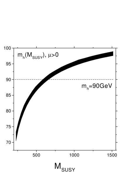
Figure 7: Dependence of the mass of the Higgs boson $h$ on $M_{SUSY}=(\tilde{m}_{t_{1}}\tilde{m}_{t_{2}})^{1/2}$ (shaded area) for $\mu>0$. The dashed line corresponds to a minimum value of $m_{h}=90$ GeV, allowed by the experiment

Now, when the masses of stops are known , we can compute the mass of the lightest Higgs boson. For this purpose we use eq.(18) together with one- and two-loop corrections [29]. The values of $\tilde{m}_{t_{1}}^{2},\tilde{m}_{t_{2}}^{2},A_{t}$ and $\mu$ that enter the expressions for one- and two-loop corrections are determined via IRQFP’s for $m^{2}_{Q},m^{2}_{U},m^{2}_{H_{2}}$ and $m^{2}_{+}$. We include also the deviations from the fixed points which are important here. As it follows from Figs.2 and 3 the fixed points for $m^{2}_{+}$ and $m^{2}_{U}$ have a very strong attraction and are reached for a wide range of initial conditions. For this reason we take the fixed point values for these masses. On the contrary, the fixed points for $m^{2}_{H_{2}}$ and $m_{Q}^{2}$ are less attractive and we take into acccount the deviations from them. In our numerical analysis we took $m^{2}_{H_{2}}/M_{3}^{2}=-0.52\div-0.40$ and $m_{Q}^{2}/M_{3}^{2}=0.69\div 0.81$. These intervals determine the uncertainty of our evaluation of the Higgs mass. The values $m^{2}_{H_{2}}/M_{3}^{2}=-0.40$ and $m_{Q}^{2}/M_{3}^{2}=0.69$ correspond to $m_{0}^{2}/m_{1/2}^{2}=0$, and the values $m^{2}_{H_{2}}/M_{3}^{2}=-0.48$ and $m_{Q}^{2}/M_{3}^{2}=0.81$ correspond to $m_{0}^{2}/m_{1/2}^{2}=2$.

Fig. 6b shows the dependence of $m_{h}$ on the gluino mass for two signs of $\mu$. The shaded areas correspond to the deviations from the fixed points discusses above. As one can see from this picture, the IRQFP scenario excludes the negative sign of $\mu$ in agreement with the conclusions made in Ref. [30] (see also discussion in the end of this section).

Further on we consider only the positive values of $\mu$. Fig. 7 shows the value of $m_{h}$ for $\mu>0$ as a function of the geometrical mean of stop masses - this parameter is often identified with a supersymmetry breaking scale $M_{SUSY}$. For $M_{SUSY}$ of the order of 1 TeV the value of the lightest Higgs mass is $m_{h}=(94.3+1.6+0.6)$ GeV, where the first uncertainty comes from the deviations from the fixed points for the mass parameters and the second one is related to that of the top-quark Yukawa coupling. This value of $m_{h}$ is calculated for the top-quark mass equal to 174.1 GeV. If one adds the uncertainty of the determination of the top-quark mass of 5.4 GeV, one finds an almost linear dependence of $m_{h}$ on $m_{t}^{pole}$. The last source of uncertainties is the value of $\alpha_{3}(M_{Z})$. If one takes the value $\alpha_{3}(M_{Z})=0.120\pm 0.005$, it gives the uncertainty in the Higgs mass of $\pm 0.4$ GeV. Finally, one has the following prediction for the lightest Higgs boson mass:

$$m_{h}=(94.3+1.6+0.6\pm 5\pm 0.4)\ \mbox{GeV},\ \ \ \mbox{ for}\ M_{SUSY}=1\ TeV.$$ (21)

One can see that the main source of uncertainty is the experimental error in the top-quark mass. As for the uncertainties connected with the fixed points, they give much smaller errors of the order of 1 GeV.

Note that the obtained result (21) is very close to the upper boundary, $m_{h}=97$ GeV, reported in Refs. [17, 31]. This means that using the IRQFP approach for all relevant SUSY breaking mass parameters, one can explain in the natural way, why the lightest Higgs boson was not detected so far. We recall that the similar result was obtained also for the lightest stop mass.

Thus, for a supersymmetry breaking scale of an order of 1 TeV the IRQFP scenario gives the lightest Higgs boson mass within the reach of LEPII. The absence of the Higgs boson events up to 100 GeV would indicate either larger values of the SUSY breaking scale or higher values of $\tan\beta$. For $M_{SUSY}>1$ TeV one has to perform a more detailed analysis of radiative corrections taking into account the running of the top mass and QCD coupling constant between the electroweak scale and SUSY scale. For higher values of $\tan\beta$ the analysis of fixed solutions becomes more complicated, due to new Yukawa couplings being involved. One may consider, of course, more radical changes like non-universality of the soft terms, new particles which appear for instance in gauge-mediated SUSY breaking models, etc.

The experimental bounds play an important role for the remaining particles as well. It has been noted already that the experimental bound on gluino mass pushes the lightest stop to be heavier than 100 GeV. The restrictions on particles masses become stronger when the experimental constraint on the lightest Higgs boson is taken into account. In the MSSM besides the Standard Model channel $e^{+}e^{-}\rightarrow hZ$ there is an additional channel for the Higgs boson production, $e^{+}e^{-}\rightarrow hA$ (see e.g. [32, 33]). The modern experimental constraint on the Higgs mass in the MSSM is $m_{h}>62.5$ GeV [35]. We have to recall, however, that the CP-odd mass has been obtained here to be larger than the Z-boson mass. This means that the Standard Model constraint on the Higgs mass $m_{h}>90$ GeV [34] can be used also for the minimal supersymmetry.

Let us see how this constraint affects the values of sparticles masses. First, one can see from Fig.7 that $\sqrt{\tilde{m}_{t_{1}}\tilde{m}_{t_{2}}}$ must be larger than 550 GeV in order the condition $m_{h}>90$ GeV to be satisfied. For the IRQFP scenario considered here this is equivalent to restriction on the gluino mass $M_{3}\geq 750$ GeV (see Figs. 6,7). Subsequently one obtains $m_{A}>844$ GeV, $m_{H^{\pm}}>846$ GeV, $m_{H}>848$ GeV, $\tilde{m}_{t_{1}}>440$ GeV for $\mu>0$. As for the lightest chargino, one has $m_{\chi_{1}}\geq 200$ GeV. Thus, these particles are too heavy to be detected in the nearest experiments.

4 Summary and Conclusion

We have analyzed the fixed point behaviour of the SUSY breaking parameters in the small $\tan{\beta}$ regime. We have made this analysis, assuming that the top quark Yukawa coupling is initially large enough to be driven at the infrared scales to its Hill-type quasi-fixed point or, equivalently, to its upper boundary value. This value of $h_{t}(M_{Z})$ corresponds to a possible Grand Unification scenario with bottom-tau unification and radiative EWSB.

We have found that solutions of RGE’s for some of the SUSY breaking parameters become insensitive to their initial values at unification scales. This is because at the infrared scales they are driven to their IR quasi-fixed points. These fixed points are used to make predictions for the masses of the Higgs bosons, stops and the lightest chargino as the functions of the only unknown parameter - the gluino mass. We have taken into account possible impact of deviations from the IR quasi-fixed points as well as experimental bounds on the gluino and the lightest Higgs masses.

For the infrared quasi-fixed point scenario the Higgs bosons except the lightest one are found to be too heavy to be accessible in the nearest experiments. The same is true for the stops and charginos. This explains in a natural way, even without knowlegde of physics at unification scale, why the stops and charginos have not been detected so far. The mass of the lightest neutral Higgs boson is also close to its upper boundary, however, for the low $\tan\beta$ case it is within the reach of LEP II.

Appendix

1. Notation [20]

$$b_{1}=11,\ b_{2}=1,\ b_{3}=-3,\ t=log\frac{M_{GUT}^{2}}{Q^{2}}$$

$$\beta_{i}=b_{i}\tilde{\alpha}_{i0},\ i=1,2,3$$

$$E(t)=(1+\beta_{3}t)^{16/(3b_{3})}(1+\beta_{2}t)^{3/b_{2}}(1+\beta_{1}t)^{13/(15b_{1})}\,,$$

$$F(t)=\int\limits_{0}^{t}E(t^{\prime})dt^{\prime}\,,$$

$$D(t)=1+6Y_{0}F(t)\,,$$

$$f_{i}(t)=\frac{1}{\beta_{i}}\left(1-\frac{1}{(1+\beta_{i}t)^{2}}\right)\,,$$

$$h_{i}(t)=\frac{t}{(1+\beta_{i}t)}\,,$$

$$e(t)=\frac{3}{2}\left[\frac{G_{1}(t)+Y_{0}G_{2}(t)}{D(t)}+\frac{(H_{2}(t)+6Y_{0}H_{4}(t))^{2}}{3D^{2}(t)}+H_{8}(t)\right]\,,$$

$$\bar{e}(t)=\frac{G_{2}(t)}{4F(t)}+\frac{H_{4}^{2}(t)}{2F^{2}(t)}+\frac{3H_{8}(t)}{2}\,,$$

$$f(t)=-\frac{6Y_{0}H_{3}(t)}{D^{2}(t)}\,,$$

$$h(t)=\frac{1}{2}\left(\frac{3}{D(t)}-1\right)\,,$$

$$k(t)=\frac{3Y_{0}F(t)}{D^{2}(t)}\,,$$

$$H_{2}(t)=\left(\frac{16}{3}\tilde{\alpha}_{30}h_{3}(t)+3\tilde{\alpha}_{20}h_{2}(t)+\frac{13}{15}\tilde{\alpha}_{10}h_{1}(t)\right)\,,$$

$$H_{3}(t)=tE(t)-F(t)\,,$$

$$H_{4}(t)=F(t)H_{2}(t)-H_{3}(t)\,,$$

$$H_{5}(t)=\left(-\frac{16}{3}\tilde{\alpha}_{30}f_{3}(t)+\tilde{\alpha}_{20}6f_{2}(t)-\frac{22}{15}\tilde{\alpha}_{10}f_{1}(t)\right)\,,$$

$$H_{6}(t)=\int\limits_{0}^{t}H_{2}^{2}(t^{\prime})E(t^{\prime})dt^{\prime}\,,$$

$$H_{7}(t)=\left(3\tilde{\alpha}_{20}h_{2}(t)+\frac{3}{5}\tilde{\alpha}_{10}h_{1}(t)\right)\,,$$

$$H_{8}(t)=\left(-\frac{8}{3}\tilde{\alpha}_{30}f_{3}(t)+\tilde{\alpha}_{20}f_{2}(t)-\frac{1}{3}\tilde{\alpha}_{10}f_{1}(t)\right)\,,$$

$$G_{1}(t)=F_{2}(t)-\frac{1}{3}H_{2}^{2}(t)\,,$$

$$G_{2}(t)=6F_{3}(t)-F_{4}(t)-4H_{2}(t)H_{4}(t)+2F(t)H_{2}^{2}(t)-2H_{6}(t)\,,$$

$$F_{2}(t)=\left(\frac{8}{3}\tilde{\alpha}_{30}f_{3}(t)+\frac{8}{15}\tilde{\alpha}_{10}f_{1}(t)\right)\,,$$

$$F_{3}(t)=F(t)F_{2}(t)-\int\limits_{0}^{t}E(t^{\prime})F_{2}(t^{\prime})dt^{\prime}\,,$$

$$F_{4}(t)=\int\limits_{0}^{t}E(t^{\prime})H_{5}(t^{\prime})dt^{\prime}\,,$$

2. Solutions of the RGE’s for supersymmetry breaking parameters [14, 20]

$$A_{t}(t)=\frac{A_{t}(0)}{1+6Y_{0}F(t)}-m_{1/2}\left(H_{2}-\frac{6Y_{0}H_{3}}{1+6Y_{0}F(t)}\right)\,,$$

$$m_{H_{1}}^{2} = m_{0}^{2}+m_{1/2}^{2}\left(\frac{3}{2}\tilde{\alpha}_{20}f_{2}(t)+\frac{3}{10}\tilde{\alpha}_{10}f_{1}(t)\right)\,,$$

$$m_{H_{2}}^{2} = m_{1/2}^{2}e(t)+A_{t}(0)m_{1/2}f(t)+m_{0}^{2}h(t)-k(t)A_{t}(0)^{2}\,,$$

$$m_{Q}^{2}(t)=\frac{2}{3}m_{0}^{2}+\frac{1}{3}m_{H_{2}}^{2}+m_{1/2}^{2}(\frac{8}{3}\tilde{\alpha}_{30}f_{3}(t)+\tilde{\alpha}_{30}f_{2}(t)-\frac{1}{15}\tilde{\alpha}_{10}f_{1}(t))$$

$$m_{U}^{2}(t)=\frac{1}{3}m_{0}^{2}+\frac{2}{3}m_{H_{2}}^{2}+m_{1/2}^{2}(\frac{8}{3}\tilde{\alpha}_{30}f_{3}(t)-\tilde{\alpha}_{20}\frac{1}{2}f_{2}(t)-\frac{13}{30}\tilde{\alpha}_{10}f_{1}(t))$$

The parameters $\tilde{m}_{t_{L}}^{2}$ and $\tilde{m}_{t_{R}}^{2}$ are connected with $m_{Q}^{2}$ and $m_{U}^{2}$ by the following relations:

$$\tilde{m}_{t_{R}}^{2} = m_{U}^{2}+m_{t}^{2}+M_{Z}^{2}\cos{2\beta}(\frac{2}{3}\sin^{2}{\theta_{W}})$$

$$\tilde{m}_{t_{L}}^{2} = m_{Q}^{2}+m_{t}^{2}-M_{Z}^{2}\cos{2\beta}(\frac{2}{3}\sin{\theta_{W}}-\frac{1}{2})$$

3. One-loop corrections to the parameter $\mu$ [14]

$$\Delta_{Z} = \frac{3g_{2}^{2}}{32\pi^{2}}\frac{m_{t}^{2}}{M_{W}^{2}\cos^{2}{\beta}}[b(\tilde{m}_{t_{1}}^{2})+b(\tilde{m}_{t_{2}}^{2})+2m_{t}^{2}+$$

$$+ (A_{t}^{2}-\mu^{2}\cot^{2}{\beta})\frac{b(\tilde{m}_{t_{1}}^{2})-b(\tilde{m}_{t_{2}}^{2})}{\tilde{m}_{t_{1}}^{2}-\tilde{m}_{t_{2}}^{2}}]$$

where $b(m)=m^{2}(\log\frac{m^{2}}{m_{t}^{2}}-1)$

Acknowledgments

We are grateful to W. de Boer, K.A.Ter-Martirosian and R.B.Nevzorov for useful discussions. Financial support from RFBR grant # 96-02-17379 is kindly acknowledged. Also this work was partially supported by INTAS under the Contract INTAS-96-155. One of the authors (G. Y.) is thankful to the Joint Institute for Nuclear Research (Dubna) where this work has been started, for a hospitality.

References

-
[1]
H. P. Nilles, Phys. Rep. 110 (1984) 1,
H. E. Haber and G. L. Kane, Phys. Rep. 117 (1985) 75;
A.B. Lahanas and D.V. Nanopoulos, Phys. Rep. 145 (1987) 1;
R. Barbieri, Riv. Nuo. Cim. 11 (1988) 1;
W. de Boer, Progr. in Nucl. and Particle Phys., 33 (1994) 201;
D.I. Kazakov, Surveys in High Energy Physics, 10 (1997) 153. - [2] B. Pendleton and G. Ross, Phys. Lett. B98 (1981) 291.
- [3] B. Schrempp, F.Schrempp, Phys. Lett. B299 (1993) 321.
- [4] B. Schrempp, Phys. Lett. B344 (1995) 193
- [5] B. Schrempp, M. Wimmer, Progr. Part. Nucl. Phys. 37 (1996) 1
- [6] C. T. Hill, Phys. Rev. D24 (1981) 691.
-
[7]
E. Paschos, Z. Phys. C26 (1984) 235;
J. Halley, E. Paschos, H. Usler, Phys. Lett. B155(1985) 107. -
[8]
J. Bagger, S. Dimopoulos, E. Masso, Nucl. Phys. B253
(1985) 397 ;
J. Bagger, S. Dimopoulos, E. Masso, Phys. Lett. B156 (1985) 357 ;
S. Dimopoulos, S. Theodorakis, Phys. Lett B154 (1985) 153 - [9] W. Barger, M. Berger, P. Ohman, Phys. Lett. B314 (1993) 351
- [10] P. Langacker, N. Polonsky, Phys. Rev. D49 (1994) 454
- [11] M. Carena et al, Nucl. Phys. B419 (1994) 213
- [12] W. Bardeen et al, Phys. Lett. B320 (1994) 110.
- [13] M. Jones, for the CDF and D0 Coll., talk at the XXXIIIrd Recontres de Moriond, (Electroweak Interactions and Unified Theories), Les Arcs, France, March 1998;
- [14] W. de Boer et al., Z. Phys C67 (1995) 647.
- [15] P. Nath et al., Phys. Rev. D52 (1995) 4169.
- [16] M. Carena, C. E. M. Wagner, Nucl. Phys. B452 (1995) 45.
- [17] J. Casas, J. Espinosa, H. Haber, Nucl. Phys. B526 (1998) 3.
- [18] M. Lanzagorta, G. Ross, Phys. Lett. B364 (1995) 163.
- [19] S. A. Abel, B. C. Allanach Phys. Lett. B415 (1997) 371.
- [20] L. Ibanez, C. Lopez, Phys. Lett B126 (1983) 54; Nucl. Phys. B233(1984) 511, Nucl. Phys. B256 (1985) 218.
- [21] E. G. Floratos, G. K. Leontaris, Nucl. Phys. B452 (1995) 471
- [22] W. de Boer et al., hep-ph/9712376, Proc. of Int. Europhysics Conference on High Energy Physics (HEP 97), Jerusalem, Israel, August 1997.
- [23] D. M. Pierce, J. A. Bagger, K. Matchev and R. Zhang, Nucl. Phys. B491 (1997) 3.
- [24] C. Caso et al. (Particle Data Group), The European Physical Journal C3 (1998) 1.
- [25] J. Ellis, G. Ridolfi, F. Zwirner, Phys. Lett. Phys. Lett. B257 (1991) 83
- [26] J. Ellis, G. Ridolfi, F. Zwirner, Phys. Lett. B262 (1991) 477.
- [27] A. Brignole et al, Phys. Lett. B271 (1991) 123.
- [28] Z. Kunszt, F. Zwirner, Nucl. Phys. B385 (1992) 3
- [29] M. Carena, M. Quiros, C.E.M. Wagner, Nucl. Phys. B461 (1996) 407.
- [30] W. de Boer, H-J. Grimm, A. Gladyshev and D. Kazakov, Phys.Lett. B438 (1998) 281; hep-ph/9805378.
- [31] A.Gladyshev, D.Kazakov, W. de Boer, D. Burkart, R.Ehret, Nucl. Phys. B498 (1997) 3.
- [32] The ALEPH Collaboration, CERN-PPE/98-145.
- [33] The OPAL Collaboration, CERN-PPE/98-173.
- [34] The OPAL Collaboration, CERN-PPE/98-093.
- [35] C. Caso et al., Eur.Phys.J. C3 (1998) 1.