Chiral Phase Transition of QCD at Finite Temperature and Density from Schwinger-Dyson Equation

Abstract

We study the chiral phase transition of QCD at finite temperature and density by numerically solving Schwinger-Dyson equation for the quark propagator with the improved ladder approximation in the Landau gauge. Using the solution we calculate a pion decay constant from a generalized version of Pagels-Stokar formula. Chiral phase transition point is determined by analyzing an effective potential for the quark propagator. We find solutions for which chiral symmetry is broken while the value of the effective potential is larger than that for the chiral symmetric vacuum. These solutions correspond to meta-stable states, and the chiral symmetric vacuum is energetically favored. We present a phase diagram on the general temperature–chemical potential plane, and show that phase transitions are of first order in wide range.

I Introduction

In QCD an approximate chiral symmetry exists at the Lagrangian level and it is spontaneously broken by the strong gauge interaction. Accordingly approximate Nambu-Goldstone (NG) bosons appear, and pions are regarded as the NG bosons. In hot and/or dense matter, however, quark condensates melt at some critical point, and the chiral symmetry is restored (for recent reviews, see, e.g., Ref. [1]). To study the chiral phase transition we need non-perturbative treatment.

Schwinger-Dyson Equation (SDE) is a powerful tool for studying the qualitative structure of chiral symmetry breaking of QCD. By suitable choices of the running coupling, in which the asymptotic freedom is incorporated, the SDE provides a non-trivial solution for the mass function. The behavior of the mass function at high energy is consistent with that given by the operator product expansion technique (for a review, see, e.g., Ref. [2]). The SDE is understood as a stationary condition of an effective potential for the quark propagator, and the chiral broken solution is energetically favored by the effective potential[3, 4, 5, 6].

The SDE was applied for studying the chiral phase transition of QCD at finite temperature and/or density [7, 8, 9, 10, 11, 12, 13, 14, 15, 16, 17, 18]. In many of those the chiral phase transition point was determined from the point where the mass function (or pion decay constant) vanished without studying an effective potential. In Ref. [13] an effective potential for the mass function was analyzed by using an approximate form of momentum dependence of the mass function. It was shown that there were meta-stable states where the chiral symmetry was broken while the energy was bigger than that for the symmetric vacuum. It is interesting to study whether this kind of meta-stable state is derived by fully solving the SDE.

In this paper we study the chiral phase transition in QCD at finite temperature and/or density by numerically solving the SDE using Matsubara formalism. As an order parameter we calculate a pion decay constant using a generalized version of Pagels-Stokar formula [19]. We calculate the value of the effective potential at the solution of the SDE to determine the chiral phase transition points. We show that meta-stable states actually exist in wide range. The order of phase transition are determined by comparing the order parameter with the effective potential. The phase transition is of the first order for wide range at $T\neq 0$ and $\mu\neq 0$.

This paper is organized as follows. An effective potential for the quark propagator is introduced at finite temperature and/or density in section II. The SDE is derived as a stationary condition of the potential. In section III a formula for calculating a pion decay constant is presented. Section IV is a main part of this paper, where numerical solutions of the SDE are shown. Values of the pion decay constant and the effective potential are calculated from the solutions, and the phase structure is studied. Finally a summary and discussion are given in section V.

II Effective Potential and Schwinger-Dyson Equation

At zero temperature the effective action for the quark propagator $S_{F}$ is given by [4, 6]

$$\Gamma[S_{F}]=i\mbox{Tr}\,\mbox{Ln}\,S_{F}-\mbox{Tr}\left[i\partial\kern-5.5pt\mbox{\it/}S_{F}\right]-i\kappa_{\rm 2PI}[S_{F}]\ ,$$ (1)

where $\kappa_{\rm 2PI}$ stands for the two particle irreducible (with respect to quark-line) diagram contribution. In this paper we take the first order approximation for $\kappa_{\rm 2PI}$, in which one gluon exchange graph contribute,

$$\kappa_{\rm 2PI}[S_{F}]=-\frac{N_{\rm f}N_{\rm C}C_{2}}{2}\int d^{4}xd^{4}yg^{2}\mbox{tr}\,\left[S_{F}(x-y)i\gamma_{\mu}S_{F}(y-x)i\gamma_{\nu}\right]D^{\mu\nu}(x-y)\ ,$$ (2)

where the number of flavor ($N_{\rm f}$) and of color ($N_{\rm C}$) and the second Casimir of SU($N_{\rm C}$) ($C_{2}$) appear since we factor color and flavor indices from the quark and gluon propagators. In this expression, the quark propagator $S_{F}$ carries bispinor indices and the gluon propagator $D^{\mu\nu}$ carries Lorenz indices. From the above effective action the effective potential for $S_{F}$ is obtained by the usual procedure. In momentum space it is expressed as

$$V[S_{F}] = \int\frac{d^{4}p}{i(2\pi)^{4}}\left\{\mbox{\rm ln}\,\mbox{\rm det}\,\left[S_{F}(p)\right]+\mbox{\rm tr}\,\left[p\kern-5.5pt\mbox{\it/}iS_{F}(p)\right]\right\}$$ (4)

$$+\frac{1}{2}\int\frac{d^{4}p}{i(2\pi)^{4}}\int\frac{d^{4}k}{i(2\pi)^{4}}C_{2}g^{2}(p,k)\mbox{\rm tr}\,\left[iS_{F}(p)\gamma_{\mu}iS_{F}(k)\gamma_{\nu}\right]iD^{\mu\nu}(k-p)\ ,$$

where an overall factor $N_{\rm C}N_{\rm f}$ is dropped. The running coupling $g^{2}(p,k)$ is introduced to improve Schwinger–Dyson Equation (SDE) to include aymptotic freedom of QCD. An explicit form of the running coupling will be given below. In this paper we take the Landau gauge for the gluon propagator:

$$iD^{\mu\nu}(l)=\frac{1}{l^{2}}\left[g^{\mu\nu}-\frac{l^{\mu}l^{\nu}}{l^{2}}\right]\ .$$ (5)

General form of the full quark propagator is expressed as

$$iS_{F}^{-1}(p)=A(p)p\kern-5.5pt\mbox{\it/}-B(p)\ .$$ (6)

SDE for the quark propagator $S_{F}$ is given as a stationary condition of the above effective potential[4] (See also, Ref. [6]). The SDE gives coupled equations for $A$ and $B$. If the running coupling $g(p,k)$ is a function in $p^{2}$ and $k^{2}$, i.e., it does not depend on $p\cdot k$, it is easy to show that $A(p^{2})=1$ is a solution of the SDE in the Landau gauge with the ladder approximation.

Let us go to non-zero temperature and density. In the imaginary time formalism[20] the partition function is calculated by the action given by (See, for reviews, e.g., Refs. [21, 22].)

$$S=\int^{1/T}_{0}d\tau\int d^{3}x\left[{\cal L}_{\rm QCD}+\mu\overline{\psi}\gamma^{0}\psi\right]\ ,$$ (7)

where $T$ and $\mu$ denote temperature and chemical potential associated with quark (baryon) number density, and ${\cal L}_{\rm QCD}$ takes the same form as QCD Lagrangian at $T=\mu=0$. From the above action we obtain an effective potential for the quark propagator $S_{F}$ similar to the one in Eq. (4):

$$V[S_{F}]=T\sum_{u}\int\!\frac{d^{3}\vec{p}}{(2\pi)^{3}}\left\{\mbox{\rm ln}\,\mbox{\rm det}\,\left[S_{F}(p)\right]+\mbox{\rm tr}\,\left[p\kern-5.5pt\mbox{\it/}iS_{F}(p)\right]\right\}$$ (9)

$$+\frac{1}{2}T^{2}\sum_{u,v}\int\!\frac{d^{3}\vec{p}}{(2\pi)^{3}}\int\!\frac{d^{3}\vec{k}}{(2\pi)^{3}}C_{2}g^{2}(p,k)\,\mbox{\rm tr}\left[iS_{F}(p)\gamma_{\mu}iS_{F}(k)\gamma_{\nu}\right]iD^{\mu\nu}(k-p)\ ,$$

where

$$p_{0}=iu+\mu\ ,\quad u=(2m+1)\pi T\ ,$$ (10)

$$k_{0}=iv+\mu\ ,\quad v=(2n+1)\pi T\ ,\quad(n,m=\mbox{\rm integer})\ ,$$ (11)

and $\sum_{u}$ and $\sum_{v}$ imply summations over $m$ and $n$, respectively.

Argument of the running coupling should be taken as $(k-p)^{2}$ for preserving the chiral symmetry [23]. However, as is shown in Ref. [23], angular average, i.e., the running coupling is a function in $-p_{0}^{2}+|\vec{p}|^{2}-k_{0}^{2}+|\vec{k}|^{2}$, is a good approximation at $T=\mu=0$. If we naively extend this approximation, the running coupling will depend on $\mu$. However, the running coupling should not depend on $\mu$. Then in this paper we use the approximation where the running coupling is a function in $-(p_{0}-\mu)^{2}+|\vec{p}|^{2}-(k_{0}-\mu)^{2}+|\vec{k}|^{2}$. The explicit form of the running coupling is [24]

$$g^{2}(p,k) = \left(4\pi\right)^{2}\frac{3}{11N_{\rm C}-2N_{\rm f}}\,\overline{\lambda}\left(\mbox{ln}\left(\frac{u^{2}+x^{2}+v^{2}+y^{2}}{\Lambda_{\rm qcd}^{2}}\right)\right)\ ,$$ (12)

$$\overline{\lambda}(t) = \left\{\begin{array}[]{ll}\displaystyle\frac{1}{t}&\mbox{if}\ t_{\rm F}<t\\ \displaystyle\frac{1}{t_{\rm F}}+\frac{\left(t_{\rm F}-t_{\rm C}\right)^{2}-\left(t-t_{\rm C}\right)^{2}}{2t_{\rm F}^{2}\left(t_{\rm F}-t_{\rm C}\right)}&\mbox{if}\ t_{\rm C}<t<t_{\rm F}\\ \displaystyle\frac{1}{t_{\rm F}}+\frac{\left(t_{\rm F}-t_{\rm C}\right)}{2t_{\rm F}^{2}}&\mbox{if}\ t<t_{\rm C}\\ \end{array}\right.\ ,$$ (16)

with

$$x\equiv|\vec{p}|\ ,\ \ y\equiv|\vec{k}|\ .$$ (17)

$\Lambda_{\rm qcd}$ is a scale where the one-loop running coupling diverges, and the value of $\Lambda_{\rm qcd}$ will be determined later from the infrared structure of the present analysis. $t_{\rm F}$ and $t_{\rm C}$ are parameters introduced to regularize the infrared behavior of the running coupling. In the numerical analysis below, since the dominant part of the mass function lies below the threshold of charm quark, we will take $N_{\rm f}=3$ and $N_{\rm C}=3$. Moreover, we use fixed values $t_{\rm F}=0.5$ and $t_{\rm C}=2.0$ [2].

General form of the full quark propagator, which is invariant under the Parity-transformation, is given by[7, 11, 12, 15]

$$iS_{\rm F}^{-1}(p)=A(p)p\kern-5.5pt\mbox{\it/}-B(p)+C(p)p_{0}\gamma^{0}-\frac{i}{2}\left[\gamma^{0}\,,\,p\kern-5.5pt\mbox{\it/}\right]\,D(p)\ .$$ (18)

Here $A$ $\sim$ $D$ are functions in $p_{0}$ and $|\vec{p}|$ (as well as $T$ and $\mu$), although we write $A(p)$, etc.

It should be noticed that the effective potential in Eq. (9) is invariant under the tranfromation:

$$S_{F}(p_{0},\vec{p})\longrightarrow S_{F}^{\prime}(p_{0},\vec{p})=\left(i\gamma^{1}\gamma^{3}\gamma^{0}\right)S_{F}^{T}(p_{0},-\vec{p})\left(i\gamma^{0}\gamma^{1}\gamma^{3}\right)\ ,$$ (19)

where $S_{F}^{T}$ implies transposition of $S_{F}$ in spinor space. At $T=\mu=0$ this is nothing but the time reversal symmetry. It is natural to expect that this “time reversal” symmetry is not spontaneously broken. Existence of this “time reversal” leads $D(p)=0$.

Moreover, at $\mu=0$ the effective potential is invariant under the following “charge conjugation”:

$$S_{F}(p)\longrightarrow S_{F}^{\prime}(p)=-(i\gamma^{2}\gamma^{0})S_{F}^{T}(-p)(i\gamma^{2}\gamma^{0})\ .$$ (20)

We also assume this symmetry is not spontaneously broken, and it implies that all the scalar functions $A$, $B$ and $C$ (as well as $D$) are even functions in $p_{0}=iu$. As we mentioned above, at $T=\mu=0$, of course $C(p)=0$, and $A(p)=1$ in the Landau gauge. $C(p)\neq 0$ as well as $A(p)\neq 1$ does not imply chiral symmetry breaking, and non-zero $B(p)$ is the only signal of the breaking in the present analysis. Then we consider $A(p)-1=C(p)=0$ as an approximate solution at general $T$ and $\mu$. We note that non-zero $D(p)$ also breaks chiral symmetry, however this term do not contribute to local order parameter of ciral symmetry, $\langle\overline{\psi}\psi\rangle=-\int\mbox{tr}S_{F}$. We choose vacuum of “time reversal” invariance as discussed above.

As in the case at $T=\mu=0$, the SDE is given as a stationary condition of the effective potential (9):

$$iS_{\rm F}^{-1}(p)-p\kern-5.5pt\mbox{\it/}=T\sum_{v}\int\frac{d^{3}\vec{k}}{\left(2\pi\right)^{3}}C_{2}g^{2}(p,k)\gamma_{\mu}iS_{\rm F}(k_{f})\gamma_{\nu}iD^{\mu\nu}(k-p)\ .$$ (21)

By taking a trace and performing the three-dimensional angle integration (Note that the present form of the running coupling does not depend on the angle.), we obtain a self-consistent equation for $B$:

$$B(p)=K(p,k)\ast\frac{B(k)}{B^{2}(k)-k^{2}}\equiv T\sum_{v}\int\frac{dyy^{2}}{2\pi^{2}}K(p,k)\frac{B(k)}{B^{2}(k)-k^{2}}\ ,$$ (22)

where

$$K(p,k)\equiv\frac{3}{2}C_{2}g^{2}(p,k)\times\frac{1}{2xy}\ln\left(\frac{(u-v)^{2}+(x+y)^{2}}{(u-v)^{2}+(x-y)^{2}}\right)\ .$$ (23)

In general cases $B$ is a complex function. By using the fact that $K(p,k)$ is a real function, it is easily shown that $B^{\ast}(p)$ satisfies the same equation as $B(p^{\ast})$ does, where $p^{\ast\mu}=(p^{0\ast},\vec{p})=(-iu+\mu,\vec{p})$. So these two are equal to each other up to sign, $B^{\ast}(p)=B(p^{\ast})$ or $B^{\ast}(p)=-B(p^{\ast})$. Since $B$ is an even function in $p_{0}$ at $\mu=0$, the choice of positive (negative) sign implies that $B$ is real (pure imaginary) at $\mu=0$. $B$ should be real at $\mu=0$, then

$$B^{\ast}(p)=B(p^{\ast})\ .$$ (24)

After a solution of the SDE (21) is substituted with the approximate solution $A(p)-1=C(p)=0$ into Eq. (9), the effective potential becomes

$$\overline{V}[B_{\rm sol}] \equiv V[B_{\rm sol}]-V[B=0]$$ (25)

$$= \frac{2}{\pi^{2}}T\sum_{u}\int dxx^{2}\left[-\ln\left(\frac{B^{2}_{\rm sol}(p)-p^{2}}{-p^{2}}\right)+\frac{B^{2}_{\rm sol}(p)}{B^{2}_{\rm sol}(p)-p^{2}}\right]\ ,$$ (26)

where $B_{\rm sol}$ denotes a solution of Eq. (22). This value of the effective potential is understood as the energy density of the solution. So the true vacuum should be determined by studying the value of the effective potential. When the value of $\overline{V}[B_{\rm sol}]$ for a nontrivial solution $B_{\rm sol}$ is negative, the chiral broken vacuum is energetically favored. Positive $\overline{V}[B_{\rm sol}]$, however, implies that the chiral symmetric vacuum is the true vacuum.

III Pion Decay Constant

At zero temperature and zero chemical potential the pion decay constant is defined by the matrix element of the axial-vector current between the vacuum and one-pion state:

$$\langle 0|J_{5\mu}^{a}(0)|\pi^{b}(q)\rangle=i\delta^{ab}q_{\mu}f_{\pi}\ ,$$ (27)

where $a$ and $b$ denote iso-spin indices and $J_{5\mu}^{a}=\overline{\psi}\gamma_{\mu}\gamma_{5}T^{a}\psi$ is an axial-vector current with $T^{a}$ being a generator of SU($N_{\rm f}$). At finite temperature and density there are two distinct pion decay constant[25] according to space-time symmetry of matirix element,which are defined by

$$\langle 0|J_{5\mu}^{a}(0)|\pi^{b}(q)\rangle_{T,\mu}=i\delta^{ab}\left[V_{\mu}(V\cdot q)f_{\pi L}+(g_{\mu\nu}-V_{\mu}V_{\nu})q^{\nu}f_{\pi T}\right]\ ,$$ (28)

where $V^{\mu}=(1,\vec{0})$ is a vector of medium. In this expression $f_{\pi L}$ and $f_{\pi T}$ are defined in the zero momentum limit, $q\rightarrow 0$ [25].

The above pion decay constants are expressed by using the amputated pion BS amplitude $\hat{\chi}$ as

$$V_{\mu}(V\cdot q)f_{\pi L}+(g_{\mu\nu}-V_{\mu}V_{\nu})q^{\nu}f_{\pi T}$$ (29)

$$\qquad=-\frac{N_{\rm C}}{2}T\sum_{u}\int\frac{d^{3}p}{(2\pi)^{3}}\mbox{tr}\,\left[\gamma_{\mu}\gamma_{5}iS_{F}(p+q/2)\hat{\chi}(p;q)iS_{F}(p-q/2)\right]\ .$$ (30)

By using the current conservation, it is shown that the pion momentum $\vec{q}$ and the pion energy $q_{0}$ satisfy the dispersion relation [25]

$$q_{0}^{2}=\frac{f_{\pi T}}{f_{\pi L}}\left|\vec{q}\right|^{2}\ .$$ (31)

It is straightforward to obtain the pion decay constant if we have explicit expresstion of the amputated pion BS amplitude. Although it is generally quite difficult to obtain the BS amplitude, one can determine it in $q\rightarrow 0$ limit, $\hat{\chi}(p;q=0)$, from the chiral Ward-Takahashi identity

$$iq^{\mu}\Gamma_{5\mu}^{a}\left(p-q/2,p+q/2\right)=S_{F}^{-1}\left(p-q/2\right)T_{a}\gamma_{5}+T_{a}\gamma_{5}S_{F}^{-1}\left(p+q/2\right)\ ,$$ (32)

where $\Gamma_{5\mu}^{a}$ is the axial vector–quark–antiquark vertex function, and we have suppressed color indices. (Note that $q^{0}$ in Eq. (32) is independent of $\vec{q}$, i.e., they do not generally satisfy the pion on-shell dispersion relation (31).) In the zero momentum limit, $\vec{q}$, $q^{0}\rightarrow 0$ (the on-shell limit of the pion), $\Gamma_{5\mu}^{a}$ is dominated by the pion-exchange contribution:

$$i\Gamma_{5\mu}^{a}\left(p-q/2,p+q/2\right)\mathop{\longrightarrow}_{\vec{q},q^{0}\rightarrow 0}i\left[V_{\mu}(V\cdot q)f_{\pi L}+(g_{\mu\nu}-V_{\mu}V_{\nu})q^{\nu}f_{\pi T}\right]\frac{1}{q_{0}^{2}-\omega_{q}^{2}}\hat{\chi}(p,0)T_{a}\ ,$$ (33)

where $\omega_{q}^{2}=\left(f_{\pi T}/f_{\pi L}\right)|\vec{q}|^{2}$. Substituting Eq. (33) into Eq. (32) and taking the zero momentum limit, we find

$$\hat{\chi}(p;0)=\frac{2}{f_{\pi L}}B(p)\gamma_{5}\ ,$$ (34)

where we have used $D(p)=0$ in $S_{F}(p)$.

The approximation adopted by Pagels and Stokar [19] is essentially neglecting derivatives of $\hat{\chi}$ in the zero momentum limit (See, for reviews, e.g., Refs. [2, 26]):

$$\lim_{\vec{q}\rightarrow 0}\frac{\partial}{\partial|\vec{q}|}\hat{\chi}(p;q)=\lim_{\vec{q}\rightarrow 0}\frac{\partial}{\partial q_{0}}\hat{\chi}(p;q)=0\ .$$ (35)

This approximation is same as replacing $\hat{\chi}(p;q)$ in Eq. (30) with $\hat{\chi}(p;0)$, and reproduces the exact value of $f_{\pi}$ at $T=0$ in the ladder approximation within a small error [2]. Then we use the same approximation at finite $T$ and $\mu$ in this paper. Replacing $\hat{\chi}(p;q)$ with $\hat{\chi}(p;0)$ in Eq. (30), differentiating Eq. (30) with respect to $q^{\alpha}$ and taking $q\rightarrow 0$ limit, we obtain

$$i\delta^{ab}[V_{\mu}V_{\alpha}f_{\pi L}+(g_{\mu\alpha}-V_{\alpha}V_{\mu})f_{\pi}]$$ (36)

$$\hskip 14.22636pt=-\frac{N_{\rm C}}{2}T\sum_{u}\int\frac{d^{3}p}{(2\pi)^{3}}\mbox{tr}\,\Biggl{[}\gamma_{\mu}\gamma_{5}\left\{\frac{i}{2}\frac{S_{F}(p)}{\partial p^{\alpha}}\hat{\chi}(p;0)iS_{F}(p)+iS_{F}(p)\hat{\chi}(p;0)\frac{i}{2}\frac{S_{F}(p)}{\partial p^{\alpha}}\right\}\Biggr{]}\ .$$ (37)

Here we have incorporated the on-shell dispersion relation (31). Then substituting Eq. (34) into Eq. (37) and taking $V_{\mu}V_{\alpha}$ part, we find

$$f_{\pi L}^{2}=4N_{\rm C}T\sum_{u}\int\frac{dxx^{2}}{2\pi^{2}}\frac{B(p)\left(B(p)-p_{0}\frac{\partial B(p)}{\partial p_{0}}\right)}{\left(B^{2}(p)-p^{2}\right)^{2}}\ ,$$ (38)

where we performed the three-dimensional angle integration. If the mass function $B(p)$ is a function in $p^{2}=p_{0}^{2}-\vec{p}^{2}$, this agrees with the formula derived in Ref. [14]. We also obtain a similar formula for $f_{\pi T}$ by selecting the $(g_{\mu\alpha}-V_{\mu}V_{\alpha})$ part:

$$f_{\pi T}f_{\pi L}=4N_{\rm C}T\sum_{u}\int\frac{dxx^{2}}{2\pi^{2}}\frac{B(p)\left(B(p)-\frac{x}{3}\frac{\partial B(p)}{\partial x}\right)}{\left(B^{2}(p)-p^{2}\right)^{2}}\ ,$$ (39)

where $f_{\pi L}$ in the left hand side appears from the normalization of $\hat{\chi}$ (see Eq. (34)).

It is convenient to define a space-time averaged pion decay constant by

$$f_{\pi}^{2} \equiv f_{\pi L}\frac{1}{4}g^{\mu\alpha}\frac{\partial}{\partial q^{\alpha}}\left(V_{\mu}(V\cdot q)f_{\pi L}+(g_{\mu\nu}-V_{\mu}V_{\nu})q^{\nu}f_{\pi T}\right)$$ (40)

$$= \frac{1}{4}\left(f_{\pi L}^{2}+3f_{\pi T}f_{\pi L}\right)\ .$$ (41)

This expression aggrees with Pagels-Stokar formula [19] at $T=0$ and $\mu=0$ after replacing the integral variables.

In the formula (38) we need a derivative of $B(p)$ with respect to $p_{0}$. However what is obtained by solving the SDE (22) is a function in discrete $u=(2n+1)\pi T$. To obtain the derivative an “analytic continuation” in $u$ from discrete variable to continuous variable is needed. This “analytic continuation” is done by using the SDE (22) itself:

$$p_{0}\frac{\partial B(p)}{\partial p_{0}}=p_{0}\frac{\partial K(p,k)}{\partial p_{0}}\ast\frac{B(k)}{B^{2}(k)-k^{2}}\ .$$ (42)

IV Numerical Analysis

In this section we will numerically solve the SDE (22) and calculate the effective potential and the pion decay constant $f_{\pi}(T)$ defined in Eq. (41) for the cases 1) $T=0$ and $\mu\neq 0$, 2) $T\neq 0$ and $\mu=0$ and 3) $T\neq 0$ and $\mu\neq 0$, separately. The essential parameters in the present analysis are $\Lambda_{\rm qcd}$ and $t_{F}$ in the running coupling (16). In this paper we fix $t_{\rm F}=0.5$ and the value of $\Lambda_{\rm qcd}$ is determined by calculating the pion decay constant through the Pagels-Stokar formula [19] at $T=\mu=0$. Most results are presented by the ratio to the pion decay constant at $T=\mu=0$. When we present actual values, we use the value of the pion decay constant in the chiral limit, $f_{\pi}=88$ MeV [27]. (This value of $f_{\pi}$ yields $\Lambda_{\rm qcd}\simeq 582$ MeV.)

A Preliminary

Here we will summarize the framework of the numerical analysis done below. Variables $x$ and $y$ in Eq. (17) take continuous values from $0$ to $\infty$. To solve the SDE numerically we first introduce new variables $X$ and $Y$ as $X\equiv\ln(x/\Lambda_{\rm qcd})$ and $Y\equiv\ln(y/\Lambda_{\rm qcd})$. These variables take values from $-\infty$ to $\infty$. Dominant contributions to the decay constant and the effective potential lie around $0$, i.e., $x$ or $y$ is around $\Lambda_{\rm qcd}$, as shown later. Then we introduce ultraviolet and infrared cutoffs, $X,Y\in[\lambda_{\rm IR},\lambda_{\rm UV}]$. Finally, we descretize $X$ and $Y$ at $N_{X}$ points evenly:

$$X_{i},Y_{i} = \lambda_{\rm IR}+\Delta X\cdot i\ ,\qquad i=0,1,\ldots,N_{X}-1\ ,$$ (44)

$$\Delta X=\frac{\lambda_{\rm UV}-\lambda_{\rm IR}}{N_{X}-1}\ .$$

Accordingly integrations over $x$ and $y$ are replaced with appropriate summations

$$\int dx\,,\ \int dy\ \rightarrow\ \Delta X\sum_{i}e^{X_{i}}\,,\ \Delta X\sum_{i}e^{Y_{i}}\ .$$ (45)

We extract the derivative of $B(p)$ with respect to $x$, which is used in the formula for $f_{\pi T}$ in Eq. (39), from three points by using a numerical differentiation formula:

$$x\left.\frac{\partial B(x)}{\partial x}\right|_{x/\Lambda_{\rm qcd}=e^{X_{i}}}\simeq\frac{4B(x_{i+1})-3B(x_{i})-B(x_{i+2})}{2\Delta X}\ .$$ (46)

In the case of $T=0$ Matsubara frequency sum becomes an integration over $u$ or $v$ from $-\infty$ to $\infty$. By using the property (24) we can restrict this region from $0$ to $\infty$. Then we will perform a procedure similar to that for $x$ and $y$:

$$U_{n}=\ln(u_{n}/\Lambda_{\rm qcd})\,,\ V_{n}=\ln(v_{n}/\Lambda_{\rm qcd})=\Lambda_{\rm IR}+\Delta U\cdot n\ ,\quad n=0,1,\ldots,N_{U}-1\ ,$$ (47)

$$\qquad\Delta U=\frac{\Lambda_{\rm UV}-\Lambda_{\rm IR}}{N_{U}-1}\ .$$ (48)

In the case of $T\neq 0$ we truncate the infinite sum of Matsubara frequency at a finite number $N_{U}$:

$$\sum_{n=-\infty}^{\infty}\rightarrow\sum_{n=-N_{U}-1}^{N_{U}}\ .$$ (49)

The above Eqs. (44)–(49) set regularizations adopted in this paper. We will check that the results are independent of the regularizations.

Solving the SDE is done by an iteration method:

$$B_{\rm new}(p)=K(p,k)\ast\frac{B_{\rm old}(k)}{B^{2}_{\rm old}(k)-k^{2}}\ .$$ (50)

Starting from a trial function, we stop the iteration if the following condition is satisfied:

$$\varepsilon\Lambda_{\rm qcd}^{6} > \frac{1}{4}\mbox{tr}\left[\left(\frac{\delta V}{\delta[S_{F}(p)]_{\rm old}}\right)^{{\dagger}}\ast\left(\frac{\delta V}{\delta[S_{F}(p)]_{\rm old}}\right)\right]$$ (51)

$$= \left(B_{\rm old}(p)-B_{\rm new}(p)\right)^{{\dagger}}\ast\left(B_{\rm old}(p)-B_{\rm new}(p)\right)\ ,$$ (52)

with suitably small $\varepsilon$. To obtain the second line we have used the fact that $A(p)-1=C(p)=0$ is an approximate solution. This condition is natural in the sense that the stationary condition of the effective potential is satisfied within a required error. In this paper we use $\varepsilon=10^{-10}$.

B $T=0$ and $\mu\neq 0$

As we discussed in the previous subsection the infinite Matsubara frequency sum becomes an integration over continuous variable $u$ or $v$ at $T=0$. Descretizations of these variables as well as $x$ and $y$ are done as in Eqs. (44) and (48). We use the following choice of infrared and ultraviolet cutoffs:

$$X,\,Y \in \left[\,-4.9\,,\,2.9\,\right]\ ,$$ (53)

$$U,\,V \in \left[\,-10.0\,,\,2.8\,\right]\ .$$ (54)

For initial trial functions we use the following two types:

(A) $$\qquad B(p)=\left.B_{\rm sol}(p)\right|_{T=\mu=0}\ ,$$ (55)

(B) $$\qquad B(p)=\left\{\begin{array}[]{ll}0.1\cdot\Lambda_{\rm qcd}\ ,&\mbox{for}\ U_{n}\leq U_{20}\ \mbox{and}\ X_{i}\leq X_{10}\ ,\\ 0\ ,&\mbox{otherwise}\ ,\end{array}\right.$$ (58)

where $\left.B_{\rm sol}(p)\right|_{T=\mu=0}$ is a solution of the SDE at $T=\mu=0$, and $U_{n}$ and $X_{i}$ are descretized variables as in Eqs. (44) and (48). To check validity of the cutoffs in Eq. (54) we show (a) real part and (b) imaginary part of the solution in Fig. 1, and integrands of (a) $f_{\pi}^{2}(\mu)$, (b) $-\overline{V}[B_{\rm sol}]$ in Fig. 2, at $\mu/f_{\pi}=3.0$ for $(N_{U},N_{X})=(70,60)$ by using the initial trial function (A).

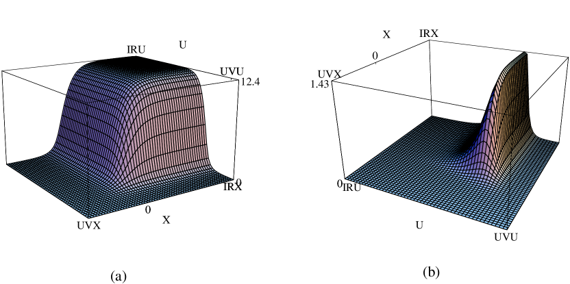
FIG. 1.: Solution of the SDE at $\mu/f_{\pi}=0.3$ for $N_{U}=70$, $N_{X}=60$: (a) real part; (b) imaginary part. Scale $\Lambda_{\rm qcd}$ is indicated by $0$ on $U$ and $X$ axes. Each number on the top of the vertical axis is the maximum value of $\mbox{Re}B/f_{\pi}$ or $\mbox{Im}B/f_{\pi}$.

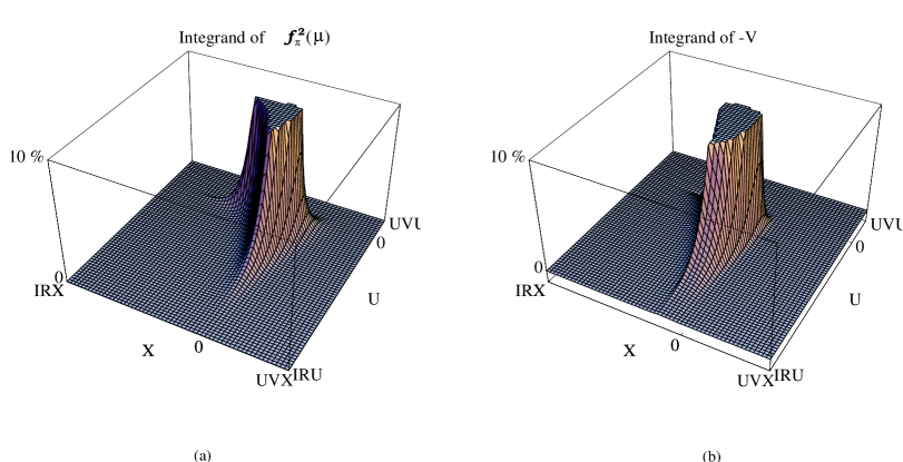
FIG. 2.: Integrands of (a) $f_{\pi}^{2}(\mu)$ and (b) $-\overline{V}[B_{\rm sol}]$ at $\mu/f_{\pi}=0.3$ for $N_{U}=70$, $N_{X}=60$. The upper 9/10 of each figure is clipped.

Figure 1(a) shows that the real part becomes small above $\Lambda_{\rm qcd}$. This behavior is similar to that of the solution at $T=\mu=0$. The dependence on $x$ of the imaginary part is similar to that of the real part. Since the imaginary part is an odd function in $u$, it becomes zero in the infrared region of $u$. Figure 2 shows that the dominant part of each integrand lies within the integration range. These imply that the choice of range in Eq. (54) is enough.

Next let us study the dependence of the results on the size of descretization. We show typical values of $f_{\pi}(\mu)/f_{\pi}$ in Fig. 3 and that of $\overline{V}[B_{\rm sol}]/f_{\pi}^{4}$ in Fig. 4 for four choices of the size of descretization, $(N_{U},N_{X})=(40,30)$, $(50,40)$, $(60,50)$ and $(70,60)$. This shows that the choice $(N_{U},N_{X})=(70,60)$ is large enough for the present purpose.

FIG. 3.: Typical values of $f_{\pi}(\mu)/f_{\pi}$ for four choices of the size of descretization, $(N_{U},N_{X})=(40,30)$, $(50,40)$, $(60,50)$ and $(70,60)$.

FIG. 4.: Typical values of $\overline{V}[B_{\rm sol}]/f_{\pi}^{4}$ for four choices of the size of descretization, $(N_{U},N_{X})=(40,30)$, $(50,40)$, $(60,50)$ and $(70,60)$.

Now we show the resultant values of $f_{\pi}(\mu)/f_{\pi}$ for two choices of initial trial functions in Fig. 5.

FIG. 5.: $\mu$-dependence of $f_{\pi}(\mu)/f_{\pi}$ at $T=0$ for two choices of the initial trial functions (A) and (B) in Eq. (58).

Below $\mu/f_{\pi}=3.0$ both the trial functions converge to the same non-trivial solution. The value of $f_{\pi}(\mu)$ increases slightly. The choice (B) in Eq. (58) converges to the trivial solution above $\mu/f_{\pi}=3.0$. However, the trial function (A) converges to a non-trivial solution, and the resultant value of $f_{\pi}(\mu)$ increases. Above $\mu/f_{\pi}=6.8$ (A) also converges to the trivial solution. In the range $3.0\leq\mu/f_{\pi}\leq 6.8$ two initial trial functions converge to different solutions: one corresponds to the chiral broken vacuum and another to the symmetric vacuum. Moreover, the trivial solution is always a solution of the SDE (22). Then we have to study which of the vacua is the true vacuum.

As we discussed in Sect. II, the true vacuum is determined by studying the effective potential. We show the value of the effective potential $\overline{V}[B_{\rm sol}]/f_{\pi}^{4}$ in Fig. 6.

FIG. 6.: $\mu$-dependence of the effective potential $\overline{V}[B_{\rm sol}]/f_{\pi}^{4}$ at $T=0$.

Since the value for the trivial solution is already subtracted from the expression in Eq. (26), positive (negative) value of $\overline{V}[B_{\rm sol}]$ implies that the energy of the chiral broken vacuum is larger (smaller) than that of the symmetric vacuum. For $3.0\leq\mu/f_{\pi}<5.23$, $\overline{V}[B_{\rm sol}]_{(A)}<\overline{V}[B_{\rm sol}]_{(B)}=0$, which implies that the chiral broken vacuum is energetically favored. On the other hand, for $5.23\leq\mu/f_{\pi}\leq 6.8$, $\overline{V}[B_{\rm sol}]_{(A)}>0$, and the chiral symmetric vacuum is the true vacuum. The chiral symmetry is restored at the point where the value of $\overline{V}[B_{\rm sol}]$ becomes positive: the chiral phase transition occurs at $\mu=460$ MeV ($\mu/f_{\pi}=5.23$). Since the value of the pion decay constant vanishes discontinuously at that point, the phase transition is clearly of first order. The non-trivial solutions for $5.23\leq\mu/f_{\pi}\leq 6.8$ correspond to meta-stable states, which were shown in Ref. [13] by assuming a momentum dependence of the mass function. The result here obtained by solving the SDE (22) agrees qualitatively with their result.

C $T\neq 0$ and $\mu=0$

At non-zero temperature we perform Matsubara frequency sum by truncating it at some finite number. Integration over the spatial momentum is done as shown in Eqs. (44) and (45). We have checked that the integration range given in the first line of Eq. (54) is large enough for the present purpose. Since the trial function (B) converges to the same solution as (A) for small $\mu$ in the case of $T=0$, it may be enough to use the trial function (A) for studying phase structure. Here and henceforth we use the trial function of type (A) only. First, we check dependences of the results on the truncation. In Fig. 7 we show the values of $f_{\pi}(T)/f_{\pi}$ at $T/f_{\pi}=0.5$, $1.0$ and $1.5$ for three choices of the truncation point: $N_{U}=10$, $15$ and $20$.

FIG. 7.: Values of $f_{\pi}(T)/f_{\pi}$ at $T/f_{\pi}=0.5$, $1.0$ and $1.5$ for three choices of the truncation point: $N_{U}=10$, $15$ and $20$.

It is clear that the choice $N_{U}=20$ is large enough as the truncation point for the present purpose.

Resultant temperature dependences of $f_{\pi}(T)/f_{\pi}$ and $\overline{V}[B_{\rm sol}]/f_{\pi}^{4}$ are shown in Fig. 8.

(a)

(b)

FIG. 8.: Temperature dependences of (a) $f_{\pi}(T)/f_{\pi}$ and (b) $\overline{V}[B_{\rm sol}]/f_{\pi}^{4}$.

The value of $f_{\pi}(T)$ does not change in low temperature region. It once increases around $T/f_{\pi}\sim 0.7$ and decreases to zero above that point, and finally reach to zero around $T/f_{\pi}=1.89$. Differently with the previous case the value of the potential reaches to zero around the temperature where the decay constant vanishes. Since there are numerical errors in the present analysis, we can not clearly show whether the decay constant and the potential vanish simultaneously. Our result shows that the chiral phase transition is of second order or of very weak first order, and that the critical temperature is around $T_{c}=166$ MeV.

D $T\neq 0$ and $\mu\neq 0$

Now, we solve the SDE when both $T$ and $\mu$ are non-zero. Infrared and ultraviolet cutoffs for $x$-integration are fixed as in the first equation of Eq. (54), and the sizes of descretizations are fixed to be $(N_{U},N_{X})=(20,60)$.

In the previous subsections we found that the phase transition at $T=0$ and $\mu\neq 0$ is of first order, while that at $T\neq 0$ and $\mu=0$ is of second order or of very weak first order. Then one can expect phase transitions of first order for small $T$ and large $\mu$, and those of weak first order for large $T$ and small $\mu$. First, we show the temperature dependence of $f_{\pi}(T)/f_{\pi}$ in Fig. 9 and that of $\overline{V}[B_{\rm sol}]/f_{\pi}^{4}$ in Fig. 10 for $\mu/f_{\pi}=1$, $2$, $3$, $4$ and $5$.

FIG. 9.: Temperature dependences of $f_{\pi L}/f_{\pi}$ for $\mu/f_{\pi}=1$, $2$, $3$, $4$ and $5$.

FIG. 10.: Temperature dependence of the effective potential $\overline{V}[B_{\rm sol}]/f_{\pi}^{4}$ for $\mu/f_{\pi}=1$, $2$, $3$, $4$ and $5$.

Figure 9 shows that in all the cases the values of the pion decay constant once increase around $T\sim f_{\pi}$ and decrease above that. These, especially for $\mu/f_{\pi}=1$ and $2$, behave as if the phase transitions are of second order. However, it is clear from Fig. 10 that the values of the effective potential $\overline{V}[B_{\rm sol}]$ become positive before the values of the pion decay constant vanish. Then the phase transitions are clearly of first order as in the case of $T=0$ and $\mu\neq 0$. To study phase transitions for smaller $\mu$ we concentrate on temperature dependences around phase transition points. Shown in Figs. 11 and 12 are temperature dependences of the pion decay constant and the effective potential for $\mu/f_{\pi}=0.25$, $0.5$ and $0.75$ together with those for $\mu/f_{\pi}=1$.

FIG. 11.: Temperature dependences of $f_{\pi}(T)/f_{\pi}$ for $\mu/f_{\pi}=0.25$, $0.5$, $0.75$ and $1.0$.

FIG. 12.: Temperature dependence of the effective potential $\overline{V}[B_{\rm sol}]/f_{\pi}^{4}$ for $\mu/f_{\pi}=0.25$, $0.5$, $0.75$ and $1.0$.

For $\mu/f_{\pi}=0.5$, $0.75$ and $1.0$ the values of the pion decay constant approach to zero as if the phase transitions are of second order. However, the values of the effective potential become positive before the values of the decay constant reaches to zero. Then we conclude that the phase transitions for $\mu/f_{\pi}=0.5$, $0.75$ and $1.0$ are clearly of first order. On the other hand, the phase transition for $\mu/f_{\pi}=0.25$ is of second order or of very weak first order.

FIG. 13.: Phase diagram obtained by the present analysis. Points indicated by $\diamond$ are the phase transition points of first order, and points by $+$ of second order or very weak first order.

Finally we show a phase diagram derived by the present analysis in Fig. 13. As was expected, phase transitions for small $T$ and large $\mu$ are of first order, and those for large $T$ and small $\mu$ are of second order or of very weak first order.

V Summary and Discussion

We analyzed the phase structure of QCD at finite temperature and density by solving the self-consistent Schwinger-Dyson equation for the quark propagator with the improved ladder approximation in the Landau gauge. A pion decay constant was calculated by using a generalized version of the Pagels-Stokar formula. Chiral phase transition point was determined by an effective potential for the propagator. When we raised the chemical potential $\mu$ with $T=0$, the value of the effective potential for the broken vacuum became bigger than that for the symmetric vacuum before the value of the pion decay constant vanished. The phase transition is clearly of first order. On the other hand, for $T\neq 0$ and $\mu=0$ the value of the effective potential for the broken vacuum reached to that for the symmetric vacuum around the temperature where the value of the pion decay constant vanished. The phase transition is of second order or very weak first order. We presented the resultant phase diagram on the general $T-\mu$ plane. Phase transitions are clearly of first order in most cases, and for small $\mu$ they are of second order or very weak first order. Our results show that it is important to use the effective potential to study the phase structure at finite temperature and density.

Finally, some comments are in order. Generally the running coupling should include the term from vacuum polarization of quarks and gluons at finite temperature and density. Moreover, the gluons at high temperature acquire an electric screening mass of order $gT$. [28] We dropped these effects, and used a running coupling and a gluon propagator of the same forms at $T=\mu=0$. (The same approximation was used in Ref. [17].) These effects can be included by using different running coupling and gluon propagator which depend explicitly on $T$ and $\mu$ such as in Refs. [13, 16].

The approximation of $A-1=C=0$ might not be good for high tempreture and/or density. However, inclusion of the deviations of $A-1$ and $C$ from zero requires the large number for truncating the Matsubara frequency, and it is not efficient to apply the method used in this paper. New method to solve the SDE may be needed. We expect that the inclusion of the deviations of $A-1$ and $C$ from zero does not change the structure of the phase transition shown in the present paper.

REFERENCES

- [1] R.D. Pisarski, BNL Report No. RP-941, hep-ph/9503330 (unpublished); G.E. Brown and M. Rho, Phys. Rep. 269, 333 (1996); T. Hatsuda, H. Shiomi and H. Kuwabara, Prog. Theor. Phys. 95, 1009 (1996).
- [2] T. Kugo, in Proceedings of 1991 Nagoya Spring School on Dynamical Symmetry Breaking, Nagoya, Japan, April 23–27, 1991, edited by K. Yamawaki (World Scientific Pub. Co., Singapore, 1991).
- [3] C. De Dominicis and P.C. Martin, J. Math. Phys. 5, 14 (1964); 5, 31 (1964).
- [4] J.M. Cornwall, R. Jackiw and E. Tomboulis, Phys. Rev. D 10, 2428 (1974).
- [5] For a review, see, e.g., R.W. Haymaker, Nuovo Cim. 14, 1 (1991); and references therein.
- [6] M. Bando, M. Harada and T. Kugo, Prog. Theor. Phys. 91, 927 (1994).
- [7] O.K. Kalashnikov, Pis’ma Zh. Kksp. Teor. Fiz. 41, 477 (1985) ( JETP Lett. 41 (1985)).
- [8] J. Cleymans, R.V. Gavai and E. Suhonen, Phys. Rep. 130, 217 (1986).
- [9] R. Gupta, G. Guralnik, G.W. Kilcup, A. Patel and S.R. Shape, Phys. Rev. Lett. 57, 2621 (1986).
- [10] T. Akiba, Phys. Rev. D 36, 1905 (1987).
- [11] O.K. Kalashnikov, Z. Phys. C39, 427 (1988).
- [12] A. Cabo, O.K. Kalashnikov and E.Kh. Veliev, Nucl. Phys. B299, 367 (1988).
- [13] A. Barducci, R. Casalbuoni, S. De Curtis, R. Gatto and G. Pettini, Phys. Rev. D 41, 1610 (1990).
- [14] A. Barducci, R. Casalbuoni, S. De Curtis, R. Gatto and G. Pettini, Phys. Lett. B 240, 429 (1990).
- [15] S.D. Odintsov and Yu.I. Shil’nov, Mod. Phys. Lett. A 6, 707 (1991).
- [16] K.-I. Kondo and K. Yoshida, Int. J. Mod. Phys. A 10, 199 (1995).
- [17] Y. Taniguchi and Y. Yoshida, Phys. Rev. D 55, 2283 (1997).
- [18] D.-S. Lee, C. N. Leung and Y. J. Ng, Phys. Rev. D 55, 6504 (1997); ibid 57, 5224 (1998).
- [19] H. Pagels and S. Stokar, Phys. Rev. D 20, 2947 (1979).
- [20] T. Matsubara, Prog. Theor. Phys. 14, 351 (1955).
- [21] T. Toimele, Int. J. Theor. Phys. 24, 901 (1985).
- [22] J. Kapusta, Finite-Temperature Field Theory (Cambridge University Press, Cambridge, 1989).
- [23] T. Kugo and M. Mitchard, Phys. Lett. B 282, 162 (1992); ibid 286, 355 (1992).
- [24] K.-I. Aoki, M. Bando, T. Kugo, M.G. Mitchard and H. Nakatani, Prog. of Theor. Phys. 84, 683 (1990).
- [25] R.D. Pisarski and M. Tytgat, Phys. Rev. D 54, R2989 (1996).
- [26] M. Tanabashi, in Proceedings of 1991 Nagoya Spring School on Dynamical Symmetry Breaking, Nagoya, Japan, April 23–27, 1991, edited by K. Yamawaki (World Scientific Pub. Co., Singapore, 1991).
- [27] J. Gasser and H. Leutwyler, Ann. Phys. (N.Y.) 158, 142 (1984).
- [28] K. Kajantie and J. Kapusta, Ann. of Phys. 160, 477 (1985).