DO-TH 98/12

DTP/98/36

July 1998

Photoproduction of Heavy Quarks

in Next-to-Leading Order QCD

with Longitudinally Polarized Initial States

I. Bojak

Institut für Physik, Universität Dortmund, D-44221 Dortmund, Germany

and

M. Stratmann

Department of Physics, University of Durham, Durham DH1 3LE, England

Abstract

We present all relevant details of our calculation of the complete next-to-leading order $({\cal{O}}(\alpha_{s}^{2}\alpha))$ QCD corrections to heavy flavor photoproduction with longitudinally polarized point-like photons and hadrons. In particular we provide analytical results for the virtual plus soft gluon cross section. We carefully address the relevance of remaining theoretical uncertainties by varying, for instance, the factorization and renormalization scales independently. Such studies are of importance for a meaningful first direct determination of the polarized gluon density $\Delta g$ from the total charm production spin asymmetry by the upcoming COMPASS experiment. It is shown that the scale uncertainty is considerably reduced in next-to-leading order, but the dependence on the charm quark mass is sizable at fixed target energies. Finally, we study several differential single-inclusive heavy quark distributions and, for the polarized HERA option, the total bottom spin asymmetry.

1 Introduction

Measuring the unpolarized gluon density of the nucleon $g(x,\mu^{2})$ at a scale $\mu$ as a function of the momentum fraction $x$ presents considerable theoretical and experimental challenges and thus serves as a benchmark for the steady progress in QCD. The determination of $g(x,\mu^{2})$ from measurements of the structure function $F_{2}$ in deep inelastic scattering (DIS) is hampered by the absence of direct couplings to the electroweak probes $(\gamma^{*},\,Z,\,W^{\pm})$. However, the increasingly precise $F_{2}$ data from HERA [1] still serve to constrain the small-$x$ behaviour of $g(x,\mu^{2})$ indirectly in the region $10^{-4}\lesssim x\lesssim 10^{-2}$ with an accuracy of about $10\%$ [2] from the observed scaling violations $\partial F_{2}(x,\mu^{2})/\partial\mu^{2}$. To determine $g(x,\mu^{2})$ over the entire $x$ region, i.e., also at larger values of $x$, studies of exclusive reactions like direct photon or di-jet production, where the gluon already enters in leading order (LO), are indispensable. Such measurements are often experimentally much more involved and less precise than inclusive DIS. Nevertheless, our knowledge of the unpolarized gluon density has greatly improved in the past few years (for recent QCD analyses see [3]), but in the region $x\gtrsim 0.1$ the situation is still far from being satisfactory. Here the uncertainty in $g(x,\mu^{2})$ easily amounts to about $100\%$ [4, 2, 3].

Concerning the spin properties of the gluons in a longitudinally polarized nucleon, the unpolarized gluon density $g(x,\mu^{2})$ is defined as the sum of the two possible helicity distributions, whereas the corresponding polarized gluon density $\Delta g(x,\mu^{2})$ is given by the difference. In general we have for a parton $f$ with $f=g,q,\overline{q}$

$${\mathrm{u}npolarized:}\quad f(x,\mu^{2}) =f_{+}(x,\mu^{2})+f_{-}(x,\mu^{2})\;\;,$$

$${\mathrm{p}olarized:}\quad \Delta f(x,\mu^{2}) =f_{+}(x,\mu^{2})-f_{-}(x,\mu^{2})\;\;.$$ (1)

Here $f_{+}$ and $f_{-}$ are the densities with the parton spin aligned and anti-aligned to the spin of the nucleon, respectively. In order to measure the two independent combinations in (1), we need experimental data and theoretical calculations distinguishing between different initial helicity states.

The long list of spin-dependent DIS experiments [5] and the recently completed next-to-leading order (NLO) framework for the evolution of the $\Delta f$ [6, 7] may lead to the expectation that the polarized gluon distribution $\Delta g(x,\mu^{2})$ should be known with almost similar accuracy as $g(x,\mu^{2})$ by now. This is, however, not the case as was revealed by all NLO analyses [8, 9, 10, 11] of presently available spin-dependent DIS data. In fact it turned out that the $x$-shape of $\Delta g$ is even almost completely unconstrained. This ignorance is, of course, also reflected in present values for the first moment of $\Delta g(x,\mu^{2})$, defined by

$$\Delta g(\mu^{2})\equiv\int_{0}^{1}dx\,\Delta g(x,\mu^{2})\;\;\;,$$ (2)

which can be estimated at best with an error of $100\%$ for the time being. $\Delta g(\mu^{2})$ plays an important rôle in our understanding of the spin-$1/2$ sum rule for nucleons

$$\frac{1}{2}=\frac{1}{2}\Delta\Sigma(\mu^{2})+\Delta g(\mu^{2})+L_{z}(\mu^{2})\;\;\;,$$ (3)

where $\Delta\Sigma$ is the total polarization carried by the quarks and antiquarks and $L_{z}$ denotes the sum of the non-perturbative angular momenta of all partons.

There are three main reasons for the present problems to pin down $\Delta g(x,\mu^{2})$:

• The measurements of the nucleon spin structure function $g_{1}$, the polarized analogue to the unpolarized structure function $F_{1}$, are still in a “pre-HERA” phase. The kinematical coverage of the fixed target experiments [5] is by far not sufficient to constrain $\Delta g(x,\mu^{2})$ from scaling violations $\partial g_{1}(x,\mu^{2})/\partial\mu^{2}$.

• As already mentioned, the unpolarized gluon density is also constrained by several exclusive reactions, but corresponding measurements in the polarized case are still missing.

• A momentum sum rule for spin-dependent parton densities is lacking, i.e., we cannot infer any constraint on $\Delta g$ from the already somewhat more precisely known polarized quark distributions. In addition, the spin-dependent parton densities $\Delta f$ defined in (1) are not required to be positive definite.

Nothing can be done about the last point, of course. The small-$x$ region of $g_{1}$ could be explored at HERA in case that the option to longitudinally polarize also the proton beam [12] will be realized in the future. First measurements of $\Delta g$ in exclusive reactions will be provided by the COMPASS fixed target experiment at CERN [13] and the BNL RHIC polarized $pp$ collider [14], which are both currently under construction.

For the determination of the gluon distribution, heavy quark ($Q=c,b$) photoproduction

$$\vec{\gamma}\vec{g}\rightarrow Q\bar{Q}$$ (4)

is an obvious choice (an arrow denotes a longitudinally polarized particle from now on). The reconstruction of an open heavy quark state is experimentally feasible, and in LO only the photon-gluon fusion (PGF) process in (4) contributes, which may lead to the hope that an unambiguous determination of $\Delta g$ can be performed. Thus open charm photoproduction will be used by the upcoming COMPASS experiment [13] to measure $\Delta g$. All theoretical studies of (4) have been performed only in LO so far [15, 16, 17, 13]. However, LO estimates usually suffer from a strong dependence on the a priori unknown factorization and renormalization scales. Also there are new NLO subprocesses induced by a light quark replacing the gluon in the initial state. Here the question arises if the PGF contribution (4) still dominates in the experimentally relevant kinematical region as is desirable for a precise determination of $\Delta g$. Finally, the NLO corrections have been shown to be sizable near threshold in the unpolarized case [18, 19]. Clearly, a NLO calculation also for the spin-dependent case is warranted in order to provide a meaningful interpretation of the forthcoming experimental results.

This paper provides all relevant details of the first calculation of the complete NLO $({\cal{O}}(\alpha_{s}^{2}\alpha))$ QCD corrections to heavy flavor photoproduction with point-like photons [20]. In [20] we only highlighted some of the most important phenomenological aspects, but we skipped most calculational details. In addition, we now present, again for the first time, NLO studies of differential single-inclusive heavy quark distributions. In the next section we will first make some general technical remarks concerning the polarized calculation. In Section 3 we recall the known LO results and extend them to $n$ dimensions as is required in course of the NLO calculation. In Section 4 we calculate the virtual one-loop corrections to (4) and examine the gluon bremsstrahlung process $\vec{\gamma}\vec{g}\rightarrow Q\bar{Q}g$ in detail. Section 5 is devoted to the new genuine NLO contribution with a light quark in the initial state $\vec{\gamma}\vec{q}\rightarrow Q\bar{Q}q$. The relevant formulae for calculating total and differential single-inclusive heavy quark cross sections can be found in Section 6, where we also present some further phenomenological studies. Finally, our main results are summarized in Section 7. In Appendix A we present the details of the phase space calculation. In particular, we focus on peculiarities which arise in a polarized calculation using dimensional regularization. Here we also supply the parametrizations of the parton momenta used in our calculations. Appendix B contains several helpful remarks concerning the calculation of the tensor integrals needed for the virtual corrections and Appendix C collects the analytical results for the polarized virtual plus soft cross section.

2 Some General Technical Remarks

In the calculation of the NLO corrections we will encounter the usual array of ultraviolet (UV), infrared (IR) and mass/collinear (M) singularities. We choose the framework of $n$-dimensional regularization to deal with all of these various types of singularities. Since our calculations proceed along similar lines as in [18] for the corresponding unpolarized case, we adopt their notation $n\equiv 4+\varepsilon$ for the deviation from four space-time dimensions in order to facilitate comparisons of the intermediate results. Of course, all results presented here can be easily converted to the more common choice $n\equiv 4-2\varepsilon$ by just replacing $\varepsilon\rightarrow-2\varepsilon$ accordingly. In the calculation we simply identify the dimension used to regularize the UV divergencies $n<4$ with the one used for the IR divergencies $n>4$. Thus we do not distinguish between $\varepsilon_{UV}<0$ and $\varepsilon_{IR}>0$, which for example leads to the following result for the basic loop integral:

$$\int\frac{d^{n}q}{q^{2\alpha}}=0\qquad{\mathrm{f}or}\quad\alpha>0\;\;.$$ (5)

Choosing the $n$-dimensional regularization method introduces some complications when polarized processes are investigated due to the unavoidable presence of $\gamma_{5}$ and the totally anti-symmetric Levi-Civita tensor $\epsilon_{\mu\nu\rho\sigma}$. First we shall recall how these quantities appear when projecting onto the helicity states of the incoming particles, and then we will explain how to deal with them in $n$ dimensions.

One can calculate the squared matrix elements for both unpolarized and polarized processes simultaneously using the squared matrix elements $\left|M\right|^{2}(h_{1},h_{2})$ for definite helicities $h_{1}$ and $h_{2}$ of the incoming particles:

$${\mathrm{u}npolarized:}\quad\overline{\left|M\right|}^{\>2} = \frac{1}{2}\left[\left|M\right|^{2}(++)+\left|M\right|^{2}(+-)\right]\;\;,$$ (6)

$${\mathrm{p}olarized:}\quad\Delta\left|M\right|^{2} = \frac{1}{2}\left[\left|M\right|^{2}(++)-\left|M\right|^{2}(+-)\right]\;\;.$$ (7)

This is of course highly desirable, since we obtain an important consistency check by comparing with the already known unpolarized results [18, 19]. To obtain $\left|M\right|(h_{1},h_{2})$ we use the standard helicity projection operators (see, e.g., [21])

$$\epsilon_{\mu}(k_{1},\lambda_{1})\,\epsilon^{*}_{\nu}(k_{1},\lambda_{1})=\frac{1}{2}\left[-g_{\mu\nu}+i\lambda_{1}\epsilon_{\mu\nu\rho\sigma}\frac{k_{1}^{\rho}k_{2}^{\sigma}}{k_{1}\cdot k_{2}}\right]$$ (8)

for incoming photons with momentum $k_{1}$ and helicity $\lambda_{1}$ (accordingly for gluons with $k_{2}$ and $\lambda_{2}$) and

$$u(k_{2},h)\bar{u}(k_{2},h)=\frac{1}{2}\not\!k_{2}(1-h\gamma_{5})$$ (9)

for incoming quarks with momentum $k_{2}$ and helicity $h$ (analogously for antiquarks).

We note that in the unpolarized case one has to average over the $n-2$ spin degrees of freedom for each incoming boson in $n$ dimensions. This can be achieved by the replacement $-1/2\,g_{\mu\nu}\rightarrow-1/(n-2)\,g_{\mu\nu}=-1/(2+\varepsilon)\,g_{\mu\nu}$ in (8) leaving (6) unchanged. However, it is convenient, both for the calculation and for the presentation of the results, to define instead

$$E_{\varepsilon}\equiv\left\{\begin{array}[]{cr}1/(1+\frac{\varepsilon}{2})&{\mathrm{u}npolarized}\\ 1&{\mathrm{p}olarized}\end{array}\right..$$ (10)

One can then perform the unpolarized and polarized calculations using (8), if one multiplies the results by a factor $E_{\varepsilon}$ for each incoming boson. We have also always identified the additional four-vector $\eta^{\sigma}$ usually appearing in (8) [21] to be that of the other incoming particle. This is possible since $k_{1}\cdot k_{2}=s/2\neq 0$ in (8) and simplifies the rather lengthy intermediate results considerably.

Figure 1: Graphical “rule” illustrating the replacement of the physical polarization sum $P_{\mu\nu}$ $(\circ)$ by $-g_{\mu\nu}$ $(\bullet)$ and appropriate ghost contributions (dashed lines). The minus signs in the lower half are due to the cut ghost loop.

As a further simplification one can drop all terms other than $-g_{\mu\nu}$ in the symmetric (unpolarized) part of (8). This of course means that unphysical polarizations will be kept in the polarization sums. However, unphysical photons decouple completely and unphysical gluons do not contribute as well, except for those subprocesses where one encounters a triple-gluon vertex. There one has to introduce incoming external ghost fields to cancel these unphysical parts [22], when using $-g_{\mu\nu}$ instead of the physical polarization sum $P_{\mu\nu}=\sum_{\lambda}\epsilon_{\mu}(\lambda)\epsilon^{*}_{\nu}(\lambda)$ [21]. Fig. 1 illustrates this elimination of such terms by adding appropriate external ghost contributions. The extra factors $(-1)$ multiplying each ghost contribution are due to the cut ghost loop.

The quantities $\epsilon_{\mu\nu\rho\sigma}$ and $\gamma_{5}$ introduced by (8) and (9), respectively, are of purely four-dimensional nature and there exists no straightforward continuation to $n\neq 4$ dimensions. We treat them by applying the HVBM prescription [23] which provides an internally consistent extension of $\epsilon_{\mu\nu\rho\sigma}$ and $\gamma_{5}$ to arbitrary dimensions. In this scheme the $\epsilon$-tensor continues to be a genuinely four-dimensional object and $\gamma_{5}$ is defined as in four dimensions, implying $\left\{\gamma^{\mu},\gamma_{5}\right\}=0$ for $\mu=0,\,1,\,2,\,3$ and $\left[\gamma^{\mu},\gamma_{5}\right]=0$ otherwise. This effectively splits the $n$-dimensional space into two subspaces, each one equipped with its own metric: one containing the four space-time dimensions and one containing the remaining $n-4$ dimensions, denoted “hat-space” henceforth. In the matrix elements we then encounter not only conventional $n$-dimensional scalar products of two momenta, like $k\cdot p=g_{\mu\nu}k^{\mu}p^{\nu}$, which can be expressed in terms of the usual Mandelstam variables, but also similar scalar products in the hat-space $\widehat{k\cdot p}=\hat{g}_{\mu\nu}\hat{k}^{\mu}\hat{p}^{\nu}$.

These additional terms would complicate the phase space calculations considerably, but one can eliminate most of them by choosing the coordinate system appropriately. The three-body phase space integration for the NLO $2\rightarrow 3$ processes exemplifies the problem: Since we are only interested in single-inclusive heavy quark cross sections in our calculation, it is possible to assign only the momenta of the two outgoing unobserved partons with non-vanishing hat-space contributions. The fully measured momenta of the initial states and of the observed heavy (anti)quark remain purely four-dimensional. A convenient choice of coordinates is the “Gottfried-Jackson frame” [24, 25], where the phase space integration is performed in the rest frame of these two unobserved particles. The remaining three momenta can then be oriented in such a way that they lie in, e.g., the $y-z$ plane. To further facilitate the phase space integrations one can finally choose one of these three vectors to have only a non-vanishing $z$-component (this freedom can be exploited to simplify the angular integrations). Using such a choice of coordinates, one thus ends up with only one scalar product of hat momenta $\hat{k}^{2}$, which simplifies the calculations considerably. In App. A one can find all required formulae concerning the phase space integration in the polarized case and the parametrizations of the parton momenta used in our calculations. For the additional integrals which depend on $\hat{k}^{2}$ we furthermore show in App. A that thanks to the heavy quark mass they are all at least of ${\cal O}(\varepsilon)$ and hence drop out when the limit $n\rightarrow 4$ is taken in the end. Thus we arrive at the welcome conclusion that in the particular case of our calculation hat momenta terms in the matrix elements do not contribute to the final result and can be ignored

. Concerning all $2\rightarrow 2$ subprocesses presented in Sections 3 to 5 it is then obvious that the same holds true. Since three of four external particles have their momentum fully measured, the fourth is determined by energy-momentum conservation and thus all hat components can be eliminated from the calculation.

3 Born Cross Section in $n$ Dimensions

Figure 2: Feynman diagrams for the LO photon-gluon fusion process $\gamma g\rightarrow Q\overline{Q}$.

In this section we will recall the well-known LO results for the unpolarized and polarized photoproduction of heavy flavors. Since we encounter $1/\varepsilon^{2}$ poles in our NLO calculation we have to extend these calculations up to ${\cal{O}}(\varepsilon^{2})$ in $n=4+\varepsilon$ dimensions. For the contributions to the Born amplitude depicted in Fig. 2 we use the following momentum assignment

$$\vec{\gamma}(k_{1})+\vec{g}(k_{2})\rightarrow Q(p_{1})+\overline{Q}(p_{2})$$ (11)

and the corresponding Mandelstam variables are given by

$$s=(k_{1}+k_{2})^{2},\quad t_{1}\equiv t-m^{2}=(k_{2}-p_{2})^{2}-m^{2},\quad u_{1}\equiv u-m^{2}=(k_{1}-p_{2})-m^{2}\;\;,$$ (12)

where $s+t_{1}+u_{1}=0$, $k_{1}^{2}=0$ (“on-shell” photon), $k_{2}^{2}=0$, and $p_{1}^{2}=p_{2}^{2}=m^{2}$ with $m$ denoting the heavy quark mass. All trace calculations in $n=4+\varepsilon$ dimensions are performed using the package TRACER [27]. In order to present the unpolarized and polarized results simultaneously in the most compact form, we will use $|\tilde{M}|^{2}$ here, and in the rest of the paper, to denote both the unpolarized $\overline{\left|M\right|}^{\>2}$ and polarized $\Delta\left|M\right|^{2}$ color-averaged squared matrix elements calculated according to Eqs. (6)-(10). Similarly, in (13) below $\tilde{B}_{QED}$ denotes either the unpolarized $B_{QED}$ or the polarized $\Delta B_{QED}$. The LO result can then be expressed as

$$|\tilde{M}|^{2}_{\mathrm{B}orn} = E_{\varepsilon}^{2}\,g_{s}^{2}e^{2}e_{Q}^{2}\tilde{B}_{QED}\;\;,$$

$$B_{QED} = \frac{t_{1}}{u_{1}}+\frac{u_{1}}{t_{1}}+\frac{4m^{2}s}{t_{1}u_{1}}\left(1-\frac{m^{2}s}{t_{1}u_{1}}\right)+\varepsilon\left(\frac{s^{2}}{t_{1}u_{1}}-1\right)+\varepsilon^{2}\frac{s^{2}}{4t_{1}u_{1}}\;\;,$$ (13)

$$\Delta B_{QED} = \left(\frac{t_{1}}{u_{1}}+\frac{u_{1}}{t_{1}}\right)\left(\frac{2m^{2}s}{t_{1}u_{1}}-1\right)\;\;,$$

where $g_{s}$ and $e$ are the strong and electromagnetic coupling constants, respectively, and $e_{Q}$ is the electromagnetic charge of the heavy quark in units of $e$, e.g., $e_{Q}=e_{c}=2/3$ for charm quarks. Notice that the polarized $\Delta B_{QED}$ retains its four-dimensional form and receives no ${\cal{O}}(\varepsilon)$ contributions in contrast to the unpolarized $B_{QED}$.

Using the standard $2\rightarrow 2$ phase space in $n$ dimensions,

$${\mathrm{dPS}}_{2}=\frac{2\pi}{s}\left[(4\pi)^{2+\varepsilon/2}\Gamma(1+\varepsilon/2)\right]^{-1}\left(\frac{t_{1}u_{1}-m^{2}s}{s}\right)^{\varepsilon/2}dt_{1}du_{1}$$ (14)

one can then write the $n$-dimensional Born cross section as

$$\frac{d^{2}\tilde{\sigma}^{(0)}_{g\gamma}}{dt_{1}du_{1}} = F_{\varepsilon}\delta(s+t_{1}+u_{1})|\tilde{M}|^{2},$$ (15)

$$F_{\varepsilon} \equiv \frac{\pi}{s^{2}}\left[(4\pi)^{2+\varepsilon/2}\Gamma(1+\varepsilon/2)\right]^{-1}\left(\frac{t_{1}u_{1}-m^{2}s}{\mu^{2}s}\right)^{\varepsilon/2},$$

where $F_{\varepsilon}$ collects all phase space factors given in (14), the flux factor $1/2s$, and the mass parameter $\mu$ introduced to keep the gauge couplings $g_{s}$ and $e$ dimensionless in $n$ dimensions. $\tilde{\sigma}$ denotes the unpolarized and polarized cross section $\sigma$ and $\Delta\sigma$, respectively. If one is only interested in the Born result itself, one can of course perform the $\varepsilon\rightarrow 0$ limit in (13) and simply use $F_{\varepsilon=0}=1/(16\pi s^{2})$. Our four-dimensional results for $\sigma^{(0)}_{g\gamma}$ and $\Delta\sigma^{(0)}_{g\gamma}$ (15) agree with those in [28, 18] and [29, 30], respectively.

4 NLO Gluon Contribution

Figure 3: The NLO virtual corrections to $\gamma g\rightarrow Q\overline{Q}$. Reversing the heavy quark lines, except for the non-planar graph (b), yields the remaining graphs. Massless particle loops similar to graph (i) vanish, see App. B.

Next we turn to the NLO corrections to the PGF process (4), where one-loop virtual and gluon bremsstrahlung contributions have to be taken into account. The one-loop virtual corrections displayed in Fig. 3 have the same $2\rightarrow 2$ kinematics as the Born graphs in Sec. 3 and can be also calculated using (11), (12), (14), and (15). At ${\cal{O}}(\alpha\alpha_{s}^{2})$ only the interference between the virtual $(V)$ and Born $(B)$ amplitudes of Figs. 2 and 3 contributes

$$|\tilde{M}|^{2}_{VB}=2{\mathrm{R}e}\left(\widetilde{M_{V}M_{B}^{*}}\right)=E_{\varepsilon}^{2}g_{s}^{4}e^{2}e_{Q}^{2}\left[2C_{F}\tilde{V}_{QED}+C_{A}\tilde{V}_{OK}\right],$$ (16)

where all quantities with a tilde denote again, as in Eq. (13), both the unpolarized and polarized expressions, e.g., $\tilde{V}_{QED}$ denotes either $V_{QED}$ or the spin-dependent $\Delta V_{QED}$. The color factors associated with the abelian and non-abelian parts are $C_{F}=(N_{C}^{2}-1)/(2N_{C})$ and $C_{A}=N_{C}$, respectively, where the number of colors is $N_{C}=3$ for QCD. We note that $\tilde{V}_{QED}$, which receives contributions only from the graphs (a), (c), (d) and (f)-(h) in Fig. 3, corresponds to the process where the gluon is replaced by a photon in the initial state, i.e., $\gamma\gamma\rightarrow Q\bar{Q}$. A complete NLO QCD ${\cal{O}}(\alpha^{2}\alpha_{s})$ calculation of this process has been performed recently in [30] for both the unpolarized and polarized case. Our NLO results for the QED-part of $\gamma g\rightarrow Q\bar{Q}$ agree analytically with the ones presented in [30].

In the loop-calculations we encounter Feynman integrals with up to four propagators in the denominator. We define the corresponding one-loop scalar one- ($A_{0}$), two- ($B_{0}$), three- ($C_{0}$) and four-point ($D_{0}$) functions as in Ref. [31], e.g., the four-point function needed for the box graphs in Figs. 3 (a), (b) is defined by

$$D_{0}(q_{1},q_{2},q_{3},m_{1},m_{2},m_{3},m_{4})\equiv$$

$$\!\!\!\!\mu^{-\varepsilon}\int\frac{d^{n}q}{(2\pi)^{n}}\frac{1}{(q^{2}-m_{1}^{2})[(q+q_{1})^{2}-m_{2}^{2}][(q+q_{1}+q_{2})^{2}-m_{3}^{2}][(q+q_{1}+q_{2}+q_{3})^{2}-m_{4}^{2}]}\;\;,$$

where the four external momenta satisfy $q_{1}+q_{2}+q_{3}+q_{4}=0$ and the $m_{i}$ are the internal masses. The required scalar integrals are conveniently collected in [31], however, we have checked them using the standard Feynman parametrization techniques. Each fermion propagator and each triple-gluon vertex in the loop introduces a loop momentum $q^{\mu}$ in the numerator. A glance at Fig. 3 then reveals that the maximal number of loop momenta we face in the numerator is one less than the number of propagators, except for graph (i). In particular, one has to deal with tensorial four-point integrals of first ($q^{\mu}$) to third ($q^{\mu}q^{\nu}q^{\rho}$) order and with tensorial three- and two-point integrals of first ($q^{\mu}$) and second ($q^{\mu}q^{\nu}$) order. We have developed a program which automatically reduces these tensor integrals to a set of scalar ones by using an adapted Passarino-Veltman decomposition method [32], which properly accounts for all possible $n$-dimensionally regulated divergencies in QCD. Since this procedure is quite common, we will just mention a few helpful details in App. B.

In the virtual cross section UV, IR and M singularities show up as $1/\varepsilon$ poles. In the non-abelian $OK$-part also double poles $1/\varepsilon^{2}$ occur when IR and M singularities coincide. The UV divergencies are removed by the renormalization procedure, which we implement using the common counterterm method (“renormalized perturbation theory”). The counterterms introduce additional contributions similar to those in Figs. 3 (c)-(i), but with the loops replaced by corresponding renormalization constant dependent “interactions”. For the internal gluon propagators we use the Feynman gauge. As the renormalization conditions we choose a modified $\overline{\mathrm{M}S}$ scheme, in which the heavy (anti-)quark is renormalized on-shell and the light quarks are renormalized using the standard $\overline{\mathrm{M}S}$ prescription. The heavy quark masses are defined as pole masses. The subtraction for the renormalization of the strong coupling constant explicitly removes the heavy quark loop contribution to the gluon self-energy shown in Fig. 3 (i), see also (B7) in App. B. This leads to a fixed flavor scheme with the produced heavy flavor on the one hand and $n_{lf}$ light flavors active in the running of $\alpha_{s}$ and in the parton evolution on the other hand [18, 33]. The renormalization constants needed for the construction of the counterterms are then calculated to be

$$Z_{m}-1 = \frac{g_{s}^{2}\mu^{-\varepsilon}}{16\pi^{2}}C_{F}3\left[\frac{2}{\hat{\varepsilon}_{m}}-\frac{4}{3}\right]\qquad({\mathrm{h}eavy~{}quark~{}mass}),$$

$$Z_{2}-1 = -\frac{g_{s}^{2}\mu^{-\varepsilon}}{16\pi^{2}}C_{F}\frac{2}{\hat{\varepsilon}_{m}}\qquad({\mathrm{h}eavy~{}quark~{}field}),$$

$$Z_{3}-1 = \frac{g_{s}^{2}\mu^{-\varepsilon}}{16\pi^{2}}\left[(2C_{A}-\beta_{0})\frac{2}{\hat{\varepsilon}}+\frac{2}{3}\frac{2}{\hat{\varepsilon}_{m}}\right]\qquad({\mathrm{g}luon~{}field}),$$ (18)

$$Z_{g}-1 = \frac{g_{s}^{2}\mu^{-\varepsilon}}{32\pi^{2}}\left[\beta_{0}\frac{2}{\hat{\varepsilon}}-\frac{2}{3}\frac{2}{\hat{\varepsilon}_{m}}\right]\qquad({\mathrm{c}oupling~{}constant}),$$

$$Z_{1F} = Z_{g}Z_{2}Z_{3}^{1/2}\qquad({\mathrm{q}uark~{}gluon~{}vertex}),$$

with the QCD beta function $\beta_{0}\equiv(11C_{A}-2n_{lf})/3$ for the $n_{lf}$ active light flavors, and we have used the definitions $2/\hat{\varepsilon}\equiv 2/\varepsilon+\gamma_{E}-\ln(4\pi)$ and $2/\hat{\varepsilon}_{m}\equiv 2m^{\varepsilon}/\hat{\varepsilon}$ with the Euler constant $\gamma_{E}$. $Z_{1F}$ is determined to ${\cal O}(g_{s}^{2})$ using the shown Slavnov-Taylor identity, and the quark photon vertex renormalization constant can be obtained from $Z_{1F}$ by either setting $C_{A}=0$ or by using the QED Ward-Takahashi identity $Z_{1F}^{QED}=Z_{2}$ [34]. The coupling constant $g_{s}$ in (4) and in the matrix element calculations is the renormalized one in the counterterm method. We then of course use the renormalization group (RG) improved running coupling $g_{s}(\mu_{r}^{2})$ in the calculation, where $\mu_{r}$ is the renormalization scale at which the subtractions are performed. We have checked that the procedure outlined above is completely equivalent to the one used in [18] in the corresponding unpolarized calculation. In [18] the renormalization is performed by replacing the bare mass and strong coupling constant in the Born cross section with the corresponding renormalized quantities (see [18] for more details). Their relation between the bare and the renormalized mass can be obtained by expanding $m_{\mathrm{b}are}=Z_{m}m$ in $\varepsilon$ using the $Z_{m}$ in (4). Analogously, the series in $\varepsilon$ of $g_{s}^{\mathrm{b}are}=Z_{g}g_{s}$ using the $Z_{g}$ of (4) in combination with the RG running leads to their relation for the strong coupling

$$g_{s}^{\mathrm{b}are}\rightarrow g_{s}(\mu_{r}^{2})\left[1+\frac{g_{s}^{2}(\mu_{r}^{2})}{32\pi^{2}}\left\{\left(\frac{2}{\hat{\varepsilon}}+\ln\frac{\mu_{r}^{2}}{\mu^{2}}\right)\beta_{0}^{f}-\frac{2}{3}\ln\frac{m^{2}}{\mu_{r}^{2}}\right\}\right]\;\;,$$ (19)

where $\beta_{0}^{f}$ is defined as $\beta_{0}$ above, but with $n_{f}=n_{lf}+1$ instead of $n_{lf}$ flavors. The first term in the curly brackets corresponds to the usual $\overline{\mathrm{MS}}$ prescription and the second one removes the heavy quark contribution to the gluon self-energy, as already mentioned.

Figure 4: Feynman diagrams for the NLO gluon bremsstrahlung process $\gamma g\rightarrow Q\overline{Q}g$. Reversing the heavy quark lines yields the remaining graphs. In the unpolarized calculation the ghost contributions (e) and (f) have to be subtracted to cancel unphysical polarization contributions, see the discussion concerning Fig. 1.

The IR singularities of the virtual cross section are canceled by the soft part of the gluon bremsstrahlung contributions. The corresponding Feynman diagrams are shown in Fig. 4 and the momenta assignment is

$$\vec{\gamma}(k_{1})+\vec{g}(k_{2})\rightarrow Q(p_{1})+\overline{Q}(p_{2})+g(k_{3})\;\;.$$ (20)

In the calculation of this process we keep the kinematical invariants as defined in (12) and introduce seven additional ones [18]:

$$\begin{array}[]{lll}s_{3}=(k_{3}+p_{2})^{2}-m^{2}\;\;,&s_{4}=(k_{3}+p_{1})^{2}-m^{2}\;\;,&s_{5}=(p_{1}+p_{2})^{2}=-u_{5}\;\;,\\ t^{\prime}=(k_{2}-k_{3})^{2}\;\;,&u^{\prime}=(k_{1}-k_{3})^{2}\;\;,&\\ u_{6}=(k_{2}-p_{1})^{2}-m^{2}\;\;,&u_{7}=(k_{1}-p_{1})^{2}-m^{2}\;\;.&\end{array}$$ (21)

Of course, only five of these invariants are independent for a $2\rightarrow 3$ process and hence there are many useful relations among the quantities in (12) and (21), like

$$\begin{array}[]{lll}u^{\prime}=-s-u_{1}-u_{7}\;\;,&t^{\prime}=-s-t_{1}-u_{6}\;\;,&u_{5}=t_{1}+u_{1}+s_{3}\;\;,\\ s_{3}=s+u_{6}+u_{7}\;\;,&s_{4}=s+t_{1}+u_{1}\;\;.&\end{array}$$ (22)

The real gluon bremsstrahlung cross section $(R)$ can then be written as

$$\left(\frac{d^{2}\tilde{\sigma}^{(1)}_{g\gamma}}{dt_{1}du_{1}}\right)^{R} = F_{\varepsilon}G_{\varepsilon}\int d\Omega_{\varepsilon}|\tilde{M}_{R}|^{2}\;\;,$$ (23)

$$G_{\varepsilon} \equiv \frac{\mu^{-\varepsilon}}{2\pi(4\pi)^{2+\varepsilon/2}}\frac{\Gamma(1+\varepsilon/2)}{\Gamma(1+\varepsilon)}\frac{s_{4}^{1+\varepsilon}}{(s_{4}+m^{2})^{1+\varepsilon/2}}\;\;,$$

$$\int d\Omega_{\varepsilon} \equiv \int_{0}^{\pi}d\theta_{1}\sin^{1+\varepsilon}\theta_{1}\int_{0}^{\pi}\sin^{\varepsilon}\theta_{2}\;\;,$$

where we have used the standard $2\rightarrow 3$ phase space (see App. A). For simplicity we have already replaced the phase space integration over the $(n-4)$-dimensional hat-space by “1” in (23), since the hat parts do not give any contribution to the final result as discussed in Sec. 2 and App. A. Hence all hat terms in the squared matrix element $|\tilde{M}_{R}|^{2}$ below have to be dropped before $|\tilde{M}_{R}|^{2}$ is inserted into (23). $G_{\varepsilon}$ parametrizes the differences between the $2\rightarrow 2$ prefactor $F_{\varepsilon}$ defined in (15) and the $2\rightarrow 3$ prefactor, which is convenient for further considerations. The squared matrix element can again be split into an abelian and a non-abelian part

$$|\tilde{M}_{R}|^{2}=\widetilde{M_{R}M_{R}^{*}}=E_{\varepsilon}^{2}g_{s}^{4}e^{2}e_{Q}^{2}\left[2C_{F}\tilde{R}_{QED}+C_{A}\tilde{R}_{OK}\right]\;\;.$$ (24)

Concerning the angular integration $\int d\Omega_{\varepsilon}$ in (23) we note that the Mandelstam variables of (12) and (21) are of three distinct types: Using the “set I” parametrization of the parton momenta in terms of the angles $\theta_{1}$ and $\theta_{2}$ in App. A, the Mandelstam variables $t^{\prime}$ and $u_{6}$ are of the $[ab]$-type $a+b\cos\theta_{1}$, whereas $s_{3}$, $s_{5}$, $u^{\prime}$ and $u_{7}$ are of the $[ABC]$-type $A+B\cos\theta_{1}+C\sin\theta_{1}\cos\theta_{2}$. Here $a$, $b$, $A$, $B$, and $C$ are functions of the angular-independent ($[\cdot]$-type) Mandelstam variables $s$, $t_{1}$, $u_{1}$, $s_{4}$ and of the heavy quark mass $m$. Extensive partial fractioning using the relations given in (22) reduces all phase space integrals to the standard form

$$I_{\varepsilon}^{(k,l)}=\int d\Omega_{\varepsilon}(a+b\cos\theta_{1})^{-k}(A+B\cos\theta_{1}+C\sin\theta_{1}\cos\theta_{2})^{-l}\;\;,$$ (25)

which can be performed analytically. This reduction procedure can be completely automatized using a general set of transformation rules based on relations like in (22), that is $[ABC]=[\cdot]+[ab]+[ABC]$. As an example we demonstrate here two reduction steps for $1/(s_{3}u_{6}u_{7})$ using $s_{3}=s+u_{6}+u_{7}$:

$$\frac{1}{s_{3}u_{6}u_{7}}=\frac{1}{s}\left(\frac{1}{u_{6}u_{7}}-\frac{1}{u_{6}s_{3}}-\frac{1}{s_{3}u_{7}}\right)\qquad{\mathrm{and}}\qquad\frac{1}{s_{3}u_{7}}=\frac{1}{u_{6}^{\prime}u_{7}}-\frac{1}{u_{6}^{\prime}s_{3}}\;\;,$$ (26)

with $u_{6}^{\prime}\equiv s+u_{6}$. In this way $1/(s_{3}u_{6}u_{7})$ can be completely reduced to the $[ab][ABC]$ form required in (25), but the auxiliary $[ab]$ variable $u_{6}^{\prime}$ has to be introduced in our example. This always happens for two $[ABC]$ variables in the denominator. Though the integrals with this kind of auxiliary variables are as straightforward as the others, they can also be easily avoided by introducing a different parametrization for the parton momenta (“set II” in App. A). In this particular set, $u^{\prime}$ and $u_{7}$ are of the $[ab]$-type instead of $t^{\prime}$ and $u_{6}$ for “set I”. So in our example above, $1/(s_{3}u_{7})$ would be already of the $[ab][ABC]$ type using “set II” and no further reduction would be necessary. As a check for the correctness of our phase space calculations, we have proceeded in both ways. It should be remarked that a third conceivable parametrization of the momenta is not required in our calculations.

The needed integrals $I^{(k,l)}$ are conveniently collected in [31]. We have recalculated them and also the few additional ones that occur in the reduction method using solely “set I”. The integrals are straightforward to calculate by using two “tricks”: Firstly, most integrals can be derived from a basic one by partial differentiation with respect to the parameters $a$ and $A$ in (25). Note that one has to be careful in case of “collinear” parameters $a^{2}=b^{2}$ or $A^{2}=B^{2}+C^{2}$, though. Secondly, the transformation

$$I_{\varepsilon}^{(k,l)}=I_{\varepsilon}^{(l,k)}(a\leftrightarrow A,b\rightarrow-\sqrt{B^{2}+C^{2}},B\rightarrow\frac{-bB}{\sqrt{B^{2}+C^{2}}},C\rightarrow\frac{-bC}{\sqrt{B^{2}+C^{2}}})$$ (27)

is often helpful. In particular one can transform “$A^{2}=B^{2}+C^{2}$” collinearities into “$a^{2}=b^{2}$” ones in this way [35]. One can also prove $I_{\varepsilon}^{(k,l)}(u_{6},u_{7})=I_{\varepsilon}^{(l,k)}(u_{6},u_{7},t_{1}\leftrightarrow u_{1})$ using this transformation.

In order to isolate the divergencies appearing in the soft $s_{4}\rightarrow 0$ limit, which cancel the IR singularities of the virtual cross section, we examine the bremsstrahlung result in two regions: that for hard ($s_{4}>\Delta$) and that for soft ($s_{4}<\Delta$) gluons [18]. Here the auxiliary quantity $\Delta$ is chosen small enough to be negligible in comparison to $s$, $t_{1}$, $u_{1}$ and $m^{2}$. In the hard ($H$) region $\Delta$ effectively cuts off the IR singularities, so that only the M singularities remain. Thus no double poles will be encountered and one needs $G_{\varepsilon}$ in (23) only to ${\cal O}(\varepsilon)$:

$$G_{\varepsilon}^{H}\equiv\frac{2(4\pi)^{4}(s_{4}+m^{2})}{s_{4}}G_{\varepsilon}\simeq 16\pi\left[1+\frac{\varepsilon}{2}\left(\gamma_{E}-\ln(4\pi)+\ln\frac{s_{4}^{2}}{\mu^{2}(s_{4}+m^{2})}\right)\right]\;\;,$$ (28)

where we have also absorbed some additional factors into $G_{\varepsilon}^{H}$ for convenience. The hard gluon cross section then becomes

$$\left(\frac{d^{2}\tilde{\sigma}^{(1)}_{g\gamma,OK}}{dt_{1}du_{1}}\right)^{H} = C_{A}F_{\varepsilon}G_{\varepsilon}^{H}E_{\varepsilon}^{2}\alpha_{s}^{2}\alpha e_{Q}^{2}\frac{2}{\varepsilon}\tilde{H}_{OK,{\mathrm{p}ole}}+{\cal O}(1)\;\;,$$

$$H_{OK,{\mathrm{p}ole}} = \frac{(\rho-1+1/\rho)^{2}}{s_{4}}\left[\frac{t_{1}}{u_{1}}\frac{1}{\rho}+\frac{u_{1}}{t_{1}}\rho+\frac{4m^{2}s}{t_{1}u_{1}}\left(1-\frac{m^{2}s}{t_{1}u_{1}}\right)\right]\;\;,$$ (29)

$$\Delta H_{OK,{\mathrm{p}ole}} = \frac{2\rho-3+2/\rho}{s_{4}}\left(\frac{t_{1}}{u_{1}}\frac{1}{\rho}+\frac{u_{1}}{t_{1}}\rho\right)\left(\frac{2m^{2}s}{t_{1}u_{1}}-1\right)\;\;,$$

where only the collinear pole contribution of the non-abelian $OK$ part is shown. The hard abelian $QED$ part is completely finite. The parameter $\rho\equiv 1-s_{4}/u_{1}$ becomes one in the soft limit $s_{4}\rightarrow 0$, and one can clearly see the approach to an IR singularity proportional to the Born $\tilde{B}_{QED}$ of (13). The finite contributions are too long to be presented here in an analytical form, but they can be found in our computer program, which is available upon request. Our unpolarized results agree with those of [18].

Turning now to the soft gluon region, we find that one can write the Mandelstam variables in (21) in the soft limit $s_{4}\rightarrow 0$ as

$$\begin{array}[]{lll}s_{3}=s_{4}\underline{s_{3}}\;\;,&t^{\prime}=s_{4}\underline{t^{\prime}}\;\;,&u^{\prime}=s_{4}\underline{u^{\prime}}\;\;,\\ u_{5}=-s+s_{4}\underline{u_{5}}\;\;,&u_{6}=u_{1}+s_{4}\underline{u_{6}}\;\;,&u_{7}=t_{1}+s_{4}\underline{u_{7}}\;\;,\end{array}$$ (30)

where the underlined quantities are finite dimensionless functions of the $2\rightarrow 2$ Mandelstam variables (12) and $m^{2}$. In terms of these variables one can easily single out the IR singularities by collecting different powers in $s_{4}$. Applying the $s_{4}\rightarrow 0$ limit on the factor $G_{\varepsilon}$ in (23), one obtains a $s_{4}^{1+\varepsilon}$ dependence. Thus one only has to keep track of those parts of the squared matrix element exhibiting a $1/s_{4}^{2}$ pole in the soft limit, since all other terms vanish for $s_{4}\rightarrow 0$. In this way one can easily derive the soft limit of $\tilde{R}_{QED}$ and $\tilde{R}_{OK}$ in (24)

$$\tilde{S}_{QED} = -\frac{2}{s_{4}^{2}}\left[m^{2}\left(1+\frac{1}{\underline{s_{3}^{2}}}\right)+\frac{(2m^{2}-s)}{\underline{s_{3}}}\right]\tilde{B}_{QED},$$

$$\tilde{S}_{OK} = \frac{2}{s_{4}^{2}}\left[\frac{1}{\underline{t^{\prime}}}\left(\frac{t_{1}}{\underline{s_{3}}}+u_{1}\right)+\frac{(2m^{2}-s)}{\underline{s_{3}}}\right]\tilde{B}_{QED},$$ (31)

using the polarized and unpolarized $B_{QED}$ and $\Delta B_{QED}$ in (13), respectively, in agreement with [18].

We rewrite the IR-divergent $s_{4}^{-1+\varepsilon}$-dependence in terms of the $\Delta$-distribution:

$$\int_{0}^{\Delta}ds_{4}\,f(s_{4})[g(s_{4})]_{\Delta}\equiv\int_{0}^{\Delta}ds_{4}\,\left[f(s_{4})-f(0)\right]g(s_{4})\;\;,$$ (32)

where $[g(s_{4})]_{\Delta}$ is singular and $f(s_{4})$ is finite for $s_{4}\rightarrow 0$. In particular we need the following identity

$$s_{4}^{-1+\varepsilon}=\frac{\Delta^{\varepsilon}}{\varepsilon}\delta(s_{4})+[s_{4}^{-1+\varepsilon}]_{\Delta}\;\;.$$ (33)

This yields for the $s_{4}$-integration of a function ${\cal H}(s_{4})$ with a soft pole $s_{4}^{-1+\varepsilon}{\cal S}(s_{4})$ and a finite ${\cal F}(s_{4})$ part:

$$\int_{0}^{s_{4}^{\mathrm{m}ax}}ds_{4}{\cal H}(s_{4})\equiv\int_{0}^{s_{4}^{\mathrm{m}ax}}ds_{4}\left[s_{4}^{-1+\varepsilon}{\cal S}(s_{4})+{\cal F}(s_{4})\right]$$ (34)

$$= \int_{0}^{\Delta}ds_{4}\left[\frac{\Delta^{\varepsilon}}{\varepsilon}\delta(s_{4}){\cal S}(s_{4})+\{{\cal S}(s_{4})-{\cal S}(0)\}s_{4}^{-1+\varepsilon}+{\cal F}(s_{4})\right]+\int_{\Delta}^{s_{4}^{\mathrm{m}ax}}ds_{4}{\cal H}(s_{4})$$

$$\simeq \int_{0}^{s_{4}^{\mathrm{m}ax}}ds_{4}\left[\frac{\Delta^{\varepsilon}}{\varepsilon}\delta(s_{4}){\cal S}(s_{4})+\Theta(s_{4}-\Delta){\cal H}(s_{4})\right]$$

where $\Theta$ is the Heavyside step function. In the last step we have explicitly used that $\Delta$ is small enough to be negligible with respect to the $2\rightarrow 2$ Mandelstam variables (12) and $m^{2}$, taking ${\cal S}(\Delta)\simeq{\cal S}(0)\neq 0$ and ${\cal F}(\Delta)\simeq{\cal F}(0)=0$ as the finite limits.

We can thus write the total gluon bremsstrahlung result by multiplying the hard cross section (4) with $\Theta(s_{4}-\Delta)$ and adding the soft cross section obtained from (4) with the $s_{4}^{-1+\varepsilon}$ replaced by $\delta(s_{4})\Delta^{\varepsilon}/\varepsilon$ according to (34). Using this replacement and performing the angular integrations $d\Omega_{\varepsilon}$ the soft $(S)$ gluon cross section is then given by

$$\left(\frac{d^{2}\tilde{\sigma}^{(1)}_{g\gamma,OK}}{dt_{1}du_{1}}\right)^{S} = C_{A}F_{\varepsilon}G_{\varepsilon}^{S}E_{\varepsilon}^{2}\alpha_{s}^{2}\alpha e_{Q}^{2}\frac{\tilde{B}_{QED}}{2}\Bigg{[}\frac{4}{\varepsilon^{2}}+\frac{2}{\varepsilon}\ln\frac{t_{1}}{u_{1}}+\ln\varkappa\ln\frac{u_{1}}{t_{1}}+\frac{1}{2}\ln^{2}\frac{u_{1}}{t_{1}}+{}$$

$${}-\frac{1}{2}\ln^{2}\varkappa+{\mathrm{L}i}_{2}\left(1-\frac{t_{1}}{\varkappa u_{1}}\right)-{\mathrm{L}i}_{2}\left(1-\frac{u_{1}}{\varkappa t_{1}}\right)+\frac{2m^{2}-s}{s\beta}S(\varkappa)\Bigg{]}\;\;,$$

$$\left(\frac{d^{2}\tilde{\sigma}^{(1)}_{g\gamma,QED}}{dt_{1}du_{1}}\right)^{S} = 2C_{F}F_{\varepsilon}G_{\varepsilon}^{S}E_{\varepsilon}^{2}\alpha_{s}^{2}\alpha e_{Q}^{2}\frac{\tilde{B}_{QED}}{2}\left[-\frac{2}{\varepsilon}+1+\frac{2m^{2}-s}{s\beta}(1-S(\varkappa))\right],$$ (35)

with

$$S(\varkappa) \equiv -\frac{2}{\varepsilon}\ln\varkappa+{\mathrm{L}i}_{2}\left(\varkappa^{2}\right)-\ln^{2}\varkappa+2\ln\varkappa\ln(1-\varkappa^{2})-\zeta(2)\;\;,$$

$$G_{\varepsilon}^{S} \equiv \frac{2(4\pi)^{4}m^{2}\varepsilon}{s_{4}^{2}}G_{\varepsilon}\rightarrow 16\pi e^{\varepsilon(\gamma_{E}-\ln(4\pi))/2}\left(1-\frac{3}{8}\zeta(2)\varepsilon^{2}\right)\left(\frac{\Delta^{2}}{\mu^{2}m^{2}}\right)^{\varepsilon/2}\delta(s_{4}),$$ (36)

and where we have used $\beta\equiv\sqrt{1-4m^{2}/s}$, $\varkappa\equiv(1-\beta)/(1+\beta)$, the dilogarithm function ${\mathrm{L}i}_{2}$ as defined in [36], and the Riemann zeta function $\zeta(2)=\pi^{2}/6$. Adding the soft cross section (4) to the renormalized virtual cross section obtained from (16) and (4) removes all IR singularities in the latter, including the $1/\varepsilon^{2}$ poles. An additional $1/\varepsilon$ pole in the $OK$ part of (4) will be eventually canceled upon adding the soft $\delta(1-x)$ contribution of the mass factorization cross section (4) discussed below. Our unpolarized results are again identical to those of [18]. In addition we have checked that the abelian $QED$ part of the polarized (and unpolarized) result is in complete analytical agreement with the NLO expressions for $\gamma\gamma\rightarrow Q\bar{Q}$ presented in [30].

To obtain the final result for the gluon cross section, the remaining M singularities in the hard gluon cross section have to be removed as well. This can be achieved by the standard mass factorization procedure. To ${\cal O}(\alpha_{s}^{2}\alpha)$ the reduced finite gluon cross section is given by [18]

$$\frac{d^{2}\tilde{\sigma}^{(1)}_{g\gamma}}{dt_{1}du_{1}}(\mu_{f}^{2})=\frac{d^{2}\tilde{\sigma}^{(1)}_{g\gamma}}{dt_{1}du_{1}}(\mu^{2})-{}$$

$${}-\frac{\alpha_{s}}{2\pi}\int_{0}^{1}dx\left[\tilde{P}_{gg}(x)\frac{2}{\varepsilon}+\tilde{F}_{gg}(x,\mu_{f}^{2},\mu^{2})\right]x\left[\frac{d^{2}\tilde{\sigma}^{(0)}_{g\gamma}}{dt_{1}du_{1}}\right]{s\rightarrow xs\choose t_{1}\rightarrow xt_{1}}\;\;,$$

where $\mu_{f}$ denotes the factorization scale at which the subtraction is performed, and $\tilde{F}$ represents the usual freedom in choosing a factorization prescription. In the $\overline{\mathrm{M}S}$ scheme, which we use, $\tilde{F}$ is given by

$$\tilde{F}_{ij}(x,\mu_{f}^{2},\mu^{2})=\tilde{P}_{ij}(x)\left(\gamma_{E}-\ln(4\pi)+\ln\frac{\mu_{f}^{2}}{\mu^{2}}\right)\;\;.$$ (38)

The $\tilde{P}_{ij}$ in (4) and (38) are the usual unpolarized ($P_{ij}$) and polarized ($\Delta P_{ij}$) LO Altarelli-Parisi splitting functions [37]

$$P_{gg}(x) = \Theta(1-x-\delta)2C_{A}\left(\frac{1}{1-x}+\frac{1}{x}-2+x(1-x)\right)+P_{gg}^{\delta}(x)\;\;,$$

$$\Delta P_{gg}(x) = \Theta(1-x-\delta)2C_{A}\left(\frac{1}{1-x}-2x+1\right)+P_{gg}^{\delta}(x)\;\;,$$ (39)

$$P_{gg}^{\delta}(x) = \delta(1-x)\left(\frac{\beta_{0}}{2}+2C_{A}\ln\delta\right)\;\;.$$

Since we have regularized all soft singularities in our calculation by a small parameter $\Delta$ as outlined above, we have to stick to the same framework here to deal with the soft $x\rightarrow 1$ divergency of $\tilde{P}_{gg}$ consistently and cannot simply use the usual $+$–prescription $1/(1-x)_{+}$. In (4) we have thus introduced another small auxiliary quantity $\delta$ [18, 38]. Of course, $\Delta$ introduced above and $\delta$ are not independent, since they are related via the mass factorization by $\delta=\Delta/(s+t_{1})$. $\beta_{0}$ in (4) includes only the $n_{lf}$ light flavors as in (4).

Inserting (4) in (4) one gets schematically

$$\int_{0}^{1}dx[\delta(1-x)A+\Theta(1-x-\delta)B(x)]x\delta(x(s+t_{1})+u_{1})C(xs,xt_{1},u_{1})$$

$$= \delta(s_{4})AC(s,t_{1},u_{1})+\Theta(s_{4}-\Delta)\left[-u_{1}B\left(\frac{-u_{1}}{s+t_{1}}\right)C\left(\frac{-u_{1}s}{s+t_{1}},\frac{-u_{1}t_{1}}{s+t_{1}},u_{1}\right)\right]\;\;,$$

where we have explicitly used the relation between $\delta$ and $\Delta$. Thus the contribution from mass factorization naturally splits into a soft and a hard part, which can be added to the corresponding cross sections. As already mentioned, the $2/\varepsilon$ pole in the soft $\delta(1-x)$ part of (4) cancels the remaining pole in the $OK$ part of the soft cross section (4). In the hard cross section (4) the $2/\varepsilon$ collinear pole is removed and one is left over with the finite contributions from the pole part obtained from the $\varepsilon$-expansion of the prefactor. Examining this factor (28) and our choice for the $\overline{\mathrm{MS}}$ factorization scheme in (38), it is easy to see that the reduced hard gluon cross section can be simply obtained from (4) by setting

$$F_{\varepsilon}\tilde{G}_{\varepsilon}^{H}\rightarrow\frac{1}{s^{2}}\;\;,\qquad E_{\varepsilon}\rightarrow 1\;\;,\qquad{\mathrm{a}nd}\qquad\frac{2}{\varepsilon}\rightarrow\ln\frac{s_{4}^{2}}{m^{2}(s_{4}+m^{2})}-\ln\frac{\mu_{f}^{2}}{m^{2}}\;\;,$$ (41)

where one can now perform the $\varepsilon\rightarrow 0$ limit. Again we agree with the unpolarized reduced hard gluon cross section of [18].

To complete the calculation of the gluon cross section, we now add the $\delta(s_{4})$ mass factorization contribution in (4), see Eq. (4), to the renormalized virtual plus soft part $(V+S)$. We write the result in three parts using the usual abelian and non-abelian split and, in addition, separating off the part proportional to $\beta_{0}/2$. The latter piece vanishes if one identifies the renormalization scale with the factorization scale, i.e., $\mu_{r}=\mu_{f}$, as is usually done:

$$\left(\frac{d^{2}\hat{\sigma}^{(1)}_{g\gamma}}{dt_{1}du_{1}}\right)^{\mathrm{V}+S}=\frac{\alpha_{s}^{2}\alpha e_{Q}^{2}}{s^{2}}\left[2C_{F}\left(\tilde{L}_{QED}+\tilde{L}_{QED}^{\Delta}\right)+C_{A}\left(\tilde{L}_{OK}+\tilde{L}_{OK}^{\Delta}\right)+\frac{\beta_{0}}{2}\tilde{L}_{RF}\right]\;\;.$$ (42)

The $\tilde{L}^{\Delta}$ explicitly depend on the auxiliary quantity $\Delta$. The polarized $\Delta L$ are presented in App. C and the unpolarized $L$ are in complete agreement with those obtainable from App. A of [18] and App. D of [31]. The numerical treatment of the $\tilde{L}^{\Delta}$ terms is discussed in App. C.

To conclude this section we note that the presented results have been calculated for a detected heavy antiquark in the final state, because the heavy quark was integrated out in the calculations. But since all gluon matrix elements are symmetric with respect to $p_{1}\leftrightarrow p_{2}$, the same gluon cross section holds for a detected heavy quark as well. On the other hand there is an asymmetry in the non-abelian part of the gluon cross section with respect to $k_{1}\leftrightarrow k_{2}$, since the outgoing gluon with momentum $k_{3}$ can only “couple” to the incoming gluon with momentum $k_{2}$, but not to the photon with momentum $k_{1}$.

5 NLO Light Quark Contribution

Figure 5: Feynman diagrams for the NLO light quark initiated process $\gamma q\rightarrow Q\overline{Q}q$.

In NLO one encounters a new type of subprocess with a light (anti)quark in the initial state

$$\vec{\gamma}(k_{1})+\vec{q}(k_{2})\rightarrow Q(p_{1})+\overline{Q}(p_{2})+q(k_{3})\;\;,$$ (43)

which can be calculated along the same lines as the gluon bremsstrahlung contribution in the previous section using Eqs. (21)-(23). The squared matrix element calculated from the graphs shown in Fig. 5 can be decomposed according to whether the photon couples to the heavy quark with charge $e_{Q}$ (in units of $e$) in the “Bethe-Heitler-graphs” (a) and (b), or to the light quark with charge $e_{q}$, as for the “Compton-graphs” (c) and (d):

$$|\tilde{M}_{q}|^{2}=\widetilde{M_{q}M_{q}^{*}}=E_{\varepsilon}g_{s}^{4}e^{2}\frac{C_{F}}{2}\left[e_{Q}^{2}\tilde{A}_{1}+e_{q}^{2}\tilde{A}_{2}+e_{q}e_{Q}\tilde{A}_{3}\right]\;\;,$$ (44)

where $\tilde{A}_{3}$ denotes the interference contribution of both types of processes. Notice that since we have now only one boson in the initial state, the photon, only one factor $E_{\varepsilon}$ appears in (44). Since this production mechanism appears for the first time in NLO and there are no gluons in the final state, we do not encounter IR singularities in the calculation. All single poles can be solely attributed to collinear configurations, and thus an expansion to ${\cal O}(\varepsilon)$ is sufficient here as for the hard gluon cross section in Eqs. (28) and (4).

The phase space integrations and the preceding partial fractioning proceed just as was explained in Sec. 4 and so we can immediately quote the results here

$$\frac{d^{2}\tilde{\sigma}^{(1)}_{q\gamma,A_{i}}}{dt_{1}du_{1}} = \frac{C_{F}}{2}F_{\varepsilon}G_{\varepsilon}^{H}E_{\varepsilon}\alpha_{s}^{2}\alpha e_{i}^{2}\frac{2}{\varepsilon}\tilde{A}_{i}^{\mathrm{p}ole}+{\cal O}(1)\;\;,$$

$$A_{1}^{\mathrm{p}ole} = -\frac{2(\rho-1)+1/\rho}{u_{1}}\left[\frac{t_{1}}{u_{1}}\frac{1}{\rho}+\frac{u_{1}}{t_{1}}\rho+\frac{4m^{2}s}{t_{1}u_{1}}\left(1-\frac{m^{2}s}{t_{1}u_{1}}\right)\right]\;\;,$$

$$\Delta A_{1}^{\mathrm{p}ole} = -\frac{2-1/\rho}{u_{1}}\left(\frac{t_{1}}{u_{1}}\frac{1}{\rho}+\frac{u_{1}}{t_{1}}\rho\right)\left(\frac{2m^{2}s}{t_{1}u_{1}}-1\right)\;\;,$$ (45)

$$A_{2}^{\mathrm{p}ole} = -\frac{\tau-2+2/\tau}{t_{1}}\left[\frac{\tau^{2}t_{1}^{2}+u_{1}^{2}}{\tau s^{2}}+\frac{2m^{2}}{s}\right]\;\;,$$

$$\Delta A_{2}^{\mathrm{p}ole} = -\frac{2-\tau}{t_{1}}\left[-\frac{\tau^{2}t_{1}^{2}+u_{1}^{2}}{\tau s^{2}}-\frac{2m^{2}}{s}\right]\;\;,$$

where again only the collinear pole contributions are given and $e_{i}^{2}$ denotes $e_{Q}^{2}$, $e_{q}^{2}$, and $e_{Q}e_{q}$ for $i=1,\,2,$ and 3, respectively. The interference contribution $\tilde{A}_{3}$ is completely finite. The new parameter $\tau\equiv 1-s_{4}/t_{1}$ becomes one in the limit $s_{4}\rightarrow 0$, exactly like $\rho\equiv 1-s_{4}/u_{1}$ already introduced in (4). $\tilde{A}_{1}^{\mathrm{pole}}$ stems from $1/t^{\prime}$ terms in the matrix element (44). $t^{\prime}$ becomes zero for the collinear configuration $k_{3}=k_{2}(1-x)$. In “set I” this zero shows up as $a=-b$ with $a=\rho u_{1}s_{4}/[2(s_{4}+m^{2})]$. Note that $\tilde{A}_{1}^{\mathrm{pole}}$ becomes proportional to $B_{QED}$ in the limit $k_{3}\rightarrow 0$, and thus $s_{4}\rightarrow 0$, for $x\rightarrow 1$. Similarly, $\tilde{A}_{2}^{\mathrm{pole}}$ originates from $1/u^{\prime}$ terms. $u^{\prime}$ becomes zero for $k_{3}=k_{1}(1-x)$ and in “set I” one finds $A=-\sqrt{B^{2}+C^{2}}$ with $A=\tau t_{1}s_{4}/[2(s_{4}+m^{2})]$. In the limit $x\rightarrow 1$, $\tilde{A}_{2}^{\mathrm{pole}}$ becomes proportional to $A_{QED}$, which is defined in (5) below. The complete expressions for this subprocess are too long to be given here but can be found in our computer program. Our unpolarized results fully agree with those of [18].

Again the mass factorization procedure removes the collinear singularities. To ${\cal O}(\alpha_{s}^{2}\alpha)$ the reduced finite quark cross section is given by [18]

$$\frac{d^{2}\hat{\sigma}^{(1)}_{q\gamma}}{dt_{1}du_{1}}(\mu_{f}^{2})=\frac{d^{2}\tilde{\sigma}^{(1)}_{q\gamma}}{dt_{1}du_{1}}(\mu^{2})-{}$$

$${}-\frac{\alpha_{s}}{2\pi}\int_{0}^{1}dx_{1}\left[\tilde{P}_{gq}(x_{1})\frac{2}{\varepsilon}+\tilde{F}_{gq}(x_{1},\mu_{f}^{2},\mu^{2})\right]x_{1}\left[\frac{d^{2}\tilde{\sigma}^{(0)}_{g\gamma}}{dt_{1}du_{1}}\right]{s\rightarrow x_{1}s\choose t_{1}\rightarrow x_{1}t_{1}}-{}$$

$${}-\frac{\alpha}{2\pi}\int_{0}^{1}dx_{2}\left[\tilde{P}_{q\gamma}(x_{2})\frac{2}{\varepsilon}+\tilde{F}_{q\gamma}(x_{2},\mu_{f}^{2},\mu^{2})\right]x_{2}\left[\frac{d^{2}\tilde{\sigma}^{(0)}_{q\overline{q}}}{dt_{1}du_{1}}\right]{s\rightarrow x_{2}s\choose u_{1}\rightarrow x_{2}u_{1}}\;\;,$$

and for light antiquarks the analogous relation with $q\rightarrow\overline{q}$ holds. The first subtraction in (5) corresponds to the collinear configuration in the Bethe-Heitler part, whereas the second piece refers to the collinear Compton contribution. The quark-gluon

$$P_{gq}=C_{F}\left[\frac{1+(1-x)^{2}}{x}\right],\qquad\Delta P_{gq}=C_{F}(2-x)\;\;,$$ (47)

and the photon-quark splitting functions

$$P_{q\gamma}=e_{q}^{2}N_{C}\left[x^{2}+(1-x)^{2}\right]\;\;,\qquad\Delta P_{q\gamma}=e_{q}^{2}N_{C}(2x-1)\;\;,$$ (48)

in (5) can be obtained from [37]. The corresponding antiquark splitting functions are identical and $\tilde{F}_{ij}$ was already specified in (38) in the $\overline{\mathrm{MS}}$ scheme.

It should be noted that the subtraction term proportional to $\tilde{P}_{q\gamma}$ in (5) implicitly introduces the quark content of the real (on-shell) photon. Clearly, one cannot obtain a factorization scheme independent result taking into account only the “direct” point-like photon contribution without adding the corresponding “resolved” cross section which probes the parton content of the photon. This is made evident by the appearance of $\tilde{F}_{q\gamma}$ in (5), allowing for arbitrary redefinitions of the factorization scheme (i.e., of the photonic quark densities in NLO), which can only be compensated by the NLO resolved contributions. Since the spin-dependent resolved cross section has not been calculated in NLO yet, it has to be estimated in LO. A further complication arises here, because the parton content of longitudinally, i.e., circularly, polarized photons is experimentally completely unknown for the time being, and one has to rely on realistic models [39] when estimating the size of the resolved contribution. However, it has been demonstrated in [16] that even for large spin-dependent photonic densities, the “background” from resolved photon reactions should be very small for all experimentally relevant total or differential cross sections. In particular this is the case at fixed target energies, as for COMPASS. Only for the total charm production spin asymmetry at collider energies the resolved contribution can be as large as $30\%$ [16]. But in this kinematical region, charm production anyway suffers from large statistical errors and appears to be unmeasurable at the polarized HERA option [12].

It should also be remarked that for NLO photonic parton densities, unpolarized [40] as well as polarized [41] ones, often the so-called $\mathrm{DIS}_{\gamma}$ factorization scheme [42] rather than the $\overline{\mathrm{MS}}$ prescription is used, since it provides a better perturbative stability between LO and NLO quark densities. In this case one either has to transform the the densities back to the $\overline{\mathrm{MS}}$ scheme [40, 41] before using them in the calculation of the NLO resolved contribution or one has to use the appropriate $\mathrm{DIS}_{\gamma}$ expression for $\tilde{F}_{q\gamma}$ in (5), see the Appendix of [42].

To calculate the factorization contribution for the Compton part proportional to $e_{q}^{2}$ in (5), the Born cross section for the $q\overline{q}\rightarrow Q\overline{Q}$ process in $n$ dimensions is required.

\begin{picture}(102.0,49.0) \put(0.0,0.0){} \put(0.0,0.0){} \put(0.0,0.0){} \put(0.0,0.0){} \put(0.0,0.0){} \end{picture}

Figure 6: The LO quark-antiquark annihilation process $q\overline{q}\rightarrow Q\overline{Q}$.

Only one diagram contributes here, see Fig. 6, which can be easily calculated using the general $2\rightarrow 2$ phase space expression of (15) and the result reads

$$\frac{d^{2}\tilde{\sigma}^{(0)}_{q\overline{q}}}{dt_{1}du_{1}} = F_{\varepsilon}\frac{C_{F}}{N_{C}}g_{s}^{4}\tilde{A}_{QED},$$

$$A_{QED} = \frac{t_{1}^{2}+u_{1}^{2}}{s^{2}}+\frac{2m^{2}}{s}+\frac{\varepsilon}{2}\;\;,$$ (49)

$$\Delta A_{QED} = -\frac{t_{1}^{2}+u_{1}^{2}}{s^{2}}-\frac{2m^{2}}{s}+\frac{\varepsilon}{2}\;\;.$$

The mass factorization in (5) is again performed with the $\overline{\mathrm{M}S}$ prescription (38), and the finite reduced quark cross section can be obtained by applying Eq. (41) to (5). Our results fully agree with [18] in the unpolarized case again.

Finally, it is important to point out that $\tilde{A}_{1}$ and $\tilde{A}_{2}$ in (5) stay unchanged for $p_{1}\leftrightarrow p_{2}$, whereas $\tilde{A}_{3}$ changes sign. Thus if one wants to observe a heavy quark instead of a heavy antiquark, one can use $[e_{Q}^{2}\tilde{A}_{1}+e_{q}^{2}\tilde{A}_{2}-e_{q}e_{Q}\tilde{A}_{3}]$ in (44) with the same expressions for the $\tilde{A}_{i}$. In addition charge conjugation implies that

$$d\hat{\sigma}\left(\overline{q}\gamma\rightarrow\overline{Q}\right)=d\hat{\sigma}\left(q\gamma\rightarrow Q\right)\qquad{\mathrm{a}nd}\qquad d\hat{\sigma}\left(\overline{q}\gamma\rightarrow Q\right)=d\hat{\sigma}\left(q\gamma\rightarrow\overline{Q}\right)\;\;.$$ (50)

Thus one can use the same $\tilde{A}_{i}$ for the contribution due to a incoming antiquark in (43) as well, taking into account a negative sign for $\tilde{A}_{3}$. Note that the sign change of $\tilde{A}_{3}$ also implies that $\tilde{A}_{3}$ does not contribute to the total cross section (6) below, since the result cannot depend on whether the heavy quark or heavy antiquark is integrated first.

6 Hadronic Cross Sections and Numerical Results

Let us now turn to some phenomenological aspects. The total photon-parton cross section can be expressed in terms of scaling functions in both the unpolarized and polarized case $(i=g,\,q,\,\bar{q})$ [18, 20]:

$$\tilde{\hat{\sigma}}_{i\gamma}^{Q}(s,m^{2},\mu_{f},\mu_{r}) = \int_{s(1-\beta)/2}^{s(1+\beta)/2}d(-t_{1})\int_{-m^{2}s/t_{1}}^{s+t_{1}}d(-u_{1})\frac{d^{2}\tilde{\hat{\sigma}}_{i\gamma}(s,t_{1},u_{1})}{dt_{1}du_{1}}$$

$$= \frac{\alpha\alpha_{s}}{m^{2}}\left[\tilde{f}_{i\gamma}^{(0)}(\eta)+4\pi\alpha_{s}\left\{\tilde{f}_{i\gamma}^{(1)}(\eta)+\;\tilde{\!\!\bar{f}}_{i\gamma}^{(1)}(\eta)\ln\frac{\mu_{f}^{2}}{m^{2}}\right\}\right]\;\;,$$

where $\eta\equiv s/(4m^{2})-1$ and $\beta$ is defined below Eq. (4). $\tilde{f}^{(0)}_{i\gamma}$ and $\tilde{f}^{(1)}_{i\gamma}$, $\;\tilde{\bar{\!\!f}}^{(1)}_{i\gamma}$ stand for the LO and NLO corrections, respectively. This coefficient functions can be further decomposed depending on the electric charge of the heavy and light quarks, $e_{Q}$ and $e_{q}$, respectively:

$$\tilde{f}_{g\gamma}(\eta) = e_{Q}^{2}\tilde{c}_{g\gamma}(\eta)\;\;,$$ (52)

$$\tilde{f}_{q\gamma}(\eta) = e_{Q}^{2}\tilde{c}_{q\gamma}(\eta)+e_{q}^{2}\tilde{d}_{q\gamma}(\eta)\;\;,$$ (53)

with corresponding expressions for the $\;\tilde{\bar{\!\!f}}_{i\gamma}$. Note that the interference contribution proportional to $e_{Q}e_{q}$ drops out in $\tilde{f}_{q\gamma}$ as discussed in Sec. 5.

The behaviour of the spin-dependent coefficient functions (52) and (53) has been already shown and discussed in detail in [20] for the conventional choice $\mu_{f}=\mu_{r}$. Here we just want to point out that for $\mu_{f}\neq\mu_{r}$ one receives an extra contribution from $\tilde{L}_{RF}$ in (42), see also Eq. (C5) in App. C. This can be easily accounted for by adding an appropriate term to the NLO gluonic coefficient function

$$\tilde{f}_{g\gamma}^{(1)}(\eta)=e_{H}^{2}\tilde{c}_{g\gamma}^{(1)}(\eta)+\frac{\beta_{0}}{16\pi^{2}}\tilde{c}_{g\gamma}^{(0)}(\eta)\ln\frac{\mu_{r}^{2}}{\mu_{f}^{2}}\;\;,$$ (54)

and, of course, by using $\mu_{r}$ as the scale for $\alpha_{s}$. Notice that this is equivalent to the replacement

$$\alpha_{s}(\mu_{r}^{2})\rightarrow\alpha_{s}(\mu_{r}^{2})\left(1+\alpha_{s}(\mu_{r}^{2})\frac{\beta_{0}}{4\pi}\ln\frac{\mu_{r}^{2}}{\mu_{f}^{2}}\right)\;\;,$$ (55)

in Eq. (6), keeping only terms up to ${\cal O}(\alpha_{s}^{2}\alpha)$. We will study the effect of varying $\mu_{f}$ and $\mu_{r}$ independently on the total hadronic heavy flavor photoproduction cross section given by

$$\tilde{\sigma}^{Q}_{\gamma p}(S,m^{2},\mu_{f},\mu_{r})=\sum_{f=g,q,\bar{q}}\int_{4m^{2}/S_{\gamma p}}^{1}dx\,\tilde{\hat{\sigma}}(xS,m^{2},\mu_{f},\mu_{r})\tilde{f}(x,\mu_{f}^{2})$$ (56)

in detail below. $S$ in (56) denotes the available photon-hadron c.m.s. energy and the $\tilde{f}$ are the (un)polarized parton distributions.

Before that let us first of all recall the relevant formulae for calculating differential single-inclusive heavy (anti)quark distributions. We denote the momenta in the photon-hadron cross section by

$$\gamma(k_{1})+H(K_{2})\rightarrow\overline{Q}(p_{2})\left[Q(p_{1})\right]+X,$$ (57)

and use the following hadronic invariants for the observed heavy antiquark

$$S=(k_{1}+K_{2})^{2}=\frac{s}{x}\;,\;T_{1}=(K_{2}-p_{2})^{2}-m^{2}=\frac{t_{1}}{x}\;,\;U_{1}=(k_{1}-p_{1})^{2}-m^{2}=u_{1}\;,$$ (58)

where we have introduced the momentum fraction $x$ in $k_{2}=xK_{2}$ to relate the hadronic to the partonic variables in Eq. (12). For an observed heavy quark one would exchange $p_{1}\leftrightarrow p_{2}$ in (58) and there would be a $t_{1}\leftrightarrow u_{1}$ crossing.

The hadronic single-inclusive heavy (anti)quark cross section reads

$$\frac{d^{2}\tilde{\sigma}_{H\gamma}^{Q}}{dT_{1}dU_{1}}=\sum_{g,q,\bar{q}}\int_{x_{\mathrm{m}in}}^{1}dxx\tilde{f}(x,\mu_{f}^{2})\frac{d^{2}\tilde{\hat{\sigma}}_{f\gamma}}{dt_{1}du_{1}}\;\;,$$ (59)

and the lower limit $x_{\mathrm{m}in}$ of the integration is determined from

$$s_{4}=xS+xT_{1}+U_{1}\geq\Delta\Rightarrow x_{\mathrm{m}in}=\frac{\Delta-U_{1}}{S+T_{1}}\;\;.$$ (60)

For the actual integrations it is convenient to change the variable from $x$ to $s_{4}$ in (59) with the limits $\Delta\leq s_{4}\leq s_{4}^{\mathrm{m}ax}=S+T_{1}+U_{1}$:

$$\int_{x_{\mathrm{min}}}^{1}dx=\frac{1}{S+T_{1}}\int_{\Delta}^{s_{4}^{\mathrm{max}}}ds_{4}\;\;,$$ (61)

where $\Delta$ is the cutoff introduced above to separate the hard and the soft gluon cross sections. The soft plus virtual gluon cross section proportional to $\delta(s_{4})$ has to be evaluated with elastic kinematics $(s+t_{1}+u_{1}=0)$. However, for numerical purposes we rewrite the $\ln^{i}\Delta/m^{2}$ $(i=0,\,1,\,2)$ terms in $d\tilde{\sigma}^{S+V}$ into integrations over $s_{4}$ as outlined in App. C. In this way the soft plus virtual and the hard parts of the gluonic cross section can be directly added. One can always set $\Delta=0$ for the light-quark induced subprocess.

The differential heavy (anti)quark cross section (59) should be expressed in variables more suited for experimental measurements:

$${\mathrm{t}ransverse~{}momentum/mass}~{} x_{T} \equiv\frac{p_{T}}{p_{T}^{\mathrm{max}}}\;\;,\qquad m_{T}^{2}\equiv m^{2}+p_{T}^{2}=\frac{T_{1}U_{1}}{S}\;\;,$$

$${\mathrm{r}apidity:}~{} y \equiv{\mathrm{a}rtanh}\frac{p_{L}}{E}=\frac{1}{2}\ln\frac{U_{1}}{T_{1}}\;\;,$$ (62)

$${\mathrm{F}eynman}-x:~{} x_{F} \equiv\frac{p_{L}}{p_{L}^{\mathrm{m}ax}}=\frac{1}{\beta_{S}}\frac{T_{1}-U_{1}}{S}\;\;,$$

where $\beta_{S}\equiv\sqrt{1-4m^{2}/S}$. The energy and the longitudinal momentum of the heavy antiquark are given by $E=m_{T}\cosh y$ and $p_{L}=m_{T}\sinh y$, respectively. $p_{T}=|\vec{p}_{T}|$ is the absolute size of the transverse momentum and $p_{T}^{\mathrm{max}}=p_{L}^{\mathrm{max}}=\sqrt{S}\beta_{S}/2$. $y$ and $x_{F}$ of the observed $\bar{Q}$ in (6) are defined in the hadronic c.m.s. with the forward direction ($y>0$) along the incoming photon, i.e.,

$$T_{1}=-\sqrt{S}m_{T}e^{-y}=-\sqrt{S}p_{L}^{\mathrm{max}}(\chi-x_{F})\;,\;\;U_{1}=-\sqrt{S}m_{T}e^{y}=-\sqrt{S}p_{L}^{\mathrm{max}}(\chi+x_{F})\;,$$ (63)

where $\chi\equiv\sqrt{x_{F}^{2}+(m_{T}/p_{L}^{\mathrm{max}})^{2}}$.

The Jacobians needed to express (59) in the variables (6) are

$$dT_{1}dU_{1}=Sdm_{T}^{2}dy=\frac{S}{\chi}dm_{T}^{2}dx_{F}\;\;,$$ (64)

and $dm_{T}^{2}=2x_{T}(p_{T}^{\mathrm{max}})^{2}dx_{T}$, etc. By integrating the variables in (6) over the appropriate limits

$$S\int_{m^{2}}^{S/4}dm_{T}^{2}\int_{-{\mathrm{a}rcosh}\frac{\sqrt{S}}{2m_{T}}}^{{\mathrm{a}rcosh}\frac{\sqrt{S}}{2m_{T}}}dy = S\int_{-\frac{1}{2}\ln\frac{1+\beta_{S}}{1-\beta_{S}}}^{\frac{1}{2}\ln\frac{1+\beta_{S}}{1-\beta_{S}}}dy\int_{m^{2}}^{\frac{S}{4\cosh^{2}y}}dm_{T}^{2}\;\;,$$

$$S\int_{m^{2}}^{S/4}dm_{T}^{2}\int_{-\frac{1}{\beta_{S}}\sqrt{1-\frac{4m_{T}^{2}}{S}}}^{\frac{1}{\beta_{S}}\sqrt{1-\frac{4m_{T}^{2}}{S}}}\frac{dx_{F}}{\chi} = S\int_{-1}^{1}dx_{F}\int_{m^{2}}^{\frac{S}{4}(1-\beta_{S}^{2}x_{F}^{2})}\frac{dm_{T}^{2}}{\chi}$$ (65)

the total cross section (56) is of course recovered.

Finally it should be noted that experiments do not determine the (differential) longitudinally polarized cross section $(d)\Delta\sigma$ itself, but rather the corresponding spin asymmetry

$$A_{\gamma H}^{Q}=\frac{(d)\Delta\sigma}{(d)\sigma}\;\;.$$ (66)

In (66), which is nothing but the counting rate asymmetry for the two possible helicity alignments of the incoming photon and hadron in analogy to Eqs. (6) and (7), the experimental normalization uncertainty and other systematical errors conveniently drop out. However, in the following we will concentrate on the polarized cross section itself, since we are mainly interested in the influence of the spin-dependent NLO corrections. The calculation of the spin asymmetry (66) would introduce additional theoretical uncertainties associated with the unpolarized (differential) cross section.

Equipped with the necessary technical framework, we now turn to some numerical applications. Unless otherwise stated we use here the GRV [43] and GRSV [8] “standard” set of unpolarized and longitudinally polarized parton distributions, respectively, in our calculations. The strong dependence of the results on the chosen, experimentally poorly constrained polarized gluon distribution $\Delta g$ (and to a lesser extent also on the unpolarized gluon $g$) has been already demonstrated in [20] for the case of the total charm production cross section and the corresponding spin asymmetry. Of course this sensitivity in turn implies that such a measurement is particularly suited to pin down $\Delta g$ more precisely. Unfortunately we have no data so far, but in the near future COMPASS [13] is going to measure the total charm spin asymmetry $A^{c}_{\gamma p}$ with sufficient accuracy [13, 20]. Therefore we mainly focus on the kinematical range accessible by COMPASS in our analyses below, i.e., $\sqrt{S}=\sqrt{S_{\gamma p}}=10\,\mathrm{GeV}$. It is currently under scrutiny whether it is physically feasible and sensible to run HERA in a polarized collider mode in the future [12], and therefore we either show or comment on the corresponding results at HERA collider energies $\sqrt{S}\simeq 100-300\,\mathrm{GeV}$ as well.

Figure 7: Renormalization $\mu_{r}$ and factorization $\mu_{f}$ scale dependence of the LO (a) and NLO (b) $R$ as defined in Eq. (67) in percent for $\sqrt{S}=10\;\mathrm{GeV}$. $\mu_{r}$ and $\mu_{f}$ are in units of the charm quark mass $m_{c}=1.5\;\mathrm{GeV}$. The contour lines are in steps of $5\%$ and for convenience a line corresponding to the usual choice $\mu_{r}=\mu_{f}$ is shown at the base of the plots.

In [20] we kept the renormalization and factorization scales equal at the common choice $\mu_{f}=\mu_{r}=2m$ for the total charm spin asymmetry. Here we investigate the theoretical uncertainty induced by varying $\mu_{f}$ and $\mu_{r}$ independently in the range $\mu_{f}^{2},\,\mu_{r}^{2}=m^{2},\ldots,4.5m^{2}$ with $m=1.5\,\mathrm{GeV}$ for the charm quark mass. Fig. 7 shows the deviation $R$ of the LO (a) and NLO (b) polarized total cross sections $\Delta\sigma_{\gamma p}^{c}$ (56) from the results obtained for the choice $\mu_{f}^{2}=\mu_{r}^{2}=2.5m^{2}$, i.e.,

$$R=\frac{\Delta\sigma^{c}_{\gamma p}(\mu_{r}^{2},\mu_{f}^{2})-\Delta\sigma^{c}_{\gamma p}(\mu_{r}^{2}=\mu_{f}^{2}=2.5m^{2})}{\Delta\sigma^{c}_{\gamma p}(\mu_{r}^{2}=\mu_{f}^{2}=2.5m^{2})}$$ (67)

for $\sqrt{S}=10\,\mathrm{GeV}$ in percent. The contour lines are in steps of $5\%$, and at the base of the plot the line corresponding to the usual choice $\mu_{f}=\mu_{r}$ is shown for convenience. As can be inferred from comparing Figs. 7(a) and (b), the scale dependence has been drastically reduced in NLO in the entire range for $\mu_{f}$ and $\mu_{r}$, which underlines the usefulness of the NLO results. Moreover, in NLO the choice $\mu_{f}=\mu_{r}$ is approximately on the contour for $R=0$, and R is flattest for large $\mu_{f}$ and $\mu_{r}$. This a posteriori motivates and justifies our choice of scales, $\mu_{f}=\mu_{r}=2m$, in [20]. For reasonable changes of $\mu_{f}$ and $\mu_{r}$ in Fig. 7, the polarized total charm production cross section (56) varies by about $\pm 10\%$ in NLO as compared to about $-15\%$ to $35\%$ in LO. It should be noted that one finds very similar results also for a higher c.m.s. energy of, e.g., $\sqrt{S}=100\,\mathrm{GeV}$.

Figure 8: Mass dependence of the (un)polarized total charm photoproduction cross section (56) and the spin asymmetry (66) in LO and NLO in terms of the ratio $R_{m}$ as defined in the text for $\sqrt{S}=10\,\mathrm{GeV}$ (denoted by a cross) and 300 GeV.

Fig. 8 illustrates in a similar fashion as in Fig. 7 the dependence of the polarized and unpolarized total charm photoproduction cross sections (56) and the corresponding longitudinal spin asymmetry (66) on the mass of the charm quark for two values of $\sqrt{S}$. We vary $m$ around our standard choice $m=1.5\;{\mathrm{G}eV}$ by $\pm 0.2\;{\mathrm{G}eV}$, and $R_{m}$ in Fig. 8 is defined in analogy to Eq. (67). As is expected, far above the production threshold for $\sqrt{S}=300~{}{\mathrm{GeV}}\gg 4m^{2}$, the dependence of the quantities in Fig. 8 on the precise value of $m$ is strongly reduced as compared to the results obtained for $\sqrt{S}=10\,\mathrm{GeV}$. For a reliable extraction of $\Delta g$ by COMPASS, the mass uncertainty is far more important than the scale dependence in Fig. 7, since the experimentally relevant spin asymmetry $A^{c}_{\gamma p}$ varies by as much as $30\%$ in the shown mass range. A good determination of $m$ is thus mandatory for a meaningful determination of $\Delta g$ at low energies, not too far above threshold. In addition, we have already stressed in [20], that for a determination of $\Delta g$ at fixed target energies further complications arise also from our poor knowlegde of the unpolarized gluon distribution for $x\gtrsim 0.1$. Unfortunately, a measurement of $A_{\gamma p}^{c}$ at collider energies, where the theoretical uncertainties are much better under control than at low energies, appears to be not feasible, since $A_{\gamma p}^{c}$ is at best of the same size as the expected statistical errors for such a measurement [16]. This also does not improve for $p_{T}$ or $y$ differential charm distributions.

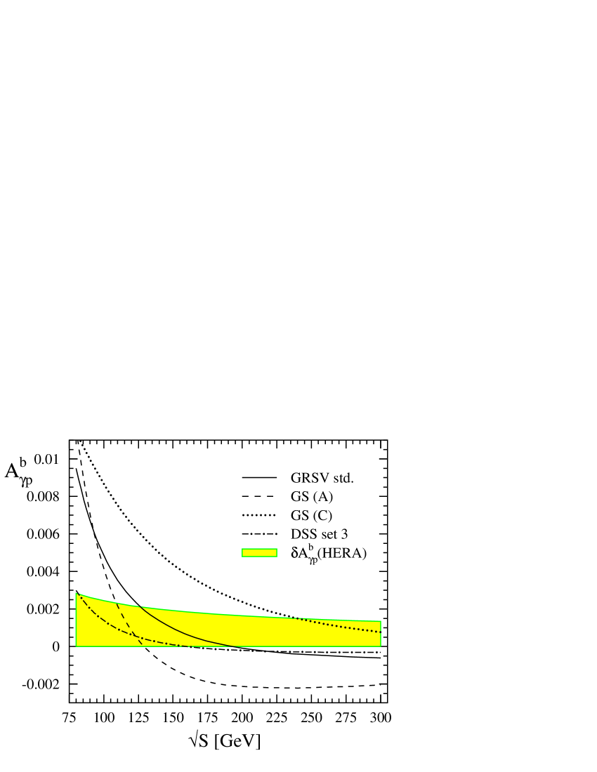
Figure 9: The longitudinal spin asymmetry $A_{\gamma p}^{b}$ for total bottom photoproduction in NLO in the HERA energy range for $m=4.5\,\mathrm{GeV}$, $\mu_{f}=\mu_{r}=2m$ and four different sets of NLO polarized parton densities [8, 9, 11]. The “error band” is an estimate for the expected statistical accuracy $\delta A_{\gamma p}^{b}$ for such a measurement at a polarized HERA (see text).

In Fig. 9 we turn to the longitudinal spin asymmetry $A_{\gamma p}^{b}$ for total bottom quark photoproduction $(m=4.5\,\mathrm{GeV})$ in NLO for HERA energies for four different sets of polarized parton distributions [8, 9, 11] which mainly differ in $\Delta g$. The results obtained for the different sets of parton densities are well separated and sensitive to the different $\Delta g$, but $A_{\gamma p}^{b}$ is extremely small. Since $A_{\gamma p}^{c}$ already appears to be unmeasurable at HERA, the prospects for a meaningful measurement of $A_{\gamma p}^{b}$ seem to be not very promising at the first sight, since bottom cross sections are smaller due to the larger $b$ quark mass and the smaller heavy quark charge $(e_{b}/e_{c})^{2}=1/4$. However, $b$ quarks are experimentally much easier to detect, e.g., through their longer lifetime (secondary vertex tag), which might compensate these shortcomings. The shaded band in Fig. 9 illustrates the expected statistical accuracy for such a measurement at HERA estimated via

$$\delta A_{\gamma p}^{b}\simeq\frac{1}{P_{e}P_{p}}\frac{1}{\sqrt{\varepsilon_{b}{\cal{L}}\sigma_{\gamma p}^{b}}}$$ (68)

assuming a polarization $P_{e,p}$ of the electron and proton beams of about $70\%$, an integrated luminosity of ${\cal{L}}=500\,\mathrm{pb}^{-1}$ [12], and an optimal detection efficiency of $\varepsilon_{b}=0.05$ [44].

Finally, let us turn to some results for differential distributions. Although their experimental relevance seems to be remote, apart from $p_{T}$ and $y$ acceptance cuts, a comparison of the LO and NLO distributions is of theoretical interest to understand in which kinematical regions the corrections are most relevant.

Figure 10: $x_{T}$ differential polarized anticharm photoproduction cross section $d\Delta\sigma^{c}_{\gamma p}/dx_{T}$ in LO and NLO according to Eqs. (59)-(6) for $\sqrt{S}=10$ and 200 GeV and two sets of polarized parton distributions [8, 11]. The bands with forward (NLO) and backward (LO) slanted hatches correspond to the uncertainty due to independent variations of $\mu_{f}$ and $\mu_{r}$ (see text). LO results are denoted by stars, and the “GRSV std.” curves for $\sqrt{S}=200\,\mathrm{GeV}$ are multiplied by $1/8$.

In Fig. 10 we show the rapidity integrated polarized cross section in LO and NLO as a function of $x_{T}$ according to Eqs. (59)-(6). Two values of $\sqrt{S}$ (10 and 200 GeV) and the GRSV “standard” [8] and DSS “set 3” [11] polarized parton densities are used. For the GRSV results the theoretical uncertainty of varying $\mu_{f}^{2}$ and $\mu_{r}^{2}$ independently in the range $a(p_{T}^{2}+m^{2})$ with $a=1/4,\ldots,4$ is illustrated by the bands with forward (NLO) and backward (LO) slanted hatches. All curves are calculated for the choice $a=1$ and the LO results are marked by stars. The NLO corrections are sizable, but the NLO shape is very similar to the LO one. Note that the large corrections for the GRSV [8] densities are to a large extent due to the differences between the poorly constrained LO and NLO $\Delta g$. We have made a similar observation for the total cross section in [20]; using the GS [9] densities (not shown) this effect would be even more pronounced. The GRSV and DSS curves only differ in size, due to the much smaller DSS “set 3” gluon, but not in shape. As for the total cross section in Fig. 7 it turns out that the scale uncertainties are reduced in NLO. For example, at $x_{T}=0.1$ the NLO result varies by $-20\%$ to $55\%$ whereas the LO result varies by $-35\%$ to $75\%$. For $\sqrt{S}=200\,\mathrm{GeV}$ the scale dependence is similar in NLO, but even worse in LO.

Figure 11: Rapidity $y$ differential polarized anticharm distribution $d\Delta\sigma^{c}_{\gamma p}/dy$ at $\sqrt{S}=10\,\mathrm{GeV}$ in NLO and LO according to Eqs. (59)-(6) and using $\mu_{f}=\mu_{r}=2m$. The light quark induced NLO contribution is shown separately. For comparison the dotted curve displays the NLO unpolarized distribution scaled down by a factor 8.

In Figs. 11 and 12 we show the c.m.s. rapidity $y$ and $x_{F}$ differential polarized anticharm photoproduction cross sections according to Eqs. (59)-(6). Since $p_{T}$ is integrated over the entire kinematical range, we choose $\mu_{f}=\mu_{r}=2m$ as the hard scales here. The distributions are asymmetric in $y$ and $x_{F}$ and the heavy quark is dominantly produced “backward” with respect to the incoming photon, i.e., in the direction of the proton. The NLO results are always larger than the LO ones and deviate in shape. In both figures the unpolarized distributions, scaled down to the size of the polarized one, are shown for comparison. The genuine NLO contribution with light quarks in the initial state is shown separately and appears to be negligible in the entire $y$ and $x_{F}$ range.

Figure 12: As in Fig. 11, but now as a function of $x_{F}$. The NLO unpolarized result is divided by a factor $11$ here.

7 Summary

To conclude, we have presented the details of the first complete NLO QCD calculation of heavy flavor photoproduction with longitudinally polarized beam and target. We have provided all relevant intermediate steps of our calculation, in particular we have given complete analytical results for the soft plus virtual gluon cross section. A compact notation was introduced to present both the unpolarized and polarized results simultaneously, and whenever possible we have compared our results to the existing unpolarized calculations and found complete agreement. Similarly, for the abelian part of our unpolarized and polarized results, which can be compared to Refs. [30] analytically.

As phenomenological applications of our results we have first explored the theoretical uncertainties due to the independent variation of the factorization and renormalization scales and due the unknown precise value of the charm quark mass. It was found that the scale dependence is much reduced in NLO, which clearly demonstrates the usefulness of our NLO results in future determinations of the polarized gluon density $\Delta g$, for instance, by the COMPASS experiment. It was critically discussed that the value of the charm quark mass is one of the major uncertainties in a measurement of $\Delta g$ at fixed target energies. NLO estimates for the total bottom quark spin asymmetry accessible in a possible future polarized collider mode of HERA were presented. Finally, we have presented for the first time $x_{T}$, $y$, and $x_{F}$ spin-dependent differential single anticharm photoproduction cross sections in NLO. Although their experimental relevance seems to be remote, our differential expressions are useful for $p_{T}$ and $y$ acceptance cuts for upcoming “total” cross section measurements, in particular at COMPASS.

Appendix A: Kinematics and Hat Phase Space

The phase space calculation for the $2\to 3$ processes is conveniently performed in the c.m.s. frame of the two outgoing unobserved partons [24, 25, 31] (we follow here as far as possible the notations in App. B of [31]):

$$k_{3} = \left(\omega_{3},k_{3}^{x},\omega_{3}\sin\theta_{1}\cos\theta_{2},\omega_{3}\cos\theta_{1},\hat{k}_{3}\right)\;\;,$$

$$p_{1} = \left(E_{1},p_{1}^{x},-\omega_{3}\sin\theta_{1}\cos\theta_{2},-\omega_{3}\cos\theta_{1},\hat{p}_{1}\right)\;\;.$$ (A1)

Since $k_{3}+p_{1}=0$, only one $(n-4)$-dimensional vector $\hat{k}\equiv\hat{k}_{3}=-\hat{p}_{1}$ remains and similarly $k_{3}^{x}=-p_{1}^{x}$. The $x$-components need not to be specified, since the matrix elements do not depend on them, and hence the $x$-integrations can be trivially performed. The other three observed momenta $k_{1}$, $k_{2}$, and $p_{2}$ can be oriented in such a way that they lie in the $y-z$ plane with vanishing hat components. There are three sets depending on which vector is chosen to point in the $z$ direction. As outlined in Sec. 4, the whole calculation can be performed by using only one of these sets. “Set I” is given by

$$k_{1} = \left(\omega_{1},0,|\vec{p}|\sin\Psi,|\vec{p}|\cos\Psi-\omega_{2},\hat{0}\right)\;\;,$$

$$k_{2} = \left(\omega_{2},0,0,\omega_{2},\hat{0}\right)\;\;,$$ (A2)

$$p_{2} = \left(E_{2},0,|\vec{p}|\sin\Psi,|\vec{p}|\cos\Psi,\hat{0}\right)\;\;,$$

where the kinematical quantities in (Appendix A: Kinematics and Hat Phase Space) and (Appendix A: Kinematics and Hat Phase Space) are determined from on-mass-shell constraints and momentum conservation [31]:

$$\omega_{1}=\frac{s+u_{1}}{2\sqrt{s_{4}+m^{2}}}\;\;,\;\;\omega_{2} = \frac{s+t_{1}}{2\sqrt{s_{4}+m^{2}}}\;\;,\;\;\omega_{3}=\frac{s_{4}}{2\sqrt{s_{4}+m^{2}}}\;\;,$$

$$E_{1}=\frac{s_{4}+2m^{2}}{2\sqrt{s_{4}+m^{2}}}\;\;, \;\;E_{2}=-\frac{t_{1}+u_{1}+2m^{2}}{2\sqrt{s_{4}+m^{2}}}\;\;,$$ (A3)

$$|\vec{p}|=\frac{\sqrt{(t_{1}+u_{1})^{2}-4m^{2}s}}{2\sqrt{s_{4}+m^{2}}}\;\;, \;\;\cos\Psi=\frac{t_{1}s_{4}-s(u_{1}+2m^{2})}{(s+t_{1})\sqrt{(t_{1}+u_{1})^{2}-4m^{2}s}}\;\;.$$

In a second parametrization of the momenta (“set II”) $u^{\prime}$ and $u_{7}$ in (21) are of the [ab]-type instead of $t^{\prime}$ and $u_{6}$ in set I. The combined use of these two sets, depending on which type of Mandelstam variables in the denominator has to be integrated, is sufficient to avoid any appearance of auxiliary quantities like $u_{6}^{\prime}$ introduced in (26). In set II we have

$$k_{1} = \left(\omega_{1},0,0,\omega_{1},\hat{0}\right)\;\;,$$

$$k_{2} = \left(\omega_{2},0,|\vec{p}|\sin\Psi,|\vec{p}|\cos\Psi-\omega_{1},\hat{0}\right)\;\;,$$ (A4)

$$p_{2} = \left(E_{2},0,|\vec{p}|\sin\Psi,|\vec{p}|\cos\Psi,\hat{0}\right)\;\;,$$

with the same relations as in (Appendix A: Kinematics and Hat Phase Space) except for

$$\cos\Psi=\frac{u_{1}s_{4}-s(t_{1}+2m^{2})}{(s+u_{1})\sqrt{(t_{1}+u_{1})^{2}-4m^{2}s}}\;\;.$$ (A5)

The derivation of the two-to-three body phase space formula ${\mathrm{dPS}_{3}}$ is standard, and we concentrate here only on the new aspects due to the the additional $(n-4)$-dimensional hat-space integration in the polarized case. The calculation of ${\mathrm{dPS}_{3}}$ is facilitated by introducing a pseudoparticle with momentum $p=p_{1}+k_{3}$, i.e., the sum of the momenta of the two unobserved partons. ${\mathrm{dPS}_{3}}$ can then be separated into a $2\to 2$ and a $1\to 2$ phase space. Only the latter “decay” of the pseudoparticle into unresolved partons depends on the hat-space with the choice of coordinates explained above. This non-trivial integration is then given by

$$1\rightarrow 2=\int d^{n}k_{3}\,d^{n}p_{1}\delta^{+}(k_{3}^{2})\delta^{+}(p_{1}^{2}-m^{2})\delta^{(n)}(p-k_{3}-p_{1})\;\;.$$ (A6)

Using (Appendix A: Kinematics and Hat Phase Space) and (Appendix A: Kinematics and Hat Phase Space), i.e., $p=(\sqrt{s_{4}+m^{2}},0,0,0,\hat{0})$, and the fact that the matrix elements depend only on $\hat{k}^{2}$, we can evaluate (A6) easily by integrating $k_{3}$, $p_{1}^{x}$ and the angles of $\hat{k}$

$$1\rightarrow 2 = \frac{\pi^{n/2-2}}{\Gamma(n/2-2)}\frac{s_{4}^{2}}{8(s_{4}+m^{2})^{3/2}}\int_{0}^{\pi}\int_{0}^{\pi}d\theta_{1}d\theta_{2}\sin^{2}\theta_{1}\sin\theta_{2}$$ (A7)

$$\cdot\int_{0}^{\hat{k}_{max}^{2}}{d}\hat{k}^{2}(\hat{k}^{2})^{n/2-3}\left[{\frac{s_{4}^{2}}{4(s_{4}+m^{2})}\sin^{2}\theta_{1}\sin^{2}\theta_{2}-\hat{k}^{2}}\right]^{-\frac{1}{2}}$$

$$= \frac{\pi^{n/2-2}}{\Gamma(n/2-2)}\frac{s_{4}^{n-3}}{[4(s_{4}+m^{2})]^{n/2-1}}\int_{0}^{\pi}\int_{0}^{\pi}d\theta_{1}d\theta_{2}\sin^{n-3}\theta_{1}\sin^{n-4}\theta_{2}\int_{0}^{1}dx\frac{x^{n/2-3}}{\sqrt{1-x}}$$

$$= \frac{\pi^{n/2-2}}{4}\frac{\Gamma(n/2-1)}{\Gamma(n-3)}\frac{s_{4}^{n-3}}{(s_{4}+m^{2})^{n/2-1}}\int d\Omega_{n-4}\;{\cal{I}}\;\;,$$

with the following abbreviations for the remaining integrations

$$\int d\Omega_{n-4} \equiv \int_{0}^{\pi}\int_{0}^{\pi}d\theta_{1}d\theta_{2}\sin^{n-3}\theta_{1}\sin^{n-4}\theta_{2}\;\;,$$ (A8)

$${\cal{I}} \equiv \frac{1}{B(1/2,n/2-2)}\int_{0}^{1}dx\frac{x^{n/2-3}}{\sqrt{1-x}}\;\;.$$ (A9)

Furthermore we have used the definition

$$x\equiv\hat{k}^{2}/\hat{k}_{max}^{2}=\frac{4(s_{4}+m^{2})\hat{k}^{2}}{s_{4}^{2}\sin^{2}\theta_{1}\sin^{2}\theta_{2}}\;\;.$$ (A10)

Comparing (A7) with (B10) in Ref. [31], we see that the dependence on the hat momenta has been completely absorbed into the additional integral ${\cal{I}}$. Thus we can schematically write for the full $2\to 3$ phase space formula

$${\mathrm{d}PS}_{3}(\theta_{1},\theta_{2})={\mathrm{d}PS}_{3,{\mathrm{u}np}}(\theta_{1},\theta_{2})\times{\cal{I}}\;\;,$$ (A11)

where (one should keep in mind that (B14) in [31] already includes the flux factor, etc.)

$${\mathrm{d}PS}_{3}(\theta_{1},\theta_{2})=dt_{1}du_{1}\,\frac{1}{s}\frac{(4\pi)^{-n}}{\Gamma(n-3)}\left(\frac{t_{1}u_{1}-m^{2}s}{s}\right)^{\frac{n}{2}-1}\frac{s_{4}^{n-3}}{(s_{4}+m^{2})^{n/2-1}}\int d\Omega_{n-4}\;\;.$$ (A12)

Notice that (A7)-(A12) agree in the limit $m^{2}\to 0$ with the result presented in [26].

The vast majority of terms in the matrix elements do not depend on $\hat{k}^{2}$ and the rest is proportional to $\hat{k}^{2}$, so that one finds only two cases ($n=4+\varepsilon$):

$${\cal{I}}\cdot 1 \Rightarrow {\mathrm{d}PS}_{3}(\theta_{1},\theta_{2})={\mathrm{d}PS}_{3,{\mathrm{u}np}}(\theta_{1},\theta_{2})\;\;,$$

$${\cal{I}}\cdot\hat{k}^{2} \Rightarrow {\mathrm{d}PS}_{3}(\theta_{1},\theta_{2})={\mathrm{d}PS}_{3,{\mathrm{u}np}}(\theta_{1},\theta_{2})\;\varepsilon\;\frac{s_{4}^{2}\sin^{2}\theta_{1}\sin^{2}\theta_{2}}{4(s_{4}+m^{2})}\;\;.$$ (A13)

The IR poles in our calculation stem from terms diverging as $1/s_{4}^{2}$ for $s_{4}\rightarrow 0$. Such poles are canceled by the factor $s_{4}^{2}$ in (Appendix A: Kinematics and Hat Phase Space). The M poles in the matrix elements have the collinear structure $\sin^{1+\varepsilon}\theta_{1}/(1-\cos\theta_{1})$, and again we find that due to the factor $\sin^{2}\theta_{1}$ in (Appendix A: Kinematics and Hat Phase Space) one gets finite results. Thus all hat integrations turn out to be infrared and collinear safe. Due to the extra $\varepsilon$ in (Appendix A: Kinematics and Hat Phase Space) all hat contributions are then of ${\cal O}(\varepsilon)$ and drop out when the $\varepsilon\rightarrow 0$ limit is taken in the end. Note that the heavy quark mass plays the role of an infrared regulator here. Collecting the $s_{4}\/$-factors in (Appendix A: Kinematics and Hat Phase Space) and (23) one gets $s_{4}^{3+\varepsilon}/(s4+m^{2})^{2+\varepsilon/2}$. For $m\rightarrow 0$ one then has $s_{4}^{1+\varepsilon/2}$, which is not sufficient to cancel the $1/s_{4}^{2}$ contributions. Thus in the massless case one picks up extra finite contributions from the hat-space integration with infrared poles [26], whereas collinear safety still holds.

Appendix B: Tensor Integrals - Some Remarks

When performing the Passarino-Veltman decomposition [32] various scalar integrals appear which at a first glance are not listed in [31]. However, they can always be cast in the form of [31]. For example, shifting the loop momentum $q\rightarrow q+p_{2}$ immediately yields

$$C_{0}(p_{1},-k_{1}-k_{2},0,m,m)=C_{0}(p_{2},p_{1},m,0,m)\;\;.$$ (B1)

In less simple cases one can easily find the necessary relations by inspecting the Feynman parametrization of the integral. For the three point functions $C_{0}(q_{1},q_{2},m_{1},m_{2},m_{3})$ the Feynman parameter integral has a denominator $[q^{2}-{\cal C}]^{3}$ with ${\cal C}=-abq_{1}^{2}-ac(q_{1}+q_{2})^{2}-bcq_{2}^{2}+am_{1}^{2}+bm_{2}^{2}+cm_{3}^{2}$, where $a,~{}b,~{}c$ are functions of the two Feynman parameters with $a+b+c=1$. We can then prove, for instance,

$$C_{0}(p_{1}-k_{1},-k_{2},0,m,m)=C_{0}(p_{1},-k_{1},0,m,m)\;\;.$$ (B2)

by simply inserting the momenta and masses in ${\cal C}$ and interchanging $b\leftrightarrow c$. It should be noted that exploiting the freedom to re-assign the parameters is also essential for explicitly calculating the set of basic scalar integrals.

When decomposing the tensorial four point functions for the box graphs in Figs. 3 (a) and (b), one has to keep the rather lengthy intermediate expressions as short as possible. For the calculation of the QED-like box [30], Fig. 3 (a), one can show that eight of the twenty-three scalar coefficients $D_{ij}$ are not independent:

$$D_{11}=D_{12}+D_{13}\;\;,\qquad D_{24}=(D_{21}+D_{22}-D_{23})/2\;\;,$$

$$D_{25}=(D_{21}-D_{22}+D_{23})/2\;\;,\qquad D_{31}=-2D_{32}-2D_{33}+3D_{36}+3D_{37}\;\;,$$

$$D_{34}=-D_{32}-D_{33}+2D_{36}+D_{37}\;\;,\qquad D_{35}=-D_{32}-D_{33}+D_{36}+2D_{37}\;\;,$$ (B3)

$$D_{310}=(-D_{32}-D_{33}+D_{36}+D_{37}+D_{38}+D_{39})/2\;\;,\qquad D_{311}=D_{312}+D_{313}\;\;.$$

To prove this, one starts by replacing $q\to-q$ in (4) and with $-q_{4}=q_{1}+q_{2}+q_{3}$ finds

$$D_{0}(q_{1},q_{2},q_{3},m_{1},m_{2},m_{3},m_{4})=D_{0}(q_{4},q_{3},q_{2},m_{1},m_{4},m_{3},m_{2})\;\;.$$ (B4)

We will abbreviate this result as $D_{0}=\bar{D}_{0}$. Each additional power of the loop momentum in the numerator introduces an extra factor $(-1)$, so that

$$D^{\alpha}=-\bar{D}^{\alpha}\;\;,\qquad D^{\alpha\beta}=\bar{D}^{\alpha\beta}\;\;,\qquad D^{\alpha\beta\gamma}=-\bar{D}^{\alpha\beta\gamma}.$$ (B5)

By writing down for example the vector decomposition and comparing the coefficients, one obtains

$$D_{11}=\bar{D}_{11}\;\;,\qquad D_{12}=\bar{D}_{11}-\bar{D}_{13}\;\;,\qquad D_{13}=\bar{D}_{11}-\bar{D}_{12}\;\;.$$ (B6)

In the case of the QED-like box one encounters $D_{ij}=D_{ij}(p_{1},-k_{1},-k_{2},0,m,m,m)$ and $\bar{D}_{ij}=D_{ij}(p_{2},-k_{2},-k_{1},0,m,m,m)$. But the QED-like box is symmetric with respect to $k_{1}\leftrightarrow k_{2}$ and $p_{1}\leftrightarrow p_{2}$. Thus $D_{ij}=\bar{D}_{ij}$ and one obtains the first relation of (Appendix B: Tensor Integrals - Some Remarks) from (B6) and, analogously, the other relations are derived. For the non-abelian box in Fig. 3 (b) on the other hand, one has $D_{ij}=D_{ij}(-k_{1},p_{1},-k_{2},0,0,m,m)$ and $\bar{D}_{ij}=D_{ij}(p_{2},-k_{2},p_{1},0,m,m,0)$ and furthermore the $k_{1}\leftrightarrow k_{2}$ symmetry is lost as discussed at the end of Sec. 4. Thus here one finds no simple relations between the $D_{ij}$ and the $\bar{D}_{ij}$ that could be exploited to reduce the number of coefficients. One can, of course, check these general arguments explicitly, e.g., for arbitrary momenta and masses one finds $D_{12}-\bar{D}_{12}=D_{13}-\bar{D}_{13}$, see (B6). But this difference only vanishes in the QED case, whereas in the non-abelian case a rest remains that is partly $t_{1}\leftrightarrow u_{1}$ antisymmetric and has $1/\varepsilon^{2}$ and $1/\varepsilon$ poles.

Finally, we note that the gluon self-energy loops in Fig. 3 (i) are zero for massless particles (gluons and light quarks) due to Eq. (5). For the massive quark loop one has to calculate two-point functions of the type $B(k_{2},m,m)$ with $k_{2}^{2}=0$ and $m\neq 0$. Here problems occur when naively applying the decomposition procedure, since one would divide by $k_{2}^{2}$ for the coefficients $B_{1}$ and $B_{21}$. This is the simplest example of the general problem that the standard decomposition breaks down whenever projective momenta do not exist [32]. Of course, the self-energy integral is simple enough to be calculated directly and is given by

$$\!\!\!\!\!\!\!\Pi^{\mu\rho}(k_{2}^{2}=0,m\neq 0)\! = \!ig_{s}^{2}\frac{1}{2}\delta_{ab}\mu^{-\varepsilon}\int\frac{d^{n}q}{(2\pi)^{n}}\frac{{\mathrm{T}r}\left[\gamma^{\mu}(\not\!q+m)\gamma^{\rho}(\not\!q+\not\!k_{2}+m)\right]}{(q^{2}-m^{2})[(q+k_{2})^{2}-m^{2}]}$$ (B7)

$$= \!-\frac{g_{s}^{2}}{4\pi}\delta_{ab}(k_{2}^{\mu}k_{2}^{\rho}-k_{2}^{2}g^{\mu\rho})\frac{1}{6}\left[\frac{2}{\varepsilon}+\gamma_{E}-\ln(4\pi)-\ln\left(\frac{\mu^{2}}{m^{2}}\right)\right]\;\;.$$

Appendix C: Virtual plus Soft Coefficients

We list here the polarized coefficients for the virtual plus soft gluon cross section as defined in Eq. (42):

$$\Delta L_{QED}=\left[-t_{1}(2t_{1}+u_{1})/(tu_{1})-u_{1}(t_{1}+2u_{1})/(t_{1}u)\right]/4+\left[-4m^{2}s(2t_{1}^{2}-t_{1}u_{1}+2u_{1}^{2})\right.$$ (C1)

$${}+\left.t_{1}u_{1}(5t_{1}^{2}+2t_{1}u_{1}+5u_{1}^{2})\right]/(4t_{1}^{2}u_{1}^{2})+\left\{\beta(2m^{2}s+t_{1}^{2}+4t_{1}u_{1}+u_{1}^{2})/(4t_{1}u_{1})\right.$$

$${}+\left.\left[t_{1}^{2}u_{1}^{2}(3t_{1}^{2}+4t_{1}u_{1}+3u_{1}^{2})+4m^{4}(t_{1}^{4}+2t_{1}^{3}u_{1}-8t_{1}^{2}u_{1}^{2}+2t_{1}u_{1}^{3}+u_{1}^{4})\right]/(4t_{1}^{3}u_{1}^{3})\right\}\zeta(2)$$

$${}-\left\{\beta(2m^{2}s+t_{1}^{2}+4t_{1}u_{1}+u_{1}^{2})/8+(-24m^{4}+3t_{1}^{2}+4t_{1}u_{1}+3u_{1}^{2})/8\right\}/(t_{1}u_{1})\ln^{2}\varkappa$$

$${}+\bigg{\{}-\left[2m^{2}t_{1}^{2}(6m^{4}+9m^{2}t_{1}+4t_{1}^{2})+t_{1}(2m^{2}+t_{1})(8m^{4}+9m^{2}t_{1}+2t_{1}^{2})u_{1}\right.$$

$${}+\left.3t(2m^{2}+t_{1})^{2}u_{1}^{2}\right]/(4t^{2}t_{1}^{2}u_{1})-\left[st_{1}^{2}u_{1}(t_{1}+2u_{1})+4m^{4}(t_{1}^{3}+3t_{1}^{2}u_{1}-t_{1}u_{1}^{2}-u_{1}^{3})\right.$$

$${}+\left.2m^{2}(t_{1}^{4}+t_{1}^{3}u_{1}-3t_{1}^{2}u_{1}^{2}-2t_{1}u_{1}^{3}-u_{1}^{4})\right]/(2\beta st_{1}^{2}u_{1}^{2})\ln\varkappa\bigg{\}}\ln\left(\frac{-t_{1}}{m^{2}}\right)$$

$${}+\bigg{\{}-\left[t_{1}u_{1}^{3}(3t_{1}+2u_{1})+4m^{6}(3t_{1}^{2}+4t_{1}u_{1}+3u_{1}^{2})+m^{2}u_{1}^{2}(15t_{1}^{2}+13t_{1}u_{1}+8u_{1}^{2})\right.$$

$${}+\left.2m^{4}u_{1}(12t_{1}^{2}+13t_{1}u_{1}+9u_{1}^{2})\right]/(4t_{1}u^{2}u_{1}^{2})-\left[st_{1}u_{1}^{2}(2t_{1}+u_{1})-4m^{4}(t_{1}^{3}+t_{1}^{2}u_{1}\right.$$

$${}-\left.3t_{1}u_{1}^{2}-u_{1}^{3})-2m^{2}(t_{1}^{4}+2t_{1}^{3}u_{1}+3t_{1}^{2}u_{1}^{2}-t_{1}u_{1}^{3}-u_{1}^{4})\right]/(2\beta st_{1}^{2}u_{1}^{2})\ln\varkappa\bigg{\}}\ln\left(\frac{-u_{1}}{m^{2}}\right)$$

$${}+\left\{(m^{2}s-t_{1}u_{1})/(\beta t_{1}u_{1})+\beta(2m^{2}s+t_{1}^{2}+4t_{1}u_{1}+u_{1}^{2})/(2t_{1}u_{1})\ln(1+\varkappa)\right\}\ln\varkappa$$

$${}+\left\{2m^{2}t_{1}^{2}(u_{1}-t_{1})+t_{1}^{2}(2t_{1}^{2}+2t_{1}u_{1}+u_{1}^{2})-2m^{4}(5t_{1}^{2}+2t_{1}u_{1}+u_{1}^{2})\right\}/(2t_{1}^{3}u_{1})$$

$${}\times{\mathrm{L}i}_{2}\left(\frac{t}{m^{2}}\right)+\left\{2m^{2}(t_{1}-u_{1})u_{1}^{2}+u_{1}^{2}(t_{1}^{2}+2t_{1}u_{1}+2u_{1}^{2})-2m^{4}(t_{1}^{2}+2t_{1}u_{1}+5u_{1}^{2})\right\}$$

$${}/(2t_{1}u_{1}^{3}){\mathrm{L}i}_{2}\left(\frac{u}{m^{2}}\right)+\beta(2m^{2}s+t_{1}^{2}+4t_{1}u_{1}+u_{1}^{2})/(2t_{1}u_{1}){\mathrm{L}i}_{2}(-\varkappa)+\Delta B_{QED}$$

$${}\times\Bigg{\{}1+\frac{s-2m^{2}}{\beta s}\Bigg{(}2\zeta(2)+\Bigg{[}-1+\ln\left(\frac{-t_{1}}{m^{2}}\right)+\ln\left(\frac{-u_{1}}{m^{2}}\right)+4\ln(1-\varkappa)$$

$${}-\ln\varkappa\Bigg{]}\ln\varkappa+4{\mathrm{L}i}_{2}(\varkappa)\Bigg{)}\Bigg{\}}/2\;\;,$$

$$\Delta L_{QED}^{\Delta}=-\Delta B_{QED}\left\{1+\frac{s-2m^{2}}{\beta s}\ln\varkappa\right\}\ln\left(\frac{\Delta}{m^{2}}\right)\;\;,$$ (C2)

$$\Delta L_{OK}=m^{2}s(t_{1}^{2}+u_{1}^{2})/(2t_{1}^{2}u_{1}^{2})+\bigg{\{}-\beta(2m^{2}s+s^{2}+2t_{1}u_{1})/(4t_{1}u_{1})+\bigg{[}-2t_{1}^{2}u_{1}^{2}(2t_{1}^{2}$$ (C3)

$${}+t_{1}u_{1}+2u_{1}^{2})+m^{2}st_{1}u_{1}(7t_{1}^{2}-8t_{1}u_{1}+7u_{1}^{2})-m^{4}(t_{1}^{4}+2t_{1}^{3}u_{1}-26t_{1}^{2}u_{1}^{2}+2t_{1}u_{1}^{3}$$

$${}+u_{1}^{4})\bigg{]}/(2t_{1}^{3}u_{1}^{3})\bigg{\}}\zeta(2)+(-2m^{2}s+t_{1}^{2}+u_{1}^{2})/(4t_{1}u_{1})\left[\ln^{2}\left(\frac{-t_{1}}{m^{2}}\right)+\ln^{2}\left(\frac{-u_{1}}{m^{2}}\right)\right]$$

$${}-\left\{24m^{4}-3s^{2}+2t_{1}u_{1}-\beta(2m^{2}s+s^{2}+2t_{1}u_{1})\right\}/(8t_{1}u_{1})\ln^{2}\varkappa$$

$${}+\Bigg{\{}(m^{2}s+t_{1}^{2})(-m^{2}s+t_{1}u_{1})/(2tt_{1}^{2}u_{1})+\left[t_{1}u_{1}(t_{1}^{2}+u_{1}^{2})-2m^{2}s(2t_{1}^{2}-t_{1}u_{1}+2u_{1}^{2})\right]$$

$${}/(2t_{1}^{2}u_{1}^{2})\ln\left(\frac{-u_{1}}{m^{2}}\right)-\left\{st_{1}^{2}(s-u_{1})u_{1}+2m^{2}\left[st_{1}^{3}+(s^{2}+2t_{1}^{2})u_{1}^{2}\right]-4m^{4}\left[s^{3}+2t_{1}(s^{2}\right.\right.$$

$${}+\left.\left.t_{1}u_{1})\right]\right\}/(2\beta st_{1}^{2}u_{1}^{2})\ln\varkappa\Bigg{\}}\ln\left(\frac{-t_{1}}{m^{2}}\right)+\Bigg{\{}(-m^{2}s+t_{1}u_{1})(m^{2}s+u_{1}^{2})/(2t_{1}uu_{1}^{2})$$

$${}-\left\{s(s-t_{1})t_{1}u_{1}^{2}-4m^{4}\left[s^{3}+2u_{1}(s^{2}+t_{1}u_{1})\right]+2m^{2}\left[su_{1}^{3}+t_{1}^{2}(s^{2}+2u_{1}^{2})\right]\right\}/(2\beta st_{1}^{2}u_{1}^{2})$$

$${}\times\ln\varkappa\Bigg{\}}\ln\left(\frac{-u_{1}}{m^{2}}\right)+\left\{-(m^{2}s-t_{1}u_{1})/(\beta t_{1}u_{1})-\beta(2m^{2}s+s^{2}+2t_{1}u_{1})/(2t_{1}u_{1})\right.$$

$${}\times\left.\ln(1+\varkappa)\right\}\ln\varkappa+\left\{m^{2}t_{1}^{2}(t_{1}-3u_{1})-t_{1}^{3}(t_{1}+2u_{1})+m^{4}(5t_{1}^{2}+2t_{1}u_{1}+u_{1}^{2})\right\}/(2t_{1}^{3}u_{1})$$

$${}\times{\mathrm{L}i}_{2}\left(\frac{t}{m^{2}}\right)+\left\{m^{2}u_{1}^{2}(-3t_{1}+u_{1})-u_{1}^{3}(2t_{1}+u_{1})+m^{4}(t_{1}^{2}+2t_{1}u_{1}+5u_{1}^{2})\right\}/(2t_{1}u_{1}^{3})$$

$${}\times{\mathrm{L}i}_{2}\left(\frac{u}{m^{2}}\right)-\beta(2m^{2}s+s^{2}+2t_{1}u_{1})/(2t_{1}u_{1}){\mathrm{L}i}_{2}(-\varkappa)+\Delta B_{QED}\Bigg{\{}\Bigg{[}-3\zeta(2)$$

$${}+4\ln\left(\frac{\mu_{f}^{2}}{m^{2}}\right)\ln\left(\frac{-u_{1}}{m^{2}}\right)+\ln^{2}\left(\frac{t_{1}}{u_{1}}\right)-2\ln\left(\frac{t_{1}}{u_{1}}\right)\ln\varkappa-\ln^{2}\varkappa+2{\mathrm{L}i}_{2}\left(1-\frac{t_{1}}{u_{1}\varkappa}\right)$$

$${}-2{\mathrm{L}i}_{2}\left(1-\frac{u_{1}}{t_{1}\varkappa}\right)\Bigg{]}/4-\frac{s-2m^{2}}{\beta s}\Bigg{[}2\zeta(2)+\Bigg{\{}\ln\left(\frac{-t_{1}}{m^{2}}\right)+\ln\left(\frac{-u_{1}}{m^{2}}\right)$$

$${}+4\ln(1-\varkappa)-\ln\varkappa\Bigg{\}}\ln\varkappa+4{\mathrm{L}i}_{2}(\varkappa)\Bigg{]}/2\Bigg{\}}\;\;,$$

$$\Delta L_{OK}^{\Delta}=\Delta B_{QED}\!\left\{\!\ln\left(\frac{\Delta}{m^{2}}\right)-\ln\left(\frac{\mu_{f}^{2}}{m^{2}}\right)+\ln\left(\frac{t_{1}}{u_{1}}\right)+\frac{s-2m^{2}}{\beta s}\ln\varkappa\right\}\!\ln\left(\frac{\Delta}{m^{2}}\right)\;\;,$$ (C4)

$$\Delta L_{RF}=\Delta B_{QED}\ln\left(\frac{\mu_{r}}{\mu_{f}}\right)\;\;,$$ (C5)

with $\Delta B_{QED}$ given in Eq. (13), $\beta=\sqrt{1-4m^{2}/s}$, $\varkappa\equiv(1-\beta)/(1+\beta)$, and $t$ and $u$ as defined in (12).

When integrated, the hard gluon cross section diverges logarithmically $\sim\ln^{k}\Delta/m^{2}$ $(k=1,\,2)$ as the IR cutoff $\Delta\rightarrow 0$. This is by definition canceled by the sum of the $\tilde{L}^{\Delta}$ contributions in the soft gluon cross section. If one is interested to show the contributions from the hard and the soft plus virtual contributions separately (as, e.g., in Fig. 1 of [20]), it is thus advisable to shift the $\tilde{L}^{\Delta}$ terms to the, in this way redefined, hard cross section in order to achieve a numerical stable result independent of $\Delta$. For any numerical calculation of physically relevant hadronic cross sections, it is however more practical to directly add the complete soft plus virtual piece to the hard cross section. In both cases this can be achieved by rewriting the soft plus virtual cross section, expanded in powers of $\ln^{k}\Delta/m^{2}$ ($k=0,\,1,\,2)$, as follows [45]

$$\delta(s_{4})\sum_{k=0}^{2}\alpha_{k}\ln^{k}\frac{\Delta}{m^{2}}\rightarrow\Theta(s_{4}-\Delta)A_{k}\alpha_{k}\left|{}_{s_{4}=0}\right.$$ (C6)

with certain coefficients $\alpha_{k}$. (C6) takes properly care of the different distributions $\delta(s_{4})$ and $\Theta(s_{4}-\Delta)$ multiplying the soft and hard parts, respectively, see Eq. (34). As indicated in (C6), the $\alpha_{k}$ have to be always evaluated using the “elastic” $2\to 2$ kinematics, i.e., $s_{4}=0$, even when added to the $2\to 3$ hard cross section. The coefficients $A_{k}$ are given by

$$A_{0}=\frac{1}{s_{4}^{\mathrm{m}ax}-\Delta},\qquad A_{1}=\frac{\ln(s_{4}^{\mathrm{m}ax}/m^{2})}{s_{4}^{\mathrm{m}ax}-\Delta}-\frac{1}{s_{4}},\qquad A_{2}=\frac{\ln^{2}(s_{4}^{\mathrm{m}ax}/m^{2})}{s_{4}^{\mathrm{m}ax}-\Delta}-\frac{2\ln(s_{4}/m^{2})}{s_{4}}$$ (C7)

as can be easily verified by integrating the l.h.s. of (C6) over $(\int_{\Delta}^{s_{4}^{\mathrm{m}ax}}ds_{4})$, which recovers the $\ln^{k}\Delta/m^{2}$ terms.

References

-
[1]
S. Aid et al., H1 collab., Nucl. Phys. B470
(1996) 3;
C. Adloff et al., H1 collab., Nucl. Phys. B497 (1997) 3;
M. Derrick et al., ZEUS collab., Z. Phys. C69 (1996) 607, C72 (1996) 399. - [2] J. Huston et al., CTEQ collab., hep-ph/9801444.
-
[3]
A.D. Martin, R.G. Roberts, W.J. Stirling, and R.S. Thorne, Eur. J. Phys. C4 (1998) 463;
M. Glück, E. Reya, and A. Vogt, hep-ph/9806404. - [4] W. Vogelsang and A. Vogt, Nucl. Phys. B453 (1995) 334.
- [5] A recent overview of the experimental status can be found, for example, in the proceedings workshop Deep Inelastic Scattering off Polarized Targets: Theory Meets Experiment, Zeuthen, Germany, 1997, ed. by J. Blümlein et al., DESY 97-200.
- [6] R. Mertig and W.L. van Neerven, Z. Phys. C70, (1996) 637.
- [7] W. Vogelsang, Phys. Rev. D54 (1996) 2023 (1996), Nucl. Phys. B475 (1996) 47.
- [8] M. Glück, E. Reya, M. Stratmann, and W. Vogelsang, Phys. Rev. D53 (1996) 4775.
- [9] T. Gehrmann and W.J. Stirling, Phys. Rev. D53 (1996) 6100.
-
[10]
G. Altarelli, R.D. Ball, S. Forte, and G. Ridolfi,
Nucl. Phys. B496 (1997) 337, Acta Phys. Pol. B29 (1998) 1145;
K. Abe et al., E154 collab., Phys. Lett. B405 (1997) 180;
D. Adams et al., SMC, Phys. Rev. D56 (1997) 5330. - [11] D. de Florian, O. Sampayo, and R. Sassot, Phys. Rev. D57 (1998) 5803.
- [12] Proceedings of the workshop Physics with Polarized Protons at HERA, Hamburg and Zeuthen, Germany, 1997, ed. by A. De Roeck and T. Gehrmann, DESY-PROCEEDINGS-1998-01.
- [13] G. Baum et al., COMPASS collab., CERN/SPSLC-96-14, CERN/SPSLC-96-30.
-
[14]
D. Hill et al., RHIC Spin collab., letter of intent
RHIC-SPIN-LOI-1991, updated 1993;
G. Bunce et al., Particle World 3 (1992) 1;
Proceedings of the RSC annual meeting, Marseille, CPT-96/P.3400 (1996);
Proceedings of the workshop on RHIC Spin Physics, Riken-BNL Research Center, April 1998, to appear. - [15] M. Glück and E. Reya, Z. Phys. C39 (1988) 569.
- [16] M. Stratmann and W. Vogelsang, Z. Phys. C74 (1997) 641, Proceedings of the 1995/96 workshop on Future Physics at HERA, Hamburg, Germany, eds. G. Ingelman, A. De Roeck, and R. Klanner, p. 815.
-
[17]
G. Altarelli and W.J. Stirling, Particle World 1
(1989) 40;
M. Glück, E. Reya, and W. Vogelsang, Nucl. Phys. B351 (1991) 579;
S.I. Alekhin, V.I. Borodulin, and S.F. Sultanov, Int. J. Mod. Phys. A8 (1993) 1603;
S. Keller and J.F. Owens, Phys. Rev. D49 (1994) 1199;
S. Frixione and G. Ridolfi, Phys. Lett. B383 (1996) 227. - [18] J. Smith and W.L. van Neerven, Nucl. Phys. B374 (1992) 36.
- [19] R.K. Ellis and P. Nason, Nucl. Phys. B312 (1989) 551.
- [20] I. Bojak and M. Stratmann, hep-ph/9804353, to appear in Phys. Lett. B.
- [21] N.S. Craigie, K. Hidaka, M. Jacob, and F.M. Renard, Phys. Rep. 99 (1983) 69.
-
[22]
J. Babcock, D. Sivers and S. Wolfram,
Phys. Rev. D18, 162 (1978);
R.D. Field, Applications of Perturbative QCD, Addison Wesley, 1989;
G. Sterman, An Introduction to Quantum Field Theory, Cambridge University Press, 1993. -
[23]
G. t’Hooft and M. Veltman, Nucl. Phys. B44
(1972) 189;
P. Breitenlohner and D. Maison, Comm. Math. Phys. 52 (1977) 11. - [24] K. Gottfried and J.D. Jackson, Nuovo Cim. 34 (1964) 735.
- [25] R.K. Ellis, M.A. Furman, H.E. Haber, and I. Hinchliffe, Nucl. Phys. B173 (1980) 397.
- [26] L.E. Gordon and W. Vogelsang, Phys. Rev. D48 (1993) 3136.
- [27] M. Jamin and M.E. Lautenbacher, Comput. Phys. Comm. 74 (1993) 265.
- [28] L.M. Jones and H.W. Wyld, Phys. Rev. D17 (1978) 759.
- [29] A.P. Contogouris, S. Papadopoulos, and B. Kamal, Phys. Lett. B246 (1990) 523.
-
[30]
B. Kamal, Z. Merebashvili, and A.P. Contogouris,
Phys. Rev. D51 (1995) 4808, D55 (1997) 3229(E);
G. Jikia and A. Tkabladze, Phys. Rev. D54 (1996) 2030. - [31] W. Beenakker, H. Kuijf, W.L. van Neerven, and J. Smith, Phys. Rev. D40 (1989) 54.
-
[32]
G. Passarino and W. Veltman, Nucl. Phys. B160,
(1979) 151;
W. Beenakker, Ph.D. thesis, Univ. Leiden. - [33] P. Nason, S. Dawson, and R.K. Ellis, Nucl. Phys. B303 (1988) 607, B327 (1989) 49.
-
[34]
J.C. Ward, Phys. Rev. 78 (1950) 1824;
Y. Takahashi, Nuovo Cim. 6 (1957) 371;
J.C. Taylor, Nucl. Phys. B33 (1971) 436;
A.A. Slavnov, Theor. Math. Phys. 10 (1972) 99. - [35] W. Beenakker, private communication.
- [36] A. Devoto and D.W. Duke, Riv. Nuovo Cim. 7 (1984) 1.
- [37] G. Altarelli and G. Parisi, Nucl. Phys. B126 (1977) 298.
-
[38]
J. Kubar-André and F.E. Paige, Phys. Rev.
D19 (1978) 221;
B. Humpert and W.L. van Neerven, Nucl. Phys. B184 (1981) 225. -
[39]
M. Glück and W. Vogelsang, Z. Phys. C55
(1992) 353, C57 (1993) 309;
M. Glück, M. Stratmann, and W. Vogelsang, Phys. Lett. B337 (1994) 373. - [40] M. Glück, E. Reya, and A. Vogt, Phys. Rev. D46 (1992) 1973.
- [41] M. Stratmann and W. Vogelsang, Phys. Lett. B386 (1996) 370.
- [42] M. Glück, E. Reya, and A. Vogt, Phys. Rev. D45 (1992) 3986.
- [43] M. Glück, E. Reya, and A. Vogt, Z. Phys. C67 (1995) 433.
- [44] G. Tsipolitis, private communication.
- [45] W. Beenakker, W.L. van Neerven, R. Meng, G.A. Schuler, and J. Smith, Nucl. Phys. B351 (1991) 507.