The DLLA limit of BFKL in the Dipole Picture

M. B. Gay Ducati ^∗
and
V. P. Gonçalves ^∗∗

Instituto de Física, Univ. Federal do Rio Grande do Sul
Caixa Postal 15051, 91501-970 Porto Alegre, RS, BRAZIL

Abstract: In this work we obtain the DLLA limit of BFKL in the dipole picture and compare it with HERA data. We demonstrate that in leading - logarithmic - approximation, where $\alpha_{s}$ is fixed, a transition between the BFKL dynamics and the DLLA limit can be obtained in the region of $Q^{2}\approx\,150\,GeV^{2}$. We compare this result with the DLLA predictions obtained with $\alpha_{s}$ running. In this case a transition is obtained at low $Q^{2}$ ($\leq 5\,GeV^{2}$). This demonstrates the importance of the next-to-leading order corrections to the BFKL dynamics. Our conclusion is that the $F_{2}$ structure function is not the best observable for the determination of the dynamics, since there is great freedom in the choice of the parameters used in both BFKL and DLLA predictions.

PACS numbers: 12.38.Aw; 12.38.Bx; 13.90.+i;

Key-words: Small $x$ QCD; Perturbative calculations; BFKL pomeron.

1 Introduction

The behaviour of $ep/pp$ scattering in high energy limit and fixed momentum transfer is one of the outstanding open questions in the theory of the strong interactions. In the late 1970s, Lipatov and collaborators [1] established the papers which form the core of our knowledge of Regge limit (high energies limit) of Quantum Chromodynamics (QCD). The physical effect that they describe is often referred to as the QCD pomeron, or BFKL pomeron. The simplest process where the BFKL pomeron applies is the very high energy scattering between two heavy quark-antiquark states, i. e. the onium-onium scattering. For a suficiently heavy onium state, high energy scattering is a perturbative process since the onium radius gives the essential scale at which the running coupling is evaluated. Recently [2, 3, 4] this process was studied in the QCD dipole picture, where the heavy quark-antiquark pair and the soft gluons in the large $N_{c}$ limit are viewed as a collection of color dipoles. In this case, the cross section can be understood as a product of the number of dipoles in one onium state times the number of dipoles in the other onium state times the basic cross section for dipole-dipole scattering due to two-gluon exchange. In [2] Mueller demonstrated that the QCD dipole picture reproduces the BFKL physics. In this work we discuss the BFKL pomeron using the QCD dipole picture.

Experimental studies of the BFKL pomeron are at present carried out mainly in HERA ep collider in deeply inelastic scattering in the region of low values of the Bjorken variable $x\equiv\frac{Q^{2}}{2p.q}$, where $Q^{2}\equiv-q^{2}$. Here $p$ is the four-momentum of the proton and $q$ is the four-momentum transfer of the eletron probe. In this case, QCD pomeron effects are expected to give rise to a power-law growth of the structure functions as $x$ goes to zero. However, this study in deeply inelastic scattering is made difficult by the fact that the low $x$ behaviour is influenced by both short distance and long distance physics [5]. As a result, predictions at photon virtuality $Q$ depend on a nonperturbative input at a scale $Q_{0}<Q$. This makes it difficult to desantangle perturbative BFKL predictions from nonperturbatives effects. Moreover, the program of calculating the next-to-leading corrections to the BFKL equation was only formulated recently [6]. Of course there are uncertainties due to subleading corrections and from the treatment of infrared region of the BFKL equation which will modify the predictions of this approach.

One of the most striking discoveries at HERA is the steep rise of the proton structure function $F_{2}(x,Q^{2})$ with decreasing Bjorken $x$ [7]. The behaviour of structure function at small $x$ is driven by the gluon through the process $g\rightarrow q\overline{q}$. The behaviour of the gluon distribution at small $x$ is itself predicted from perturbative QCD via BFKL equation. This predicts a characteristic $x^{-\lambda}$ singular behaviour in the small $x$ regime, where for fixed $\alpha_{s}$ the BFKL exponent $\lambda=\frac{3\alpha_{s}}{\pi}4ln2$. It is this increase in the gluon distribution with decreasing $x$ that produces the corresponding rise of the structure function. However, the determination of the valid dynamics in the small $x$ region is an open question, since the conventional DGLAP approach [8] can give an excellent description of $F_{2}$ at small $x$. The goal of this letter is to discuss this question.

Recently Navelet et al. [9] applied the QCD dipole model to deep inelastic lepton-nucleon scattering. They assumed that the virtual photon at high $Q^{2}$ can be described by an onium. For the target proton, they made an assumption that it can be approximated by a collection of onia with an average onium radius to be determined from the data. This model described reasonably the $F_{2}$ data in a large range of $Q^{2}(<150\,GeV^{2})$ and $x$.

In this letter we obtain the double-leading-logarithmic-approximation (DLLA) limit of BFKL in the QCD dipole picture using the approach proposed by Navelet et al.. This limit is common to BFKL and DGLAP dynamics. We show that using our DLLA result HERA data can be described in the range $Q^{2}\geq 150\,GeV^{2}$ and all interval of $x$. Moreover, we compare our results with the predictions of Navelet et al. and with the predictions obtained using DGLAP evolution equations in the small-$x$ limit. This letter is organized as follows. In Section 2 the QCD dipole picture is presented. In Section 3 we obtain the proton structure function in this approach and its DLLA limit. In section 4 we apply our result to $F_{2}$ HERA data and present our conclusions.

2 QCD dipole picture

In this section we describe the basic ideas of the QCD dipole picture in the onium-onium scattering. Let ${\cal{A}}$ be the scattering amplitude normalized according to

$$\frac{d\sigma}{dt}=\frac{1}{4\pi}|{\cal{A}}|^{2}\,\,\,.$$ (1)

The scattering amplitude is given by

$${\cal{A}}=-i\int d^{2}x_{1}d^{2}x_{2}\int dz_{1}dz_{2}\Phi^{(0)}(\underline{x}_{1},z_{1})\,\Phi^{(0)}(\underline{x}_{2},z_{2}){\cal{F}}(\underline{x}_{1},\underline{x}_{2})\,\,\,,$$ (2)

where $\Phi^{(0)}(\underline{x}_{i},z_{i})$ is the squared wave function of the quark-antiquark part of the onium wavefunction, $\underline{x}_{i}$ being the transverse size of the quark-antiquark pair and $z_{i}$ the longitudinal momentum fraction of the antiquark. In lowest order ${\cal{F}}$ is the elementary dipole-dipole cross-section $\sigma_{DD}$.

In the large $N_{c}$ limit and in the leading-logarithmic-approximation the radiative corrections are generated by emission of gluons with strongly ordered longitudinal momenta fractions $z_{i}>>z_{i+1}$. The onium wave function with $n$ soft gluons can be calculated using perturbative QCD. In the Coulomb gauge the soft radiation can be viewed as a cascade of colour dipoles emanating from the initial $q\overline{q}$ dipole, since each gluon acts like a quark-antiquark pair. Following [2, 3], we define the dipole density $n(Y,\underline{x},\underline{r})$ such that

$$N(Y,\underline{r})=\int dz_{1}\int d^{2}\underline{x}\,\Phi^{(0)}(\underline{x},z_{1})\,n(Y,\underline{x},\underline{r})$$ (3)

is the number of dipoles of transverse size $\underline{r}$ with the smallest light-cone momentum in the pair greater than or equal to $e^{-Y}p_{+}$, where $p_{+}$ is the light-cone momentum of the onium. The whole dipole cascade can be constructed from a repeated action of a kernel ${\cal{K}}$ on the initial density $n_{o}(\underline{x},\underline{r})$ through the dipole evolution equation

$$n(Y,\underline{x},\underline{r})=n_{o}(\underline{x},\underline{r})+\int_{0}^{Y}dy\int_{0}^{\infty}d\underline{s}\,{\cal{K}}\,(\underline{r},\underline{s})n(y,\underline{x},\underline{s})\,\,\,.$$ (4)

The evolution kernel $\cal{K}$ is calculated in perturbative QCD. For fixed $\alpha_{s}$ and in the limit $N_{c}\rightarrow\infty$ the kernel has the same spectrum as the BFKL kernel. Consequently, the two approaches lead to the same phenomenological results for inclusive observables. The solution of (4) is given by [2, 3]

$$n(Y,\underline{x},\underline{r})=\frac{1}{2}\frac{x}{r}\frac{exp[(\alpha_{P}-1)Y]}{\sqrt{7\alpha C_{F}\zeta(3)Y}}exp\left(-\frac{\pi ln^{2}(x/r)}{28\alpha C_{F}\zeta(3)Y}\right)\,\,\,,$$ (5)

where $\alpha_{P}-1=(8\alpha C_{F}/\pi)ln2$.

The onium-onium scattering amplitude in the leading-logarithmic approximation will be written as in (2), but where $\cal{F}$ is now given by

$${\cal{F}}=\int\frac{d^{2}\underline{r}}{\underline{r}}\frac{d^{2}\underline{s}}{\underline{s}}n(Y/2,\underline{x}_{1},\underline{r})n(Y/2,\underline{x}_{2},\underline{s})\,\sigma_{DD}\,\,.$$ (6)

Consequently, the cross section grows rapidly with the energy because the number of dipoles in the light cone wave function grows rapidly with the energy. This result is valid in the kinematical region where $Y$ is not very large. At large $Y$ the cross section breaks down due to the diffusion to large distances, determined by the last exponential factor in (5), and due to the unitarity constraint. Therefore new corrections should become important and modify the BFKL behaviour [10].

The result (5) was obtained for a process with only one scale, the onium radius. In processes where two scales are present, for example the eletron-proton deep inelastic scattering, this result is affected by non-perturbative contributions [5]. Therefore, the application of BFKL approach at $ep$ scattering must be made with caution.

3 Structure function in the QCD dipole picture

Our goal in this section is to obtain the proton structure functions

$$F_{L,T}(x,Q^{2})=\frac{Q^{2}}{4\pi\alpha_{e.m.}}\,\sigma^{\gamma^{*}\,p}_{L,T}\,\,\,$$ (7)

using the QCD dipole picture. In order to do so we must make the assumption that the proton can be approximately described by onium configurations. Basically, we make use of the assumption

$$\sigma^{\gamma^{*}\,p}_{L,T}=\sigma^{\gamma^{*}\,onium}_{L,T}\times{\cal{P}}\,\,\,,$$ (8)

where ${\cal{P}}$ is the probability of finding an onium in the proton. In order to obtain the $\sigma^{\gamma^{*}\,onium}_{tot}$ we will follow [9], where the $k_{T}$ factorization [11] was used in the context of the QCD dipole model. We have that

$$\sigma^{\gamma^{*}\,onium}_{L,T}=\int d^{2}\underline{r}\,dz\,\Phi^{(0)}(\underline{r},z)\,\sigma^{\gamma^{*}\,dipole}(x,Q^{2},\underline{r})\,\,\,,$$ (9)

where the $\gamma^{*}-dipole$ cross section reads

$$Q^{2}\sigma^{\gamma^{*}\,dipole}(x,Q^{2},\underline{r})=\int d^{2}\underline{k}\int_{0}^{1}\frac{dz}{z}\,\hat{\sigma}_{\gamma^{*}\,g}(\frac{x}{z},\frac{\underline{k}^{2}}{Q^{2}})\,{\cal{G}}(z,\underline{k},\underline{r})\,\,\,.$$ (10)

In (10) $\hat{\sigma}_{\gamma^{*}\,g}$ is the $\gamma^{*}g\rightarrow q\overline{q}$ Born cross section and ${\cal{G}}$ is the non-integrated gluon distribution function. The relation between this function and the dipole density is expressed by

$$\underline{k}^{2}\,{\cal{G}}(z,\underline{k},\underline{r})=\int\frac{\underline{s}^{2}}{\underline{s}}\int_{0}^{1}\frac{dz\prime}{z\prime}n(z\prime,\underline{r},\underline{s})\,\hat{\sigma}_{\gamma^{*}\,d}(\frac{z}{z\prime},\underline{s}^{2}\underline{k}^{2})\,\,\,,$$ (11)

where $n(z\prime,\underline{r},\underline{s})$ is the density of dipoles of transverse size $\underline{s}$ with the smallest light-cone momentum in the pair equal to $z\prime p_{+}$ in a dipole of transverse size $\underline{r}$, of total momentum $p_{+}$. This is given by the solution (5).

After some considerations Navelet et al. obtain

$$Q^{2}\sigma^{\gamma^{*}\,dipole}(x,Q^{2},\underline{r})=4\pi^{2}\alpha_{e.m.}\frac{2\alpha N_{c}}{\pi}\int\frac{d\gamma}{2\pi i}h_{L,T}(\gamma)\frac{v(\gamma)}{\gamma}(\underline{r}^{2}Q^{2})^{\gamma}e^{[\frac{\alpha N_{c}}{\pi}\chi(\gamma)ln\frac{1}{x}]}\,,$$

(12)

where $\frac{\alpha N_{c}}{\pi}\chi(\gamma)$ is the BFKL spectral function (for more details see [9]).

The $\gamma^{*}\,onium$ cross section is obtained using (12) in (9). The result depends on the squared wave function $\Phi^{(0)}$ of the onium state, which cannot be computed perturbatively. Consequently, an assumption must be made. In [9] this dependence is eliminated by averaging over the wave function of transverse size

$$\int dzd^{2}\underline{r}(\underline{r}^{2})^{\gamma}\Phi^{(0)}(\underline{r},z)=(M^{2})^{-\gamma}\,\,\,,$$ (13)

where $M^{2}$ is a scale which is assumed to be perturbative. Therefore the proton structure functions reads

$$F_{L,T}(x,Q^{2})=\frac{2\alpha N_{c}}{\pi}\int\frac{d\gamma}{2\pi i}h_{L,T}(\gamma)\frac{v(\gamma)}{\gamma}(\frac{Q^{2}}{M^{2}})^{\gamma}e^{[\frac{\alpha N_{c}}{\pi}\chi(\gamma)ln\frac{1}{x}]}{\cal{P}}(\gamma,M^{2})\,\,\,,$$ (14)

where ${\cal{P}}(\gamma,M^{2})$ is the Mellin-transformed probability of finding an onium of transverse mass $M^{2}$ in the proton. Using an adequate choice for this probability (see ref. [9]) the proton structure function can be written as

$$F_{L,T}(x,Q^{2})=\frac{2\alpha N_{c}}{\pi}\int\frac{d\gamma}{2\pi i}h_{L,T}(\gamma)\frac{v(\gamma)}{\gamma}(\frac{Q^{2}}{Q_{0}^{2}})^{\gamma}e^{[\frac{\alpha N_{c}}{\pi}\chi(\gamma)ln\frac{1}{x}]}{\cal{P}}(\gamma)\,\,\,.$$ (15)

The expression (15) can be evaluated using the steepest descent method. The saddle point is given by

$$\chi^{\prime}(\gamma_{s})=-\frac{ln\frac{Q^{2}}{Q_{0}^{2}}}{\frac{\alpha N_{c}}{\pi}ln\frac{1}{x}}\,\,.$$ (16)

Using in the expression (16) the expansion of the BFKL kernel near $\gamma=\frac{1}{2}$, we get

$$\gamma_{s}=\frac{1}{2}\left(1-\frac{\frac{Q}{Q_{0}}}{\frac{\alpha N_{c}}{\pi}7\zeta(3)ln\frac{1}{x}}\right)\,\,.$$ (17)

Consequently

$$F_{2}(x,Q^{2}) = F_{T}(x,Q^{2})+F_{L}(x,Q^{2})$$ (18)

$$= C\,a^{\frac{1}{2}}\frac{Q}{Q_{0}}e^{[(\frac{4\alpha N_{c}ln2}{\pi})ln\frac{1}{x}-\frac{a}{2}ln^{2}\frac{Q}{Q_{0}}]}\,\,\,,$$

where

$$a=\left(\frac{1}{\frac{\alpha N_{c}}{\pi}7\zeta(3)ln\frac{1}{x}}\right)\,\,\,.$$ (19)

The parameters $C$, $Q_{0}$ and $\alpha$ are determined by the fit. Using $C=0.077$, $Q_{0}=0.627\,GeV$ and $\alpha\approx 0.11$, Navelet et al. obtained that the expression (18) fits the HERA data [7] in the region $Q^{2}\leq 150\,GeV^{2}$.

In this letter we analize the behaviour of $F_{2}$ obtained by expression (15) in the double leading logarithmic approximation (DLLA). This limit is common to both DGLAP and BFKL dynamics, i.e. it represents the transition region between the dynamics. Therefore, before the determination of the region where the BFKL dynamics (BFKL Pomeron) is valid, we must determine clearly the region where the DLLA limit is valid. In this limit $\chi(\gamma)=\frac{1}{\gamma}$. Using this limit in (16) we get that the saddle point is at

$$\gamma_{s}=\sqrt{\frac{\frac{\alpha N_{c}}{\pi}ln\frac{1}{x}}{ln\frac{Q^{2}}{Q_{0}^{2}}}}\,\,\,.$$ (20)

Consequently, we get

$$F_{2}^{DLLA}(x,Q^{2})=\frac{2\alpha N_{c}}{\pi}\,{\cal{C}}\,\frac{(ln\frac{Q^{2}}{Q_{0}^{2}})^{\frac{1}{4}}}{(\frac{\alpha N_{c}}{\pi}ln\frac{1}{x})^{\frac{3}{4}}}\,e^{\left[2\sqrt{\frac{\alpha N_{c}}{\pi}ln\frac{1}{x}ln\frac{Q^{2}}{Q_{0}^{2}}}\right]}\,\,.$$ (21)

The result (21) reproduces the behaviour of double leading logarithmic approximation. As this result was obtained considering the dipole model, then $\alpha_{s}$ is fixed. The parameters ${\cal{C}}$, $\alpha$ and $Q_{0}$ should be taken from the fit. In the next section we compare this result with HERA data.

4 Results and Conclusions

In this section we compare the expression (21) with the recent H1 data [7]. In order to test the accuracy of the $F_{2}$ parameterization obtained in formula (21), a fit of H1 data has been performed. The parameters obtained were

$${\cal{C}}=0.0035\,,\,\,\,\,Q_{0}=0.45\,\,\mbox{and}\,\,\alpha=0.19\,\,.$$ (22)

In the figures (1) and (2) we present our results at different $Q^{2}$ and $x$. The predictions of Navelet et al. (dashed curve) are also presented. While the expression (18) describes the data in region $Q^{2}\leq 150\,GeV^{2}$, we can see that the expression (21) (solid curve) describes H1 data in kinematical region $Q^{2}\,>\,150\,GeV^{2}$. Therefore the HERA data are described by the DLLA expression in the high $Q^{2}$ region. Moreover, we can conclude that there is a transition between the BFKL behaviour and the DLLA behaviour in the region $Q^{2}\approx 150\,GeV^{2}$. This could be the first evidence of the BFKL behaviour in $F_{2}$. However, this conclusion is not strong since that (18) and (21) were obtained in the leading-logarithmic-approximation, where $\alpha_{s}$ is fixed. Moreover, the parametrizations obtained using the DGLAP evolution equation describes the HERA data [12].

The program of calculating the next-to-leading corrections to the BFKL equation is not still concluded [10]. However, some results may be anticipated. For instance, the NLO BFKL equation must have as limit the DLLA limit in the region where $\alpha_{s}\,log\,\frac{1}{x}\,log\,Q^{2}\,\approx\,1$. This limit is common to both DGLAP and BFKL dynamics. As the NLO corrections to the DGLAP evolution equations are known, the DLLA limit with $\alpha_{s}$ running is well established. The DLLA limit obtained considering the DGLAP evolution equation was largely discussed by Ball and Forte [13]. Consequently we can estimate the importance of $\alpha_{s}$ running in our result. In figure (2) we compare our results with the DLLA predictions with $\alpha_{s}$ running (dot-dashed curve), obtained using DGLAP evolution equations in the small-$x$ limit. In this case the DLLA limit can describe one more large kinematical region. The region $Q^{2}\leq 5\,GeV^{2}$ is not described by DLLA $\alpha_{s}$ running. Consequently, the kinematical region where the BFKL dynamics may be present is restricted to the low $Q^{2}$ region.

Our results are strongly dependent on free parameters, since there is great freedom in the choice of parameters used in both BFKL and DLLA predictions. This comes from theoretical uncertainties, for example, the determination where the pQCD is valid (i.e. the $Q_{0}$ value). However, our qualitative result agrees with the conclusion obtained by Mueller [14], that demonstrated that the BFKL diffusion leads to the breakdown of the OPE at small-$x$. Using the bounds obtained by Mueller we expect that the BFKL evolution can be visible in a limited range of $x$ at $Q^{2}\rightarrow Q_{0}^{2}$. Moreover, our result agrees with the conclusion of Ayala et al. [15], where the shadowing corrections to $F_{2}$ structure function were considered. In this case the anomalous dimension is modified and the BFKL behaviour only can be visible in the region of low $Q^{2}$.

In this paper we calculate the DLLA limit of BFKL in the dipole picture. The determination of this limit is very important, since it is common to BFKL and DGLAP dynamics. Therefore, before the determination of the region where the BFKL dynamics is valid, we must determinate clearly the region where the DLLA limit is valid. We demonstrate that in the leading-logarithmic approximation ($\alpha_{s}$ fixed) a transition region between the BFKL dynamics and the DLLA limit can be obtained in the region of $Q^{2}\approx\,150\,GeV^{2}$. We compare this result with the DLLA predictions obtained with $\alpha_{s}$ running. In this case a transition region is obtained at low $Q^{2}$ ($\leq 5\,GeV^{2}$). This demonstrates the importance of the next-to-leading order corrections to the BFKL dynamics. Our conclusion is that the $F_{2}$ structure function is not the best observable in the determination of the dynamics. From the inclusive measurements of $F_{2}$ it seems improbable to draw any conclusion based on the presently available data. It is theoretically questionable whether it will be possible as long as one considers only one observable. The better observables for determination of the dynamics are the ones associated with processes where only one scale is present, since in these processes it is inambigously possible to isolate the effects of the BFKL behaviour.

Figure Captions

Fig. 1: Behavior of proton structure function predicted by BFKL (18) (dashed curve) and DLLA (21) (solid curve). Data of H1 [7]. See text.

Fig. 2: Behavior of proton structure function predicted by BFKL (18) (dashed curve), DLLA (21) (solid curve) and DLLA with running coupling constant (dot-dashed curve). Data of H1 [7]. See text.

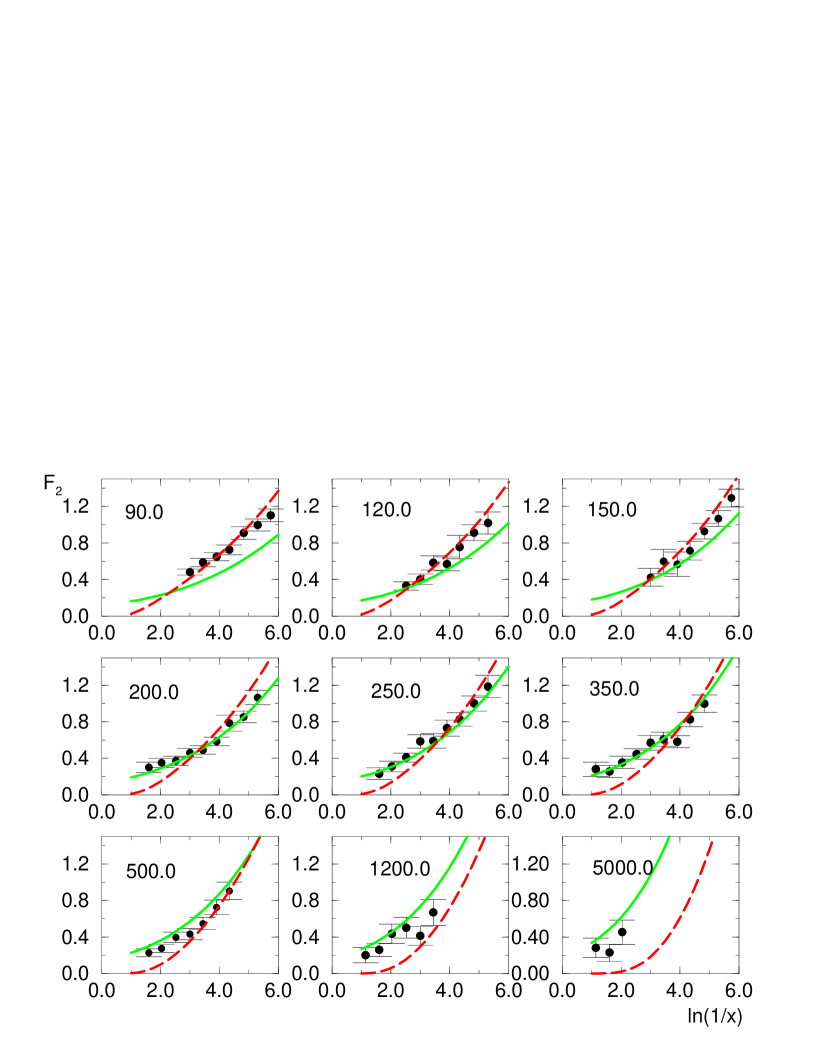
Figure 1:

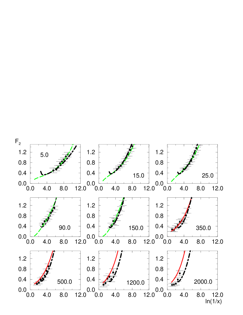
Figure 2:

References

- [1] E.A. Kuraev, L.N. Lipatov and V.S. Fadin. Phys. Lett B60 (1975) 50; Sov. Phys. JETP 44 (1976) 443; Sov. Phys. JETP 45 (1977) 199; Ya. Balitsky and L.N. Lipatov. Sov. J. Nucl. Phys. 28 (1978) 822.
- [2] A. H. Mueller. Nucl. Phys. B415 (1994) 373.
- [3] A. H. Mueller and B. Patel. Nucl. Phys. B425 (1994) 471.
- [4] Z. Chen and A. H. Mueller. Nucl. Phys. B451 (1995) 579.
- [5] J. Bartels, H. Lotter and M. Vogt. Phys. Lett B373 (1996) 215.
- [6] V. S. Fadin and L. N. Lipatov. Nucl. Phys. B477 (1996) 767.
- [7] S. Aid et al.. Nucl. Phys. B470 (1996) 3.
- [8] Yu. L. Dokshitzer. Sov. Phys. JETP 46 (1977) 641; G. Altarelli and G. Parisi. Nucl. Phys. B126 (1977) 298; V. N. Gribov and L.N. Lipatov. Sov. J. Nucl. Phys 28 (1978) 822.
- [9] H. Navelet et al.. Phys. Lett B385 (1996) 357.
- [10] V. S. Fadin aand L. N. Lipatov. hep-ph/9802290.
- [11] S. Catani and F. Hautmann. Nucl. Phys. B427 (1994) 475.
- [12] M. Gluck, E. Reya and A. Vogt. Z. Phys. C67 (1995) 433.
- [13] R. Ball and S. Forte Phys. Lett B335 (1994) 77.
- [14] A. H. Mueller. Phys. Lett B396 (1997) 251.
- [15] A. L. Ayala, M. B. Gay Ducati and E. M. Levin. Nucl. Phys. B493 (1997) 305; Nucl. Phys. B511 (1998) 355.